Detecting Historical Vegetation Changes in the Dunhuang Oasis Protected Area Using Landsat Images

1
College of Earth Environmental Sciences, Lanzhou University, No. 222, Tianshui South Road, Chengguan District, Lanzhou 730000, China
2
School of Civil Engineering, Lanzhou University of Technology, No. 287, Langongping Road, Qilihe District, Lanzhou 730050, China
3
Key Laboratory of Western China’s Environmental systems (Ministry of Education), Lanzhou University, Lanzhou 730000, China
*
Author to whom correspondence should be addressed.
Sustainability 2017, 9(10), 1780; https://doi.org/10.3390/su9101780
Submission received: 25 July 2017
/
Revised: 27 September 2017
/
Accepted: 28 September 2017
/
Published: 30 September 2017
(This article belongs to the Special Issue GISc Contributions to the Study and Understanding of Geographies of Change)
Abstract
:Given its proximity to an artificial oasis, the Donghu Nature Reserve in the Dunhuang Oasis has faced environmental pressure and vegetation disturbances in recent decades. Satellite vegetation indices (VIs) can be used to detect such changes in vegetation if the satellite images are calibrated to surface reflectance (SR) values. The aim of this study was to select a suitable VI based on the Landsat Climate Data Record (CDR) products and the absolute radiation-corrected results of Landsat L1T images to detect the spatio-temporal changes in vegetation for the Donghu Reserve during 1986–2015. The results showed that the VI difference (ΔVI) images effectively reduced the changes in the source images. Compared with the other VIs, the soil-adjusted vegetation index (SAVI) displayed greater robustness to atmospheric effects in the two types of SR images and was more responsive to vegetation changes caused by human factors. From 1986 to 2015, the positive changes in vegetation dominated the overall change trend, with changes in vegetation in the reserve decreasing during 1990–1995, increasing until 2005–2010, and then decreasing again. The vegetation changes were mainly distributed at the edge of the artificial oasis outside the reserve. The detected changes in vegetation in the reserve highlight the increased human pressure on the reserve.
1. Introduction
Dunhuang was an important stop on the ancient Silk Road. Today, it is a famous cultural heritage city. This city is located in Northwestern China in the Western Hexi Corridor in Gansu Province; it lies within the triangle formed by Gansu, Qinghai, and Xinjiang Provinces [1,2,3,4,5,6,7,8,9]. In recent decades, the water-based geological and environmental problems of the Dunhuang basin have worsened, as indicated by the decline of its wetlands and the degradation of its vegetation. The Dunhuang Xihu, Nanhu, Beihu, and Donghu Nature Reserves were established to maintain a natural “green barrier” to protect the ecological diversity and environment of the desert oasis [3,4,10]. The Donghu Nature Reserve is located to the east of Dunhuang and near the artificial oasis; it connects between the Guazhou Oasis and the Dunhuang Oasis (Figure 1) and is of considerable importance to the stability of the two oases.
The increasing environmental pressure on the Donghu Nature Reserve is primarily due to uncontrolled human exploitation of the area and its water resources. In the 1960s and 1970s, the upper reaches of the Shule River and the Dang River were dammed. This intervention caused sections of the rivers to be cut off, reduced the area of wetlands, and caused the decline and die-off of natural vegetation in the reserve [5,6,7,8,9]. In addition, continued increases in the population, the area of the artificial oases [11], and the large-scale planting of cotton, grapes, and other crops that consume large amounts of water in Dunhuang caused a surge in agricultural irrigation. Much of the groundwater has been exploited, leading to a continuing decline in groundwater levels. The problem of water shortages in the nature reserve has become increasingly prominent [3,4]. Protected areas are important for the sustainable economic development of the region [5,8]. The environmental problems of the protected areas in Dunhuang have attracted widespread attention. However, most of the research on the protected areas has focused on the Xihu Reserve [5,6,7,8] and Nanhu Reserve [9], with few studies addressing the Donghu Reserve. Detection of historical changes in the vegetation of the Donghu Nature Reserve over the last 30 years could help the government understand the historical landscape of the reserve. Understanding these changes in vegetation would facilitate identifying the drivers of recent vegetation changes in the Donghu Reserve and provide a reference for research into the vegetation of other reserves.
Vegetation is the primary component of terrestrial ecosystems, and it is a natural medium that connects soil, air, and moisture. It also represents the general status of the environment in a region and acts as an indicator that is used in global change research [12,13]. Vegetation indices (VIs) are important remote sensing (RS) parameters because they reflect the status of vegetation through the digital combination of information from diverse spectrum bands, especially the visible and near-infrared bands. VIs reflect the collective status of chlorophyll, leaf area, coverage, and canopy structure [14,15]. Repeated VI images of the same area can be used to measure variations in the bio-physical characteristics of vegetation, including vegetation coverage. The difference between a later image and an earlier image is called the VI difference (ΔVI) [16]. In a ΔVI image, the unchanged pixels surround the mean value of 0, whereas the changed pixels cluster at the positive and negative ends of the distribution.
Many external factors must be considered when analyzing images of the same area taken at different times; these factors include the soil background, atmospheric conditions, topography, illumination, observation angles, and sensor calibration, all of which can affect the Vis’ values [17,18]. These factors often contribute substantial amounts of noise, which can affect the results of applying the VI values. To accurately evaluate changes in a VI, the images must be calibrated to surface reflectance (SR) data to eliminate or reduce the influence of atmospheric conditions [19,20]. The methods used to invert the true reflectivity of features include both relative and absolute radiation corrections. The FLAASH model is based on the MODTRAN5 radiation transmission model and is commonly used to perform absolute radiation corrections. This model obtains SR values with relatively high accuracy [21]. Landsat’s advanced CDR products provides SR images from the TM sensor [22]. The provisional Landsat 8 Surface Reflectance Code (LaSRC), which employs Moderate Resolution Imaging Spectroradiometer (MODIS) data, is distinctly different from the algorithm used by the USGS to process TM L1T products to obtain SR values [23,24].
The overall goal of the present study was to detect spatio-temporal changes in vegetation in the Donghu Reserve using seven Landsat datasets from different time points (1986, 1990, 1995, 2000, 2005, 2010, 2015). The specific objectives were: (1) explore the impact of the differences between the VIs produced using the CDR products and the results of absolute radiation corrections of the Landsat L1T images on the inferred vegetation changes in the reserve, (2) determine a suitable VI for assessing the vegetation changes within the study area, and (3) analyze the historical changes in the vegetation of the reserve from a spatio-temporal perspective. The present study provides a basis for the study of vegetation changes in other reserves.
2. Study Area and Data
2.1. Study Area
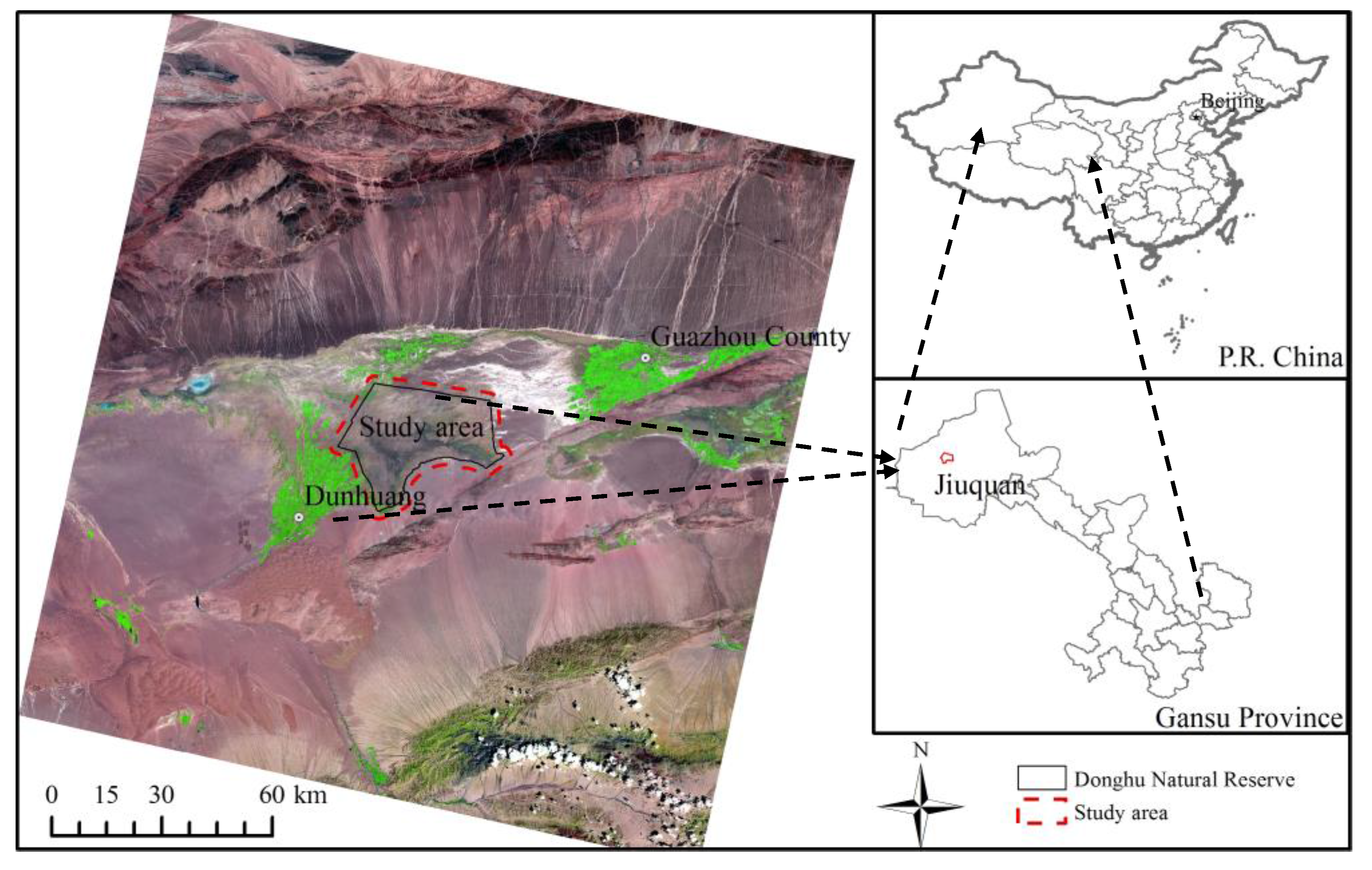
The Donghu Nature Reserve (40°7′51″–40°28′58″ N, 94°47′45″–95°19′41″ E) is located along the Dang River Plain in Dunhuang on the eastern side of an artificial oasis. It covers Yitang Lake, Xindian Lake, and Daquanwan and has an area of approximately 2.7 × 10⁴ km2. The average elevation of the reserve is 1110 m, and the average annual precipitation and evapotranspiration are 39.9 mm and 2490 mm, respectively. The reserve has a warm temperate arid climate. The abundances of water and plants represent barometers of the ecological environment of the desert oasis in Dunhuang, which has been well protected by the local government and relevant departments for many years. However, because of its proximity to the artificial oasis, the reserve has been affected by drought and agricultural production activities. Serious desertification has been observed in the area surrounding the reserve, reeds and other wetland vegetation have declined, and the plant community has experienced serious degradation [25]. In addition, the Yitanghu wetland is rich in nitrate and thick shrubs, and many springs are present in the surrounding area; thus, this area is subject to frequent human activities, such as mining, grazing, digging, and hunting. These activities have exacerbated the degradation of the vegetation in the reserve [26]. The boundaries of the Donghu Reserve were extracted based on the forest resources distribution map of Dunhuang (1:250,000) for 2004. In this study, because the vegetation was the main object of analysis, the mountains in the reserve were masked out, and the area within a 2-km buffer surrounding the reserve (shown by the red line in Figure 1) was the main study area.
2.2. Data
The Landsat images used in this study, which cover the period from 1986 to 2015 and are located at path 137 and row 32, were downloaded from the USGS. The scenes, which were collected by the Landsat 5 TM and Landsat 8 OLI satellites, have a resolution of 30 m and are terrain-corrected Level 1T products and the corresponding Landsat CDR-SR products. As shown in Table 1, the time period covered for each year was July to August [11]. This period corresponds to the best phenological period for the vegetation. The use of a consistent period avoided differences caused by different seasons and allowed for the differentiation of different features in the images.
3. Method
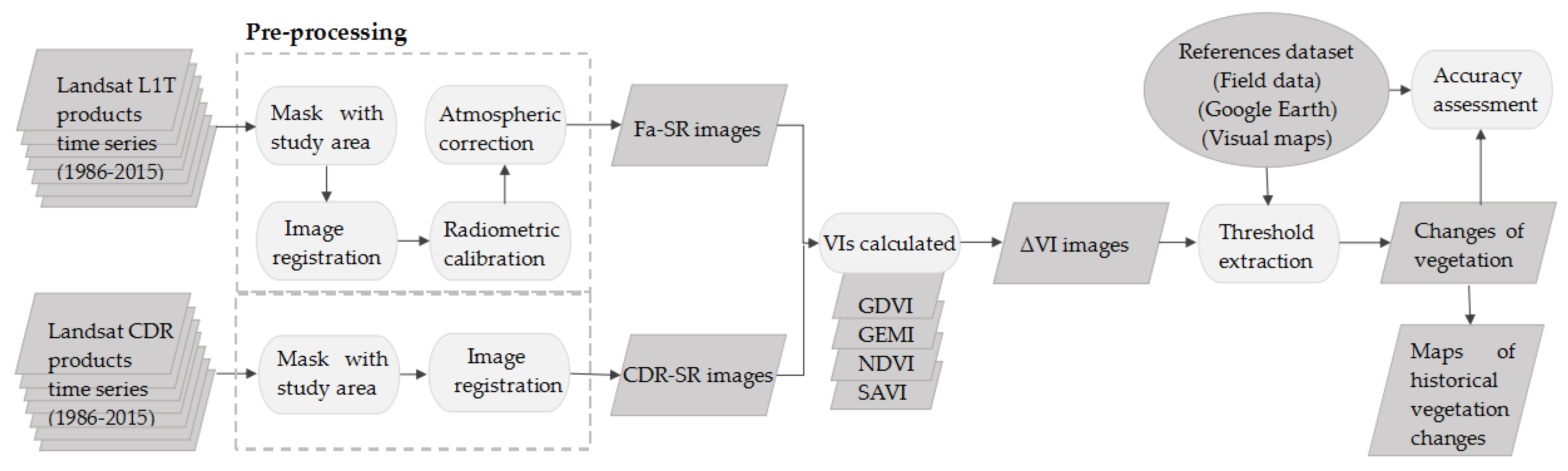
The workflow, shown in Figure 2, primarily includes data preprocessing, evaluation of the FLAASH atmospheric correction, the calculation of the VIs and ΔVIs, the extraction of the vegetation changes based on threshold criteria and the production of maps of the spatio-temporal vegetation changes. These steps are described in detail below.
3.1. Data Preprocessing
To ensure that pairs of images occupying the same position had consistent coordinates, image registration of the different phases was performed when possible to eliminate “pseudo-changes” caused by geometric errors [27]. A Landsat CDR-SR image obtained on 8 August 2015, was selected as the reference image; as required, this image largely reflected clear atmospheric conditions. Although this image did contain cloud-covered areas, the pixels within the study area were not affected [28]. Based on the “Map_Registration_Select GCPs: Image to Image” module in software ENVI v5.1 (Exelis Visual Information Solutions, Boulder, CO, USA), 42 uniformly-distributed points were selected for image registration. To ensure the accuracy of the results, surface pixels that were not prone to warpage and spectral deformation, such as road intersections and inflection points, river confluences, and buildings that did not change over time, were selected as control points. Using the second-order polynomial correction, the registration errors were found to be equal to or less than 0.5 pixels.
The digital number (DN) of each image was transformed into radiance by radiometric calibration. The following conversion formulas were applied to the TM and OLI data, respectively:
where QCAL represents the DN of a pixel; and represent the maximum and minimum DN values of the image, respectively; and and represent the maximum and minimum radiance measured by the sensor, respectively. These values were determined from the metadata of each image.
3.2. FLAASH Atmospheric Correction
FLAASH is an atmospheric correction model that is based on the MODTRAN5 radiation transmission model and produces high-precision results. The atmospheric properties were estimated via feature points on the spectrum of the image pixels using the model instead of using atmospheric data collected at the same time that the images were taken. This process effectively removed scattering by vapor and aerosols. The pixel-based corrections were also able to rectify the effects of cross radiance caused by the proximity between the target pixels and adjacent pixels [29]. In addition, the model performed effective spectral smoothing of the noise caused by artificial suppression, and accurate parameters of the true physical model, such as reflectivity, emissivity, and surface temperature, were obtained. The atmospheric corrections used in the FLAASH model are based on the standard planar Lambertian (or the approximate planar Lambertian) in the range of the solar spectrum in addition to the thermal radiation [21,29]. In this study, seven images with absolute atmospheric corrections were produced using the FLAASH module embedded in ENVI 5.1.
3.3. Vegetation Indices
The following four main VIs were tested to determine the applicability of the CDR-SR and the SR calculated with the FLAASH model (Fa-SR) images: the Normalized Difference Vegetation Index (NDVI), the Generalized Difference Vegetation Index (GDVI), the Global Environment Monitoring Index (GEMI), and the Soil-Adjusted Vegetation Index (SAVI). These VIs employ the spectral information contained in the red () and near-infrared () bands, which facilitates the delineation of vegetation compared with the delineation obtained using other bands. The NDVI and GDVI are ratio indices and derivatives of the Ratio Vegetation Index (RVI) [15]. The SAVI and GEMI use fixed constants instead of the band ratio model. The NDVI is the most widely used VI [30]. The SAVI can reduce the impact of the soil background in areas of sparse vegetation [31], whereas the GDVI has higher sensitivity in areas of sparse vegetation [14]. The GEMI performs well in detecting vegetation in arid areas [32,33].
Since the differences between the CDR-SR images and the Fa-SR images could potentially affect the VI images, a correlation analysis and a linear regression analysis of the VICDR images (which were produced using the CDR-SR images) and the VIFa images (which were produced using the Fa-SR images) were performed to assess the sizes of these differences.
3.4. Detecting Changes in the Vegetation
The VICDR images were ordered in chronological order, and the ΔVICDR images were produced by taking the subsequent image () minus the previous image () in pairs of consecutive images [22]. Here, each ΔVICDR included the four ΔVIs produced from the four Vis’ Equation (3): ΔGDVICDR, ΔGEMICDR, ΔNDVICDR, and ΔSAVICDR. Similarly, each ΔVIFa image included the four ΔVIs produced from the four VIs’ Equation (4): ΔGDVIFa, ΔGEMIFa, ΔNDVIFa, and ΔSAVIFa. A total of 48 ΔVI images were obtained.
Images taken close to the day of the year on which the reference image was taken were selected to reduce the effects of seasonal variation in vegetation. However, the “pseudo-changes” in vegetation caused by differences in the annual data could still be captured by the VI images. The four ΔVI distributions were compared to assess whether such “pseudo-changes” in vegetation caused by changes in the annual data had been captured by the CDR-SR images and whether the Fa-SR images could reduce these effects.
A simple classification extraction was conducted to investigate whether the use of the CDR-SR images, the Fa-SR images and the different VIs (i.e., the NDVI, the GDVI, the GEMI, and the SAVI) affected the mapping of the vegetation changes. Generally, an appropriate threshold was selected to classify the pixels of the ΔVI images as representing a change or no change. Several methods are available to determine these thresholds [34,35,36]. Ideally, independent reference data, such as surface data and high-resolution aerial photographs, would be used to verify the accuracy of the classifications [37]. However, independent reference data were not available for the study area. The upper and lower 5% were selected as the final thresholds based on multiple experiments that combined the field data, Google Earth and visual maps [38]. The upper 5% reflected the positive changes in vegetation, and lower 5% represented the negative changes. The pixels of the 48 ΔVI images were divided into two categories, which reflected either changed or unchanged areas [39]. A 3 × 3 median filter was used to reduce the noise of each of the classified images.
The percentage of consistency between the pixels classified as representing the change using the same threshold in the ΔVICDR images and the corresponding ΔVIFa images was calculated. A high percentage of consistency would indicate that the method of calibrating the SR had little or no effect on the number of pixels that were classified as reflecting changed vegetation. Moreover, the choice of VI can also affect the number of pixels classified as changed; a high consistency shows that the VI has little effect on the different methods of radiometric correction.
3.5. Historical Vegetation Changes
Based on the results of the above analysis, the ΔSAVIFa images were selected to analyze the historical changes in vegetation in the study area. The annual change of vegetation was not spatially invariant over time [22,40]. The changes in vegetation caused by rotation or fallowing of cultivated land or changes in the growth of natural vegetation manifested as steady changes. In the case of wasteland reclamation or serious incursions into previously undisturbed areas, the area of change showed an increasing trend. To investigate these factors, the changed areas (including positive and negative changes) were calculated.
To determine the spatial changes in the study area, six maps derived from the ΔSAVI images reflecting the positive and negative changes were created for all the years to increase the likelihood that all changes in vegetation due to human factors were included.
4. Results
4.1. Comparative Analysis of the VIs
The correlation analysis showed that the four VIs produced using each CDR-SR image displayed a very strong relationship with the corresponding Fa-SR image (R ≥ 0.986). The highest correlation was obtained for the SAVI ( = 0.991, 1995a), followed by the NDVI ( = 0.988, 2010a), the GDVI and the GEMI ( = 0.986, 2010a). The linear regression analysis showed that the largest values of the slope (a) and offset (b) of the four VIs occurred in 1995 compared with the other years. The differences between the pairs of images corresponded to the higher RMSE values in 1995. In general, among the VI images produced from the same CDR-SR images and the Fa-SR images, the lowest values of the RMSE and the strongest correlations were observed for the SAVI images followed by the NDVI images.
4.2. Impact of Vegetation Changes
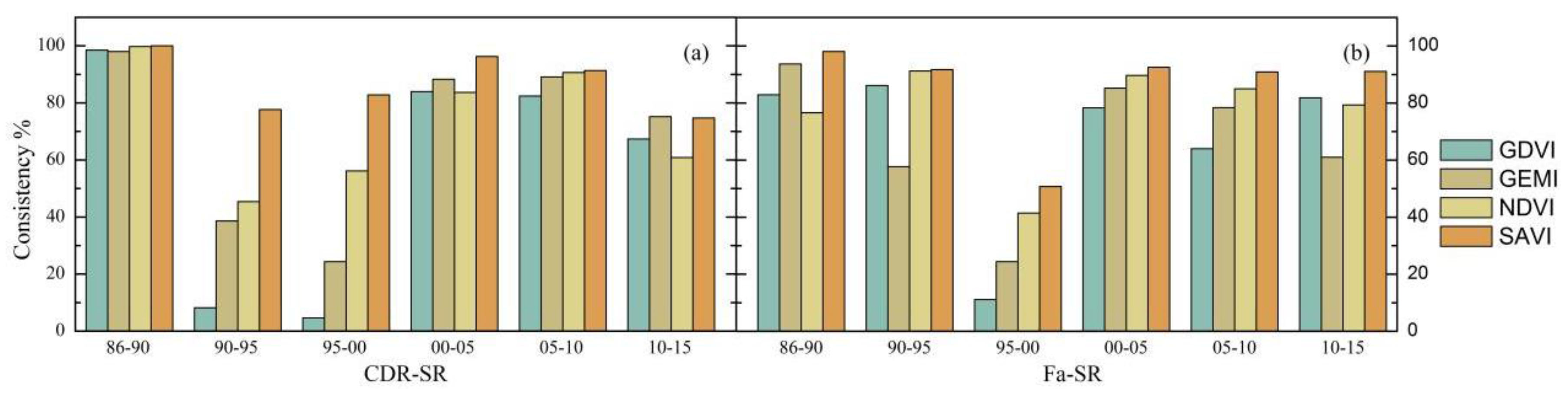
To obtain the actual changes in the surface vegetation rather than spurious effects caused by properties of the images themselves, the areas of vegetation change (including both positive and negative changes) were extracted through a simple classification experiment. The consistency of the classification of the changed vegetation in the ΔVICDR images was the percentage of changed pixels produced by the CDR-SR images, where the changed pixels were extracted using the CDR-SR images and the Fa-SR images (Figure 3a). In addition, the percentage of changed pixels produced using the Fa-SR images, where the changed pixels were extracted by the CDR-SR images and the Fa-SR images, represented the consistency of changed vegetation in the ΔVIFa images (Figure 3b). The consistency between ΔVICDR and ΔVIFa was poor when the same threshold (5%) was used. The worst consistency was obtained in 1995–2000, followed by 1990–1995, which displayed a significant relationship with the larger slope, offset, and RMSE of the VIs calculated using the two kinds of SR images in 1995. The consistency of the two kinds of SR images in the other periods exceeded 60%. However, the changed pixels produced using the CDR-SR images and the Fa-SR images differed among the different VIs and the different periods. The ΔSAVI images displayed a higher consistency than the other ΔVIs between the CDR-SR images and the Fa-SR images (Figure 3).
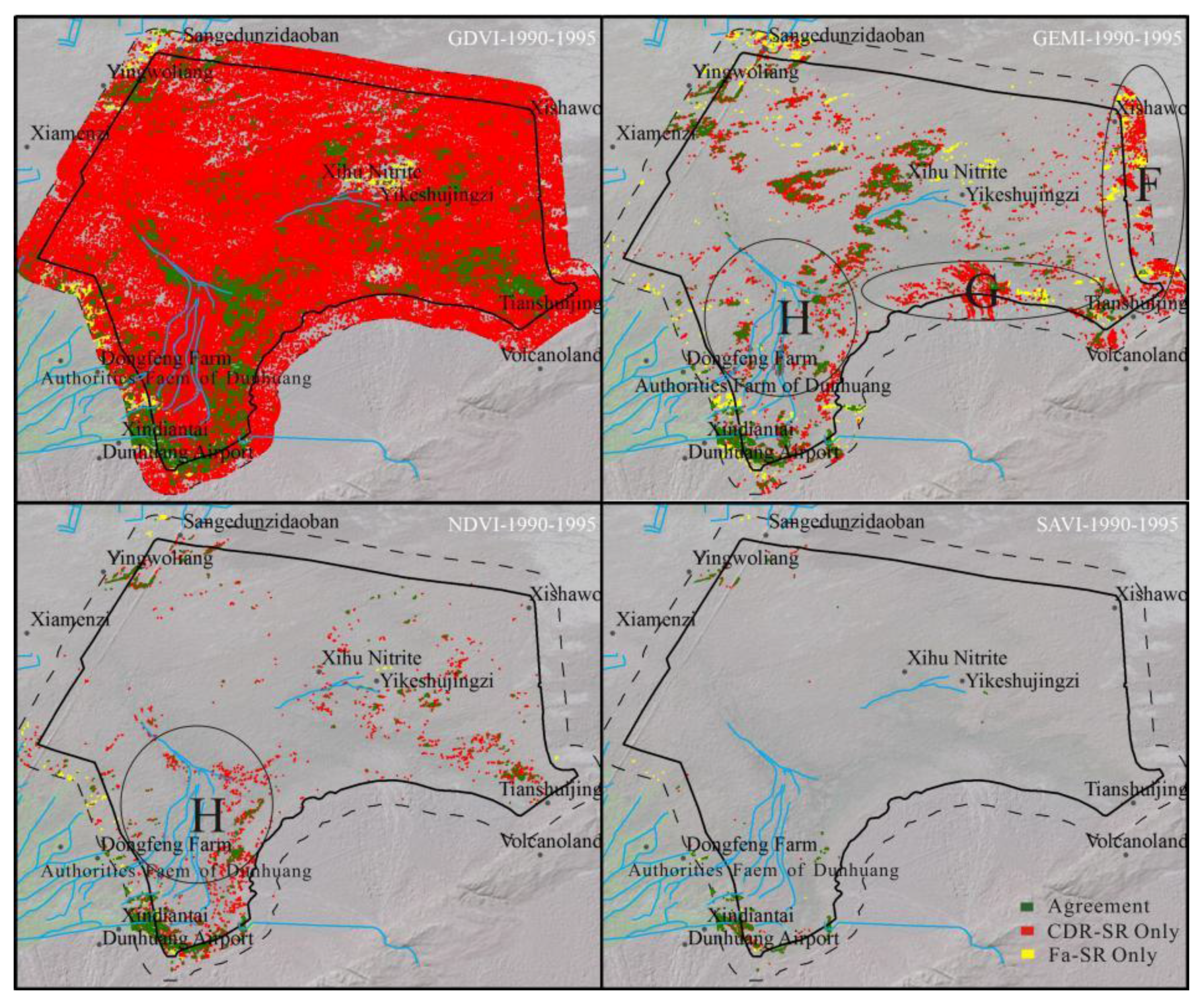
As shown in Figure 3, the worst consistency in the changed pixels contained in the CDR-SR images and Fa-SR images was observed in the periods 1995–2000 and 1990–1995, respectively, and large inconsistencies were observed between the areas of vegetation change obtained using the two types of SR images. Many small changes in the images themselves were captured by the ΔGDVICDR images in 1995–2000 and 1990–1995 (Figure 4 and Figure 5). These changes were monitored for “pseudo-changes” in vegetation. These changes were considered to be disruptive to the extraction of vegetation changes and represented the main reason for the poor consistency. Correspondingly, the ΔVIFa images displayed better performance in eliminating the changes in the images themselves and more accurately reflected the changes in vegetation. Most of the areas of the Gobi landscape (Figure 4: Sections A and B; Figure 5: Section F) and bare rock (Figure 4: Section E; Figure 5: Section G) were monitored for “vegetation changes” in the ΔGEMICDR images. The changes in natural vegetation caused by changes in water were also detected by the ΔNDVICDR and ΔGEMIFa images (Figure 4: Section C and D; Figure 5: Section H). The effect of vegetation changes caused by the soil and image brightness factors were eliminated more completely from the ΔSAVI images than from other ΔVI images. The vegetation changes extracted using the ΔSAVI images mainly reflected vegetation changes (either reductions or increases) in the periphery of the protected area. The corresponding ΔSAVI inconsistent maps displayed similarly spatial patterns of inconsistent as the ΔNDVI images; however, the affected area was significantly reduced.
4.3. Map of Historical Vegetation Changes in the Reserve
The spatial distribution of vegetation changes that occurred from 1986–2015 in the Donghu Reserve are shown in Figure 6. From 1986 to 1990, the most obvious positive changes in vegetation occurred mainly near Xihu nitrate ore and a smaller number of changes (including positive and negative changes) occurred close to Xindiantai, in the southwestern region of the area (Figure 6a). From 1990 to 1995, the vegetation changes occurred mainly at the edges of artificial oases and were primarily distributed near the southwest corner of the Donghu Reserve (Figure 6b). The vegetation changes (including positive and negative changes) gradually appeared in the protected area during 1995–2000, and a large area of positive changes appeared near Yingwoliang, the terminal area of the Shule River (Figure 6c). From 2000 to 2005, there were a large increase in vegetation near Dongfeng Farm and Xindiantai in the southwest corner of the reserve, whereas the vegetation near Yingwoliang showed a marked decrease (Figure 6d). During 2005–2010, the vegetation showed obvious increases around Yingwoliang and Sangedunzidaoban in the northwest corner of the reserve, and the area of changes in vegetation was larger in this period than that in the previous period (Figure 6e). From 2010–2015, vegetation changes simultaneously occurred near Yingwoliang and Xindiantai, in the northwest and southwest corners of the area (Figure 6f).
As showed in Figure 6, obvious changes in the vegetation in the main part of the reserve occurred during 1986–1990; fewer obvious changes occurred in the other periods. These findings indicate that, since 1990, the vegetation in the reserve has generally remained stable. The changed areas were consistently concentrated in the northwest and southwest corners of the reserve, adjacent to the artificial oasis, and were easily affected by human activities. The small plots inside the reserve showed small changes in space and time from 1995–2015.
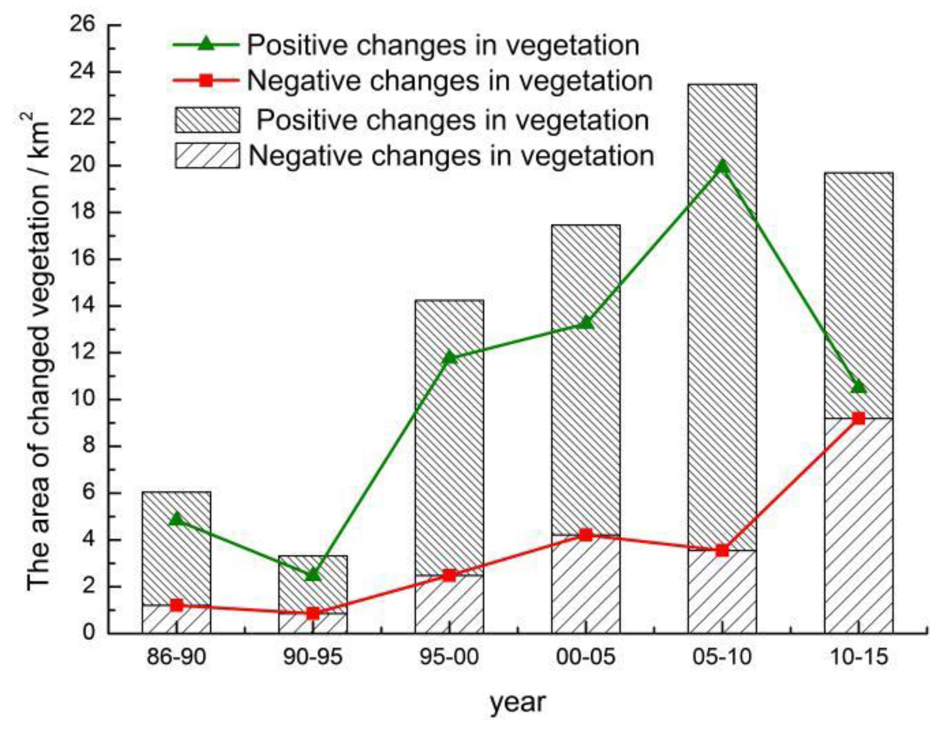
As is shown in Figure 7, the areas reflecting vegetation changes decreased from 1990 to 1995, increased after 1995, and then decreased again until 2010–2015. The positive changes in vegetation showed the same trend as the overall vegetation changes. The area of positive changes was consistently larger than that of negative changes in the period of 1986–2010, whereas the areas of positive and negative changes were similar during 2010–2015. The area of negative changes in vegetation displayed a slight decrease during 1990–1995, increased after 1995, decreased during 2005–2010, and then increased again. However, the positive changes in vegetation dominated the overall trend of changes in vegetation.
5. Discussion
The high correlations between the various VI images calculated using the CDR-SR images and the Fa-SR images occurred because the VIs were calculated using a non-linear combination of the red and near-infrared bands of the SR images. The differences in the offset and slope and the RMSE values were caused by the different radiation transmission models employed in producing the CDR-SR images and the Fa-SR images [22,41]. The linear regression analysis of the VIs showed that the atmospheric correction method used to generate the CDR-SR images and the FLAASH correction method were not equivalent among the VIs.
Obvious differences in the consistency of the vegetation changes produced using ΔVICDR and ΔVIFa with the same threshold were observed, likely because the CDR-SR images and the Fa-SR images used to calculate the VIs were extracted using different radiation transmission equations [22,42]. However, the choice of VIs had a stronger effect on the consistency of the pixels that were classified as changed than the choice of SR images. The ΔGDVI images yielded the worst consistency when the changed vegetation pixels were extracted using the CDR-SR images and the Fa-SR images with the same threshold. Among the ΔVI images, the ΔGDVI images were more sensitive to differences in the images caused by precipitation and different acquisition times; thus, they captured more variable information [14,15]. These phenomena were more pronounced in the CDR-SR images than in the Fa-SR images. The ΔGEMI images eliminated some of the differences associated with the images themselves, although the areas of bare rock and Gobi landscape in the study area were also monitored for vegetation changes. However, the changed pixels extracted using the ΔNDVI and ΔSAVI images were found to have little effect on the residual atmospheric correction effect in the images [31,42]. Subtle changes caused by water and natural vegetation were also detected by the ΔNDVI images, which reduced the ability of the method used here to distinguish the vegetation changes driven by artificial effects from those produced by natural factors. Since the Donghu Reserve is close to the artificial oasis, and beacuse protective forest management has been implemented there, the vegetation changes were mainly caused by human factors [8,9,10]. Thus, the ΔSAVIFa images were used to detect and reflect the changes in vegetation in the Donghu Reserve in this study.
The historical vegetation changes in the Donghu Reserve occurred mainly at the edge of the artificial oasis between 1986 and 2015 (Figure 6). The positive changes in vegetation were consistent with the overall trend in vegetation change (Figure 7). According to Xu et al., Zhang et al. [2,11], and the field investigation, the artificial oasis of the Dang River Plain expanded parallel to the Donghu Reserve. Over the period from 1986 to 1990, the change in the area of the oasis was very small and had little impact on the reserve. The positive changes in vegetation occurred primarily near Xihu nitrate ore, where the vast desert is located, far from the oasis and traffic line and free from human activities; thus, these changes are likely related to natural factors, especially precipitation. The vegetation changes decreased during 1990–1995 because a small increase in the area of the oasis occurred, and the vegetation within the protected area displayed essentially no change during this period. From 1995 to 2010, the artificial oasis near Yingwoliang, Xindiantai, and Dongfeng Farm gradually expanded and encroached on the reserve, resulting in an increase in the area displaying vegetation changes [2]. During 2010–2015, because of the small change in the area of the oasis, the area of vegetation change in the study area decreased [11]. The slight changes in vegetation in the southeast of the reserve were related to the implementation of enclosure management in the region. Since this area is located far from the artificial oasis, the vegetation changes were less strongly controlled by human factors than the areas near the oasis. The vegetation changes in the reserve were mainly related to changes in natural vegetation, and the changes were not obvious.
6. Conclusions
This study showed that the VI images calculated using the CDR-SR images and the Fa-SR images were strongly correlated (R 0.986). The differences in the slope and offset were small, but important. The consistency of the vegetation changes detected using the ΔVICDR and ΔVIFa images was poor during 1990–1995 and 1995–2000. This poor consistency displayed significant relationships with the larger slope, offset, and RMSE of the VIs calculated using the two types of SR images in 1995. However, the consistency of the vegetation changes extracted using the SAVI images was higher than that obtained with the other VIs, and the ΔVIFa images displayed better characteristics in terms of the changes in the images themselves compared with the ΔVICDR images (Figure 3).
The resulting vegetation changes extracted using ΔGDVICDR and ΔGDVIFa included many small changes in the images themselves. Most of the areas of the Gobi landscape and bare rock were monitored for vegetation changes in the ∆GEMICDR images. The changes in natural vegetation caused by changes in water were also detected using the ∆NDVICDR images and the ∆GEMIFa images. Thus, the ΔSAVIFa images were considered to represent the best choice for the extraction of vegetation changes within the study area.
Changes in vegetation have been occurring in the Donghu Reserve since at least 1986. Obvious changes in vegetation in the main part of the reserve were only observed in the period from 1986 to 1990, with fewer changes observed in the other periods. These findings indicate that since 1990, the vegetation in the reserve has generally remained stable. From 1986 to 1990, positive changes in vegetation occurred mainly near Xihu nitrate ore within the protected area. After 1995, the areas of changed vegetation (including positive and negative changes) were mainly distributed near Xindiantai, Dongfeng Farm, and Yingwoliang at the edges of the artificial oasis and along the periphery of the protected area. Positive changes in vegetation dominated the overall trend in the changes in vegetation, with changes decreasing during 1990–1995, increasing until 2005–2010, and then decreasing again during 2010–2015. The trends in vegetation change corresponded strongly with changes in the oasis area of the Dang River Plain, highlighting the increased human pressure on the reserve. In the present study, the analysis of changed vegetation was primarily based on Landsat images. Further applications involving a combination of high temporal and spatial resolution images and hydrological data would be valuable for analyzing changes in vegetation in the Donghu Reserve.
Acknowledgments
This research was supported in part by the National Natural Science Foundation of China (no. 41471163), the Gansu Province Science Foundation for Youths (No. 1610RJYA017), the Alumni Foundation of Civil Engineering 77 (no. TM-TJ-1402), Lanzhou University of Technology, and the Fundamental Research Funds for the Central University (lzujbky-2016-247). We would also like to thank Guojie Hu for his valuable comments on the revised manuscript.
Author Contributions
For this paper, Xiuxia Zhang collected the relevant data, carried out the interpretation, and wrote the manuscript, and Yaowen Xie designed the experimental method and revised the paper.
Conflicts of Interest
The authors declare no conflict of interest.
References
- Chen, W.T.; Wang, Y.X.; Li, X.J.; Zou, Y.; Liao, Y.W.; Yang, J.C. Land use/land cover change and driving effects of water environment system in Dunhuang Basin, northwestern China. Environ. Earth Sci. 2016, 75, 1–11. [Google Scholar] [CrossRef]
- Xu, Y.P.; Wang, X.Y.; Wang, C.L. Dynamic change analysis of Dunhuang Oasis based on long time Landsat images series. Arid Land Geogr. 2013, 36, 938–945. [Google Scholar]
- Feng, Z.J.; Chinanews. Dunhuang Wetlands Shrinking Year by Year, Oasis of Natural Forests Reduced by 40% in 60 Years. 2011. Available online: http://www.chinanews.com/gn/2011/05-23/3060077.shtml (10 February 2016).
- Dong, K.W. The Dunhuang Oasis: Ecological atrophy, acceleration of desertification. Ecol. Econ. 2008, 24, 16–19. [Google Scholar]
- Qiu, G.H.; Li, F.; Lei, T.; Cui, G.F.; Wu, S.X.; Sun, Z.C. The application of fuzzy synthetic method to importance assessment of the wetland bird habitats in Dunhuang West Lake National Nature Reserve. Acta Ecol. Sin. 2009, 29, 3485–3492. [Google Scholar] [CrossRef]
- QI, D.C.; Chen, W.Y.; Zhang, J.Q.; Wu, S.X.; Yuan, H.F. Status, degraded causes and comprehensive treatment of Dunhuang Xihu wetland ecosystem. Acta Pratacult. Sin. 2010, 19, 194–203. [Google Scholar] [CrossRef]
- Yang, J.C.; Shi, J.; Chen, W.T. Evolution trend of and protection measures for Dunhuang west lake wetland. J. Lanzhou Univ. 2014, 50, 716–721. [Google Scholar] [CrossRef]
- Liu, M.X.; Ma, J.Z. Study on the biological diversity of wetland and protective counter measure in Nature Reserve of Xihu in Dunhuang. J. Arid Land Resour. Environ. 2007, 21, 75–79. [Google Scholar] [CrossRef]
- Cai, Z.W.; Su, X.; Mou, M.; Du, Y.J.; Wu, H.Y.; Gong, D.J.; Sun, K. Biodiversity and protection countermeasures in Dunhuang Nanhu nature reserve of Gansu province. J. Northwest Norm. Univ. 2007, 43, 25–27. [Google Scholar] [CrossRef]
- Wang, G.X.; Cheng, G.D.; Shen, Y.P. Feature of eco-enviromental changes in Hexi Corridor region in the last 50 years and comprehensive control strategies. J. Nat. Resour. 2002, 17, 78–86. [Google Scholar]
- Zhang, X.X.; Xie, Y.W.; Wei, J.J.; Lv, L.L. Spatiotemporal evolution of Landscapes in the arid Dunhuang oasis during the period of 1986–2015. Arid Zone Res. 2017, 34, 1–5. [Google Scholar] [CrossRef]
- Sun, Y.L.; Guo, P. Spatiotemporal variation of vegetation coverage index in North China during the Period from 1982 to 2006. Arid Zone Res. 2012, 29, 1987–1993. [Google Scholar] [CrossRef]
- Xin, Z.B.; Xu, J.X.; Zheng, W. The influences of climate change and human activity on vegetation cover change in Loess Plateau. Sci. China Ser. D Earth Sci. 2007, 37, 1504–1514. [Google Scholar] [CrossRef]
- Wu, W.C. The Generalized Difference Vegetation Index (GDVI) for Dryland Characterization. Remote Sens. 2014, 6, 1211–1233. [Google Scholar] [CrossRef]
- Gunasekara, N.K.; Al-Wardy, M.M.; Al-Rawas, G.A.; Charabi, Y. Applicability of VI in arid vegetation delineation using shadow-affected SPOT imagery. Environ. Monit. Assess. 2015, 187, 454. [Google Scholar] [CrossRef] [PubMed]
- Nelson, R.F. Detecting forest canopy change due to insect activity using Landsat MSS. Photogramm. Eng. Remote Sens. 1983, 49, 1303–1314. [Google Scholar]
- Leprieur, C.; Verstraete, M.N.; Pinty, B. Evaluation of the performance of various vegetation indices to retrieve vegetation cover from AVHRR data. Remote Sens. Rev. 1994, 10, 265–284. [Google Scholar] [CrossRef]
- Chen, J.M. Evaluation of vegetation indices and a modified simple ratio for boreal applications. Can. J. Remote Sens. 1996, 22, 229–242. [Google Scholar] [CrossRef]
- Zhang, R.; Ouyang, Z.T.; Xie, X.; Guo, H.Q.; Tan, D.Y.; Xiao, X.M.; Qi, J.G.; Zhao, B. Impact of Climate Change on Vegetation Growth in Arid Northwest of China from 1982 to 2011. Remote Sens. 2016, 8, 364. [Google Scholar] [CrossRef]
- Marcello, J.; Eugenio, F.; Perdomo, U.; Medina, A. Assessment of Atmospheric Algorithms to Retrieve Vegetation in Natural Protected Areas Using Multispectral High Resolution Imagery. Sensors 2016, 16, 1624. [Google Scholar] [CrossRef] [PubMed]
- Cooley, T.; Anderson, G.P.; Felde, G.W.; Hoke, M.L.; Ratkowski, A.J.; Chetwynd, J.H.; Gardner, J.A.; Adler-Golden, S.M.; Matthew, M.W.; Berk, A.; et al. FLAASH, a MODTRAN4-based atmospheric correction algorithm, its application and validation. In Proceedings of the Geoscience and Remote Sensing Symposium, IGARSS’02. 2002 IEEE International, Toronto, ON, Canada, 24–28 June 2002; Volume 3, pp. 1414–1418. [Google Scholar]
- Davies, K.P.; Murphy, R.J.; Bruce, E. Detecting historical changes to vegetation in a Cambodian protected area using the Landsat TM and ETM+ sensors. Remote Sens. Environ. 2016, 187, 332–344. [Google Scholar] [CrossRef]
- USGS. Department of Interior U.S. Geological Survey, Provisional Landsat 8 Surface Reflectance Code (LaSRC) Product. 2016. Available online: https://landsat.usgs.gov/landsat-surface-reflectance-high-level-data-products (accessed on 9 March 2017).
- Franch, B.; Vermote, E.F.; Roger, J.C.; Murphy, E.; Becker-Reshef, I.; Justice, C.; Claverie, M.; Nagol, J.; Csiszar, I.; Meyer, D.; et al. A 30+ Year AVHRR Land Surface Reflectance Climate Data Record and Its Application to Wheat Yield Monitoring. Remote Sens. 2017, 9, 296. [Google Scholar] [CrossRef]
- Sun, G.W.; LI, Y.H. Study on creeping enviromental problems. Arid Meteorol. 2007, 25, 5–11. [Google Scholar] [CrossRef]
- Ye, Q. Study on Ecological Function Regionalization’s Theory, Method, and Empirical. Master’s Thesis, Northwest Normal University, Lanzhou, China, 2010. [Google Scholar]
- Brown, L.G. A survey of image registration techniques. ACM Comput. Surv. 1992, 24, 325–376. [Google Scholar] [CrossRef]
- Furby, S.L.; Campbell, N.A. Calibrating images from different dates to ‘like-value’ digital counts. Remote Sens. Environ. 2001, 77, 186–196. [Google Scholar] [CrossRef]
- Kruse, F.A. Comparison of ATREM, ACORN, and FLAASH atmospheric corrections using low-altitude AVIRIS data of Boulder. In Proceedings of the 13th JPL Airborne Geoscience Workshop, Jet Propulsion Laboratory, Pasadena, CA, USA, 31 March–2 April 2004. [Google Scholar]
- Tucker, C.J. Red and photographic infrared linear combinations for monitoring vegetation. Remote Sens. Environ. 1979, 8, 127–150. [Google Scholar] [CrossRef]
- Huete, A.R. A soil-adjusted vegetation index (SAVI). Remote Sens. Environ. 1988, 25, 295–309. [Google Scholar] [CrossRef]
- Pinty, B.; Verstraete, M.M. GEMI: A non-linear index to monitor global vegetation from satellites. Vegetatio. 1992, 101, 15–20. [Google Scholar] [CrossRef]
- Gao, Z.H.; Li, Z.Y.; Wei, H.D.; Ding, F.; Ding, G.D. Study on the suitability of vegetation indices (VI) in arid area. J. Desert Res. 2006, 26, 243–248. [Google Scholar] [CrossRef]
- Otsu, N. A threshold selection method from gray-level histograms. IEEE Trans. Syst. Man Cybern. 1979, 9, 62–66. [Google Scholar] [CrossRef]
- Kapur, J.N.; Sahoo, P.K.; Wong, A.K.C. A new method for gray-level picture thresholding using the entropy of the histogram. Comput. Vis. Graph. Image Process. 1985, 29, 273–285. [Google Scholar] [CrossRef]
- Glasbey, C.A. An analysis of histogram-based thresholding algorithms. CVGIP Graph. Model. Image Process. 1993, 55, 532–537. [Google Scholar] [CrossRef]
- Congalton, R.G. A review of assessing the accuracy of classifications of remotely sensed data. Remote Sens. Environ. 1991, 46, 35–46. [Google Scholar] [CrossRef]
- Bing Map. Available online: http://www.bing.com/maps (accessed on 21 March 2017).
- Xu, H.Q.; Chen, B.Q. Dynamic monitoring of the vegetation changes in Xiamen of SE China using remote sensing technology. Geo-Inf. Sci. 2003, 5, 105–108. [Google Scholar] [CrossRef]
- Ma, M.G.; Dong, L.X.; Wang, X.M. Study on the dynamically monitoring and simulating the vegetation cover in northwest China in the past 21 years. J. Glaciol. Geocryol. 2003, 25, 145–149. [Google Scholar] [CrossRef]
- Xu, H.Q.; Zhang, T.J. Cross comparison of ASTER and Landsat ETM+ multispectral measurement for NDVI and SAVI vegetation indices. Spectrosc. Spectr. Anal. 2011, 31, 1902–1907. [Google Scholar] [CrossRef]
- Ye, W.; Wang, X.Q.; Jiang, H.; Fu, Y.Z. Masson’s pine LAI estimation based on spectral normalization using remote sensing data. Remote Sens. Inf. 2011, 5, 52–58. [Google Scholar] [CrossRef]
Figure 1.
The study area is defined by a 2-km buffer that surrounds the Donghu Nature Reserve in Dunhuang (red dotted line). The map on the left is a false-color composite Landsat TM image made up of bands 6, 5, and 4 (i.e., the SWIR1, NIR, and red bands, respectively) for 2015.
Figure 1.
The study area is defined by a 2-km buffer that surrounds the Donghu Nature Reserve in Dunhuang (red dotted line). The map on the left is a false-color composite Landsat TM image made up of bands 6, 5, and 4 (i.e., the SWIR1, NIR, and red bands, respectively) for 2015.

Figure 2.
Workflow used in applying the method.

Figure 3.
Comparison of the consistency among the four ΔVIs calculated using the CDR-SR images and the Fa-SR images: (a) the percentage of changed pixels produced using the CDR-SR images, where the changed pixels were extracted using the CDR-SR images and the Fa-SR images; (b) the percentage of changed pixels produced using the Fa-SR images, where the changed pixels were extracted using the CDR-SR images and the Fa-SR images. Horizontal axis labels indicate the pairs of the two years used to create the ΔVI images (centuries are not shown).

Figure 4.
Maps of inconsistencies in the pixels classified as changed for the period of 1995–2000 in the ΔGDVI, ΔGEMI, ΔNDVI, and ΔSAVI images produced using the CDR-SR images and the Fa-SR images. Annotated regions A to E are referred to in the text.
Figure 4.
Maps of inconsistencies in the pixels classified as changed for the period of 1995–2000 in the ΔGDVI, ΔGEMI, ΔNDVI, and ΔSAVI images produced using the CDR-SR images and the Fa-SR images. Annotated regions A to E are referred to in the text.
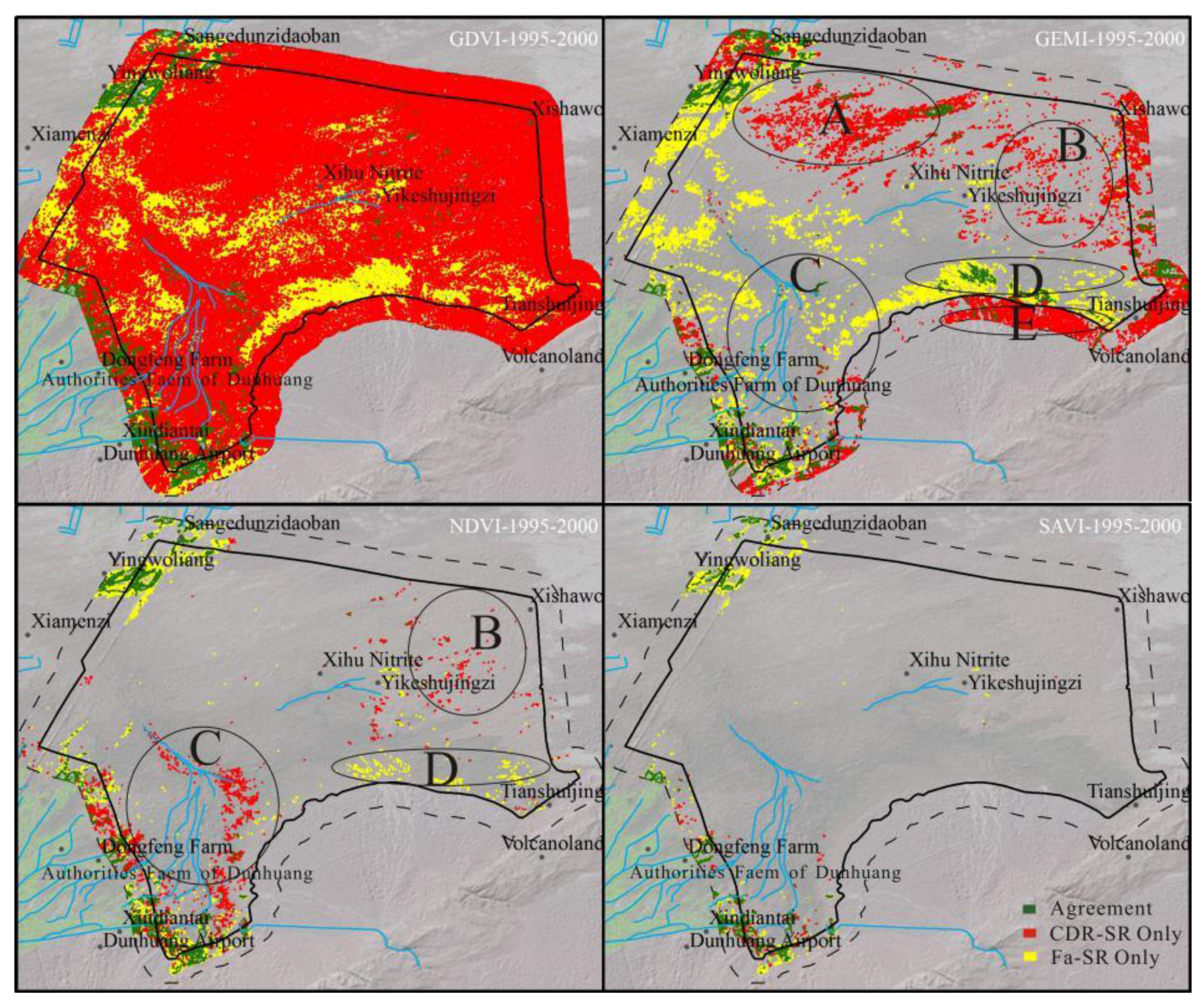
Figure 5.
Maps of inconsistencies in the pixels classified as changed for the period of 1990–1995 in the ΔGDVI, ΔGEMI, ΔNDVI, and ΔSAVI images produced using the CDR-SR images and the Fa-SR images. Annotated regions F to H are referred to in the text.
Figure 5.
Maps of inconsistencies in the pixels classified as changed for the period of 1990–1995 in the ΔGDVI, ΔGEMI, ΔNDVI, and ΔSAVI images produced using the CDR-SR images and the Fa-SR images. Annotated regions F to H are referred to in the text.

Figure 6.
Changes in vegetation detected in each period from 1986 to 2015. The data of the oasis were described by Zhang et al. [11]. Annotated regions (a) to (f) are referred to in the text.
Figure 6.
Changes in vegetation detected in each period from 1986 to 2015. The data of the oasis were described by Zhang et al. [11]. Annotated regions (a) to (f) are referred to in the text.
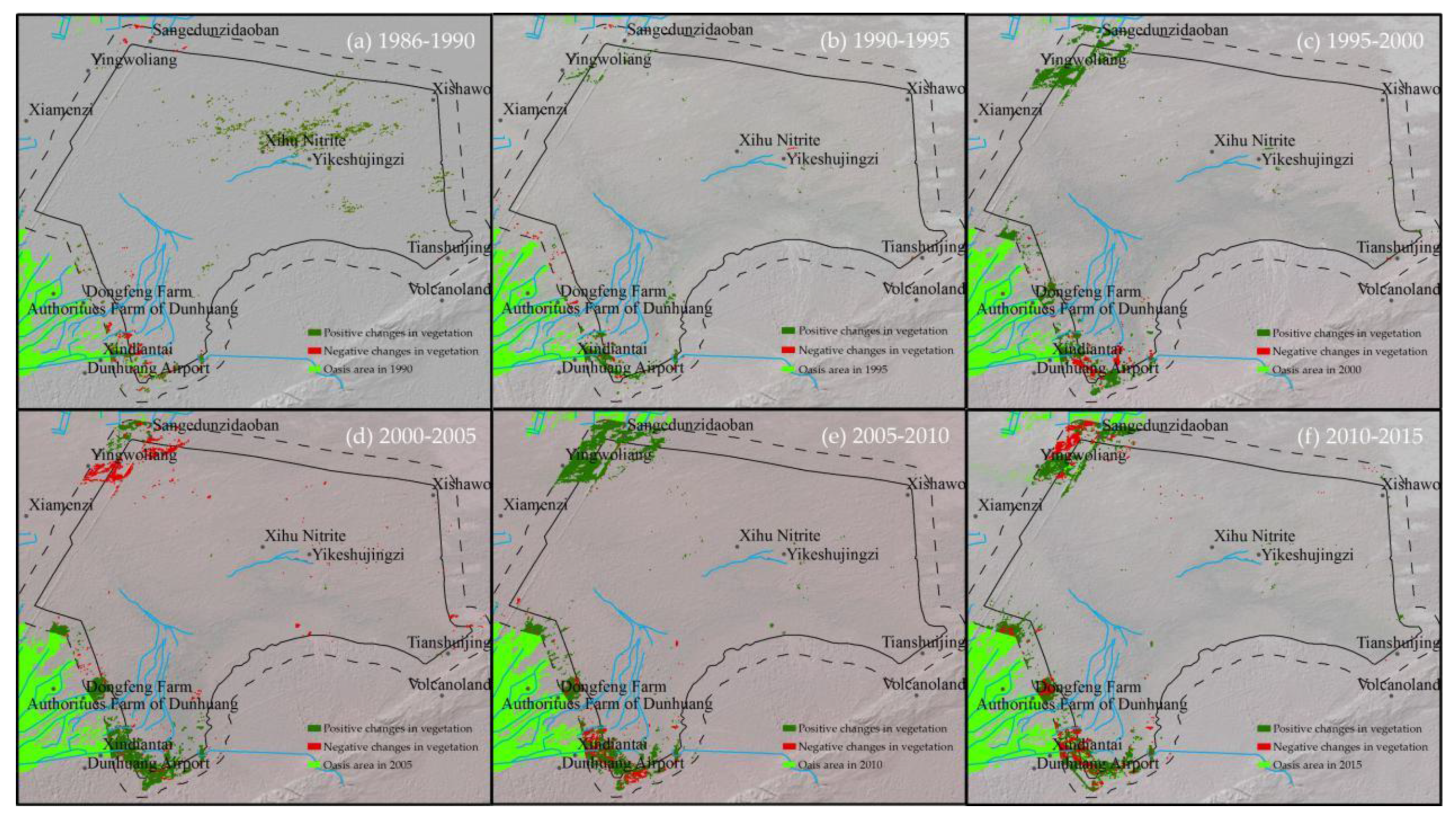
Figure 7.
The area of vegetation changes during 1986–2015; the horizontal axis tick labels indicate the pairs of the two years (centuries are not shown).
Figure 7.
The area of vegetation changes during 1986–2015; the horizontal axis tick labels indicate the pairs of the two years (centuries are not shown).

Table 1.
Landsat acquisition date and sensor type.
| Sensor | Path/Row | Imaging Time | Cloud Cover (%) |
|---|---|---|---|
| Landsat TM5 | 137/32 | 1986-07-23 | 0.05 |
| Landsat TM5 | 137/32 | 1990-08-19 | 8.38 |
| Landsat TM5 | 137/32 | 1995-08-17 | 0.15 |
| Landsat TM5 | 137/32 | 2000-07-29 | 0 |
| Landsat TM5 | 137/32 | 2005-07-11 | 11.04 |
| Landsat TM5 | 137/32 | 2010-07-09 | 7.66 |
| Landsat OLI8 | 137/32 | 2015-08-08 | 0.52 |
© 2017 by the authors. Licensee MDPI, Basel, Switzerland. This article is an open access article distributed under the terms and conditions of the Creative Commons Attribution (CC BY) license (http://creativecommons.org/licenses/by/4.0/).
Share and Cite
MDPI and ACS Style
Zhang, X.; Xie, Y. Detecting Historical Vegetation Changes in the Dunhuang Oasis Protected Area Using Landsat Images. Sustainability 2017, 9, 1780. https://doi.org/10.3390/su9101780
AMA Style
Zhang X, Xie Y. Detecting Historical Vegetation Changes in the Dunhuang Oasis Protected Area Using Landsat Images. Sustainability. 2017; 9(10):1780. https://doi.org/10.3390/su9101780
Chicago/Turabian StyleZhang, Xiuxia, and Yaowen Xie. 2017. "Detecting Historical Vegetation Changes in the Dunhuang Oasis Protected Area Using Landsat Images" Sustainability 9, no. 10: 1780. https://doi.org/10.3390/su9101780
Note that from the first issue of 2016, this journal uses article numbers instead of page numbers. See further details here.