Distributed Demand Side Management with Battery Storage for Smart Home Energy Scheduling

Abstract

The role of Demand Side Management (DSM) with Distributed Energy Storage (DES) has been gaining attention in recent studies due to the impact of the latter on energy management in the smart grid. In this work, an Energy Scheduling and Distributed Storage (ESDS) algorithm is proposed to be installed into the smart meters of Time-of-Use (TOU) pricing consumers possessing in-home energy storage devices. Source of energy supply to the smart home appliances was optimized between the utility grid and the DES device depending on energy tariff and consumer demand satisfaction information. This is to minimize consumer energy expenditure and maximize demand satisfaction simultaneously. The ESDS algorithm was found to offer consumer-friendly and utility-friendly enhancements to the DSM program such as energy, financial, and investment savings, reduced/eliminated consumer dissatisfaction even at peak periods, Peak-to-Average-Ratio (PAR) demand reduction, grid energy sustainability, socio-economic benefits, and other associated benefits such as environmental-friendliness.

1. Introduction

The smart grid is envisioned to offer grid reliability, sustainability, efficiency, and security with better consumer participation and environmental friendliness. It will be an environment with bi-directional flow of power and information between utilities and consumers through enabling information and communication technologies [1].

Demand Side Management (DSM) is an essential component for smart grid goals to be achieved. Recent DSM studies [2,3,4,5,6,7,8], have presented some techniques for appliance energy consumption scheduling, peak demand reduction (PDR), and Peak-to-Average-Ratio (PAR) demand reduction with some level of consumer preferences.

The need to enhance power supply stability in the grid has led to exploring additional power supply sources such as Distributed Energy Resources (DERs), for example, wind turbines and solar panels, and Distributed Energy Storage (DES), for example, batteries, electric vehicles, and fuel cells. Energy storage in batteries for use on consumer premises is promising due to recent development in battery designs with features such as larger storage capacities, longer discharge period, and better charging and discharging efficiencies [6].

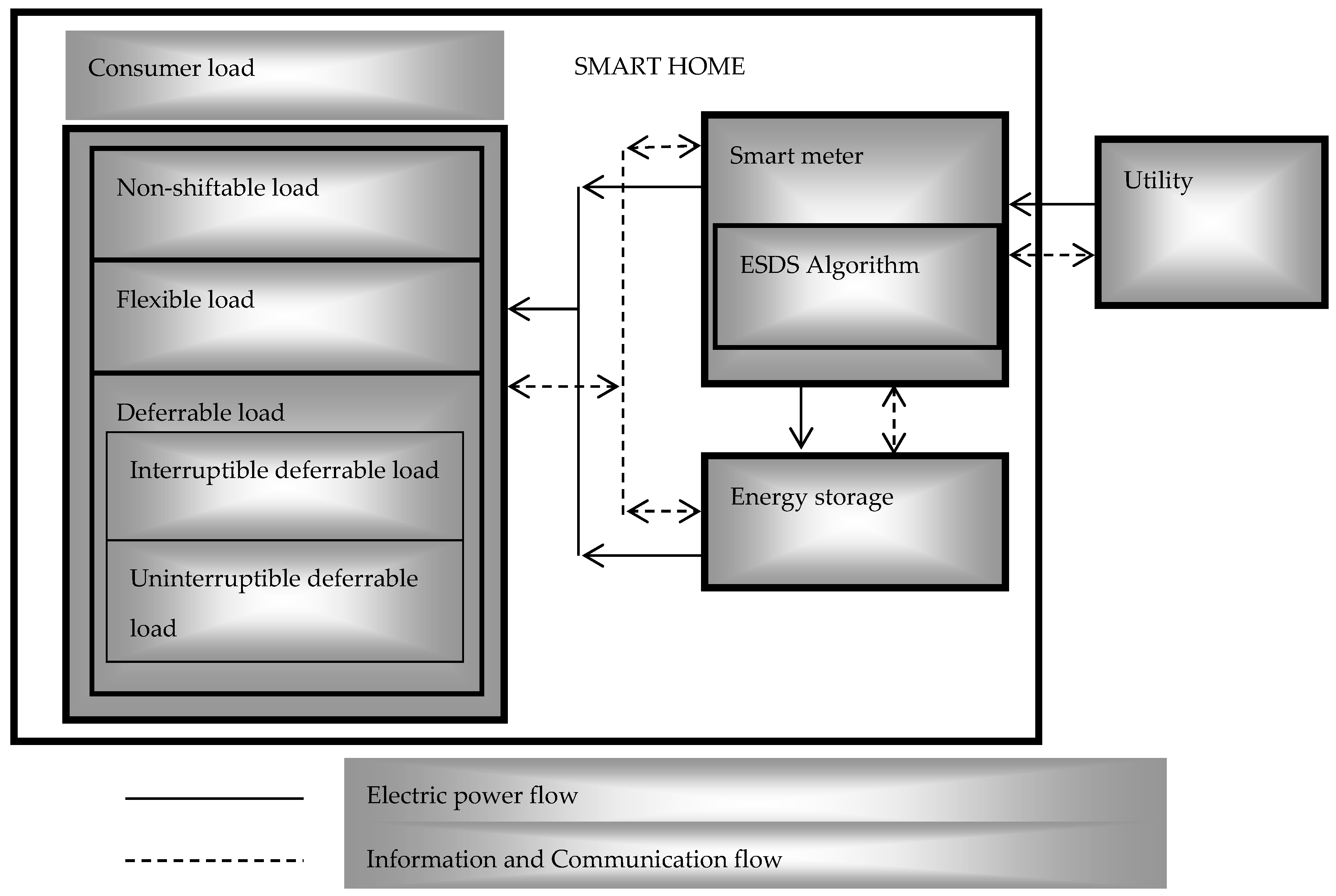
Generally, when consumers’ consumption is scheduled, it is the peak period demand that is often shifted to non-peak period, thereby leading to consumer dissatisfaction/discomfort. Hence, this work intends, through its proposed DSM algorithm, to offer PDR benefits to the utility with reduced or negligible peak period demand dissatisfaction to consumers, by optimizing energy supply and demand in consumer premises through the incorporation of an in-home DES device. The proposed Energy Scheduling and Distributed Storage (ESDS) algorithm will carry out energy consumption, storage, and expenditure optimization in the smart homes equipped with an in-home DES device. The ESDS algorithm optimizes energy demand and supply in the home between the grid and battery depending on grid energy price and consumer preferences. The ESDS optimization problem was formulated using convex programming and can be installed into smart meters on consumers’ premises.

The proposed algorithm would offer energy expenditure reduction and affordability, better consumer satisfaction even at peak periods, utility savings on peaker plants, reduced PAR demand and reduced carbon dioxide (CO₂) emissions from peaker plants. Consumer’s privacy is also offered, since the consumers do not need to send their energy consumption schedule to everyone within the network, but to the utility only. This would, in essence, reduce signaling complexity and communication investment costs in the smart grid infrastructure.

The rest of the work is organized as follows. Some related literature on DES for DSM applications are presented in Section 2, while a description of the ESDS model is presented in Section 3. The ESDS problem formulation is in Section 4. Section 5 contains the simulation results and discussions while Section 6 contains the conclusion of the work.

2. Related Work

Energy storage batteries can be installed into consumers’ premises as standalone or grid-connected sources. Energy storage capabilities in DSM programs have been studied in some literature [2,6,8,9]. The work in [2,6] applied parallel DSM algorithms to optimize energy consumption. However, modeling of distributed generators with capacity to trade with the grid in order to reduce consumer payments for electricity and utility cost, but with a penalty if consumer’s load was higher than a level compared with that of other consumers in the network was presented in [2]. The work thereby constrains a consumers’ satisfaction to be dependent on other consumers’ consumption. In [6], the authors presented a distributed energy consumption and storage optimization algorithm to minimize consumer energy payments while allowing the consumers to update their strategies simultaneously, but without modeling consumer satisfaction and a detailed battery storage profile with parameters that could influence the results presented. In [8], a model for grid, distributed energy production and storage with an independent centrally controlled day-ahead optimization algorithm was proposed for consumers. However, the selfish optimization of individual consumer’s consumption in such a pricing system where aggregate demand influences overall energy price may pose an unfair energy price on some consumers in the network. A large scale Energy Storage System (ESS) was proposed in [9] for centralized congestion relief in a smart grid using a real-time optimal dispatch algorithm, but it could be incapacitated by low penalty factors and imperfect forecast of energy price and congestion signals. Also, in order to coordinate charging multiple batteries in different houses and to prevent grid overload due to additional battery load, an agent-based micro storage management algorithm was proposed in [10] using game theory.

Although many algorithms have proposed energy consumption scheduling algorithms for DSM, the proposed ESDS algorithm in this paper attempts to optimize consumer energy consumption and demand satisfaction simultaneously in smart homes. It further applies its dissatisfaction model according to the nature of the appliance. Mathematical optimization techniques are promising in the design of DSM programs [4,5,6,7,11], and it will be employed also in this work to model the proposed ESDS problem.

3. Description of ESDS Architecture

Each smart home considered in this work is assumed to possess an energy storage device (e.g., batteries) installed within its premise as illustrated in Figure 1. The energy scheduling information from the consumers are sent to the utility via the Data Aggregation Point (DAP), while pricing and billing information from the utility are also passed through the same channel to the consumers.

The appliances can either be powered from the grid or the battery depending on the cost of electricity at a particular time. Therefore, the model is designed such that the household uses energy primarily from the grid at low tariff periods and primarily from the batteries at high tariff periods. Furthermore, the battery is only scheduled to be charged from the grid at low price periods.

In a Time-of-Use (TOU) pricing scenario, the cost of energy consumption to the consumer is higher at peak times than non-peak times and also higher during winter than summer as shown in

Table 1. Time-of-Use (TOU) tariff for single phase domestic customers.

Period	Weekday Time (h)	Summer (c/kWh)	Winter (c/kWh)
Peak	07:00–10:00, 18:00–20:00	109.89	262.09
Standard	10:00–16:00, 20:00–22:00	86.93	104.65
Off-peak	23:00–05:00	68.39	73.38

[12] for week days. The whole day is off-peak pricing on Sundays while Saturdays have standard pricing for 07:00–12:00 h and 18:00–20:00 h, and the rest of the day is off-peak pricing [12]. A higher disparity occurs between summer and winter peak period tariffs than between other period tariffs. This was intended by the utility to force reduced demand from the grid during the peak periods of winter. Off-peak and standard periods are categorized together in this work as non-peak periods.

4. ESDS Problem Formulation

The ESDS problem formulation is detailed in this section.

4.1. Household Appliance Consumption Model

Let every smart home, $a\in \mathbb{A},\mathrm{where}\mathbb{A}=\left[1,2,\dots ,A\right]$ in the smart grid with in-home storage facilities possess non-shiftable and shiftable smart appliances. A non-shiftable appliance, $i\in \mathbb{I}$, is assumed to be a non-schedulable appliance (e.g., lighting, cooking, television, etc.). The shiftable appliances are further classified as flexible (power-shiftable) and deferrable (time-shiftable) appliances. A flexible appliance, $j\in \mathbb{J}$, is a smart appliance whose power consumption levels can be shifted (e.g., air-conditioner, space heater, etc.) in response to tariff and consumer demand satisfaction, while a deferrable appliance is a smart appliance whose energy consumption can be shifted in time in response to tariff and consumer demand satisfaction. A deferrable load can either be uninterruptible or interruptible. The uninterruptible deferrable load (e.g., dish washer, washing machine, etc.), $f\in \mathbb{F}$, is the type of load whose operation start times can be shifted in time, but same duration of operation is still experienced by the appliance. While the interruptible deferrable appliance (e.g., pool pump, clothes dryer, etc.), $l\in \mathbb{L},$ can have certain tasks interrupted during operation and scheduled to continue later. Therefore, let all the household smart appliances belong to $\mathbb{G}=\mathbb{I}{\displaystyle \cup }\mathbb{J}{\displaystyle \cup }\mathbb{F}{\displaystyle \cup }\mathbb{L}=\mathbb{I}{\displaystyle \cup }\mathbb{H},$ where $\mathbb{H}=\mathbb{J}{\displaystyle \cup }\mathbb{F}{\displaystyle \cup }\mathbb{L}$. The total load, $x_{a,t}$, of consumer $a$ at any time, $t\in \mathbb{T}$, where $\mathbb{T}=\left[1,2,\dots ,\mathrm{ȶ}\right],$ is given by:

$$x_{a,t}={\displaystyle \sum }_{i\in \mathbb{I}}{x}_{a,i,t}+{\displaystyle \sum }_{h\in \mathbb{H}}{x}_{a,h,t},h=\left\{j,f,l\right\}, \forall t\in \mathbb{T}.$$

(1)

Also, the total schedulable load, $x_{a,h,t},$ by all schedulable appliances, $h\in \mathbb{H},$ at a given time $t$ is expressed as:

$$x_{a,h,t}={\displaystyle \sum }_{j\in \mathbb{F}}{x}_{a,j,t}+{\displaystyle \sum }_{f\in \mathbb{F}}{x}_{a,f,t}+{\displaystyle \sum }_{l\in \mathbb{E}}{x}_{a,l,t}, \forall t\in \mathbb{T}.$$

(2)

The load vector for all households in the smart grid, $x=\left[x_1,x_2,...,x_a,\dots ,x_A\right],$ and the daily load vector for each consumer, $x_a={\left[x_{a,1},x_{a,2},...,x_{a,\mathrm{ȶ}}\right]}^{\prime }$, while its total daily load is expressed as:

$$x_a= {\displaystyle \sum }_{t\in \mathbb{T}}{x}_{a,t}, \forall a\in \mathbb{A}.$$

(3)

Assume the feasible period of operation, ${\mathcal{T}}_{a,g},$ of any appliance, $g,$ in the household has a start time, $t_{a,g,}^s$ and end time, $t_{a,g}^e$, where ${\mathcal{T}}_{a,g}=\left\{t\right|t_{a,g}^s\le t\le t_{a,g}^e\}$, $g=\{i,j,f,l$}, $\forall g\in \mathbb{G}$. Then, total energy, $e_{a,g},$ consumed by any appliance, $g\in \mathbb{G},$ during its feasible period of operation is given by:

$$e_{a,g}=\{\begin{array}{c}{\displaystyle {\displaystyle \sum }_{t_{a,g}^s}^{t_{a,g}^e}}{x}_{a,g,t}, \forall t\in \mathbb{T}, g=\left\{i,j,f,l\right\}, \forall g\in \mathbb{G}\hfill \\ 0, \forall t\in \mathbb{T}\backslash {\mathcal{T}}_{a,g}, g=\left\{i,j,f,l\right\}, \forall g\in \mathbb{G}\hfill \end{array}.$$

(4)

Therefore, the energy balance in the smart grid is given by:

$${\displaystyle \sum }_{t\in \mathbb{T}}{x}_t={\displaystyle \sum }_{a\in \mathbb{A}}{\displaystyle \sum }_{g\in \mathbb{G}}{e}_{a,g},g=\left\{i,j,k,l\right\}$$

(5)

Power level constraint for each smart appliance, $g\in \mathbb{G},$ is in a smart home is given as:

$$x_{a,g}^{min}\le x_{a,g,t}\le x_{a,g}^{max},g=\left\{i,j,f,l\right\}, \forall t\in {\mathcal{T}}_{a,g},$$

(6)

where $x_{a,g}^{min}$ and $x_{a,g}^{max}$ define the minimum power level (off or standby mode) and maximum power level of each smart appliance, respectively. Also, $x_{a,g}^{min}\ge 0$ and $x_{a,g}^{max}>0$.

4.2. Consumer Dissatisfaction Cost Model

4.2.1. Power Shiftable Loads

The consumer will incur some dissatisfaction cost each time it attempts to shift the power level of its flexible loads from its nominal load, $u_{a,j,t},$ to an actual load, $x_{a,j,t}$. If the degree of dissatisfaction of a flexible load that is tolerable to the consumer is ${\alpha }_{a,j}$, then dissatisfaction cost, ${\overline{d}}_{a,j}^t,$ is expressed in (7) by modifying the satisfaction cost in [2]:

$${\overline{d}}_{a,j}^t={\alpha }_{a,j}\left(u_{a,j,t}{\theta }_t\left[1-{\left(\frac{x_{a,j,t}}{u_{a,j,t}}\right)}^{{\gamma }_t}\right]\right),\forall j\in \mathbb{J},$$

(7)

where $0\le {\alpha }_{a,j}\le 1$, ${\gamma }_t, {\theta }_t\in \mathbb{R}, {\gamma }_t<1$, and ${\gamma }_t{\theta }_t<0$. The values of ${\alpha }_{a,j},{\gamma }_t$ and ${\theta }_t$ are varied to model different levels of consumer dissatisfaction.

4.2.2. Time Shiftable Loads

This shall be considered for both uninterruptible and interruptible loads. The dissatisfaction cost of uninterruptible deferrable loads, ${\overline{d}}_{a,f}^t,$ in this model is expressed as a function of the delay/haste dissatisfaction in starting the task, and the measure of dissatisfaction tolerance, ${\alpha }_{a,f},$ of such delay/haste to the consumer is given as:

$${\overline{d}}_{a,f}^t={\alpha }_{a,f}\left|t_{a,f}^{s,s}-t_{a,f}^s\right|,0\le {\alpha }_{a,f}\le 1,\forall f\in \mathbb{F},$$

(8)

where $t_{a,f}^{s,s}$ and $t_{a,f}^s$ are the actual start time and nominal start time of the uninterruptible deferrable load, respectively. A high delay/haste tolerance factor, ${\alpha }_{a,f},$ indicates the consumer is able to tolerate high dissatisfaction due to the delay/haste task execution and vice versa. Hence, ${\alpha }_{a,f}$ can be used to model different levels of consumer’s dissatisfaction of uninterruptible deferrable loads. If the operation was scheduled by the ESDS to start before the nominal task start time, it is considered a haste task, while if it occurs after, it is regarded as a delay task. For uninterruptible deferrable loads, the actual feasible operation period ${\mathcal{T}}_{a,f}^s=\{t|t_{a,f}^{s,s}\le t\le t_{a,f}^{e,s}\}$. To ensure that the operation of an uninterruptible smart appliance continues once it starts without being interrupted, then the actual end time, $t_{a,f}^{e,s}$, for the scheduled task is constrained by:

$$t_{a,f}^{e,s}\ge t_{a,f}^{s,s}+{\eta }_{a,f},\forall f\in \mathbb{F}, \forall t\in \mathbb{T},\forall a\in \mathbb{A}.$$

(9)

where nominal task duration ${\eta }_{a,f}=\left|t_{a,f}^e-t_{a,f}^s\right|$.

For interruptible deferrable loads, the actual feasible period ${\mathcal{T}}_{a,l}^s=\{t|t_{a,l}^{s,s}\le t\le t_{a,l}^{e,s}\}={\mathcal{T}}_{a,l}^{s_1}+{\mathcal{T}}_{a,l}^{s_2}+\dots +{\mathcal{T}}_{a,l}^{s_q}$, where ${\mathcal{T}}_{a,l}^{s_1},{\mathcal{T}}_{a,l}^{s_2},\dots ,{\mathcal{T}}_{a,l}^{s_q}$ are possible durations of q number of scheduled sub-tasks within the entire task duration. If the actual entire task duration ${\eta }_{a,l}^s=|t_{a,l}^{e,s}-t_{a,l}^{s,s}|$ and the nominal task duration ${\eta }_{a,l}=|t_{a,l}^e-t_{a,l}^s|,$ then the dissatisfaction cost, ${\overline{d}}_{a,l}^t,$ on interruptible deferrable load is also related with its dissatisfaction tolerance factor, ${\alpha }_{a,l},$ by:

$${\overline{d}}_{a,l}^t={\alpha }_{a,l }\left|{\eta }_{a,l}-{\eta }_{a,l}^s\right|, 0\le {\alpha }_{a,l}\le 1,\forall l\in \mathbb{L}$$

(10)

The values of ${\alpha }_{a,j}$, ${\alpha }_{a,f},$ and ${\alpha }_{a,l}$ are adjustable and can vary from one appliance to another and also from one consumer to another. The total hourly dissatisfaction cost, ${\overline{d}}_a^t,$ in a consumer premise following from (7), (8), and (10) is given as:

$${\overline{d}}_a^t={\overline{d}}_{a,j}^t+{\overline{d}}_{a,f}^t+{\overline{d}}_{a,l}^t, \forall a\in \mathbb{A}.$$

(11)

The total daily dissatisfaction cost $\overline{d_a}={\displaystyle \sum }_{t\in \mathbb{T}}{\overline{d}}_a^t.$ The total dissatisfaction is measured in kWh because it is a measure of dissatisfaction in energy consumption by the consumer.

4.3. Battery Storage Model

Let $b_{a,t}$ be the energy stored in the battery at any time $t\in \mathbb{T}$ in the premise of consumer $a\in \mathbb{A}$. The daily energy storage scheduling vector $b_a={\left[b_{a,1},b_{a,2},\dots ,b_{a,\mathrm{ȶ}}\right]}^{\prime }$. Also, $b_{a,t}=b_{a,t}^{+}-b_{a,t}^{-}$, where $b_{a,t}^{+}$ is the energy charging profile and $b_{a,t}^{-}$ is the energy discharging profile, and $b_{a,t}^{+},b_{a,t}^{-}\ge 0$. Example of specifications for in-home batteries can be found in [13].

Due to the conversion losses of the storage device, the charging efficiency ${\beta }_a^{+}$ and discharging efficiency ${\beta }_a^{-}$ fulfil conditions $0<{\beta }_a^{+}\le 1$ and ${\beta }_a^{-}\ge 1,$ respectively [8]. Therefore, if $b_{a,t}^{+}$ is the amount of energy consumed from the grid to charge the battery, it is only effectively charged with ${\beta }_a^{+}{b}_{a,t}^{+}$ amount of energy. Likewise if $b_{a,t}^{-}$ is required to be discharged from the battery to the smart appliances in the home, then only ${\beta }_a^{-}{b}_{a,t}^{-}$ is effectively discharged from the battery. The charging and discharging efficiency vector ${\mathsf{\beta }}_a={\left[{\beta }_a^{+},-{\beta }_a^{-}\right]}^{\prime }$ and per-slot storage scheduling vector $b_{a,t}={\left[b_{a,t}^{+},b_{a,t}^{-}\right]}^{\prime }$. Then energy charged/discharged ${\mathsf{\beta }}_a^{\prime }{b}_{a,t}$ at time $t\in \mathbb{T}$ is related to the maximum charging rate $b_a^{max}$ by:

$${\mathsf{\beta }}_a^{\prime }{b}_{a,t}\le b_a^{max}$$

(12)

The energy leakage rate ${\lambda }_a$ of the battery is the rate of decrease in charge level on no-load and is bounded as $0<{\lambda }_a\le 1$. Hence, the battery charge level $q_{a,t}$ reduces by ${\lambda }_a{q}_{a,t}$ at time $t+1$, but is related to the previous charge level $q_{a,t-1}$ at time $t-1$ by:

$$q_{a,t}=q_{a,t-1}\left(1-{\lambda }_a\right)+{\mathsf{\beta }}_a^{\prime }{b}_{a,t}$$

(13)

The charge level $q_{a,t}$ of the battery is bounded as:

$$0\le q_{a,t}\le b_{cap}$$

(14)

where $b_{cap}$ is the battery capacity. Therefore, following from (13) and (14), $b_{a,t}$ can be constrained as:

$$-q_{a,t-1}\left(1-{\lambda }_a\right)\le {\mathsf{\beta }}_a^{\mathrm{T}}{b}_{a,t}\le b_{cap}-q_{a,t-1}\left(1-{\lambda }_a\right)$$

(15)

Also, $q_{a,t}$ is related to the initial charge level $q_{a,t_0}$ of the battery and its storage profilesby:

$$q_{a,t}=q_{a,t_0}\left(1-{\lambda }_{a,t}\right)+{\displaystyle \sum }_{t=t_0}^t{\lambda }_{a,t-t_0}{\mathsf{\beta }}_a^{\mathrm{T}}{b}_{a,t}$$

(16)

4.4. Grid Energy Consumption Model

The per-timeslot demand, $Y_{a,r}^t,$ and total daily demand, $Y_{a,r},$ from the grid are given by (17) and (18):

$$Y_{a,r}^t=\{\begin{array}{c}{x}_{a,t}+b_{a,t}^{+} , \forall t\in t_{np},t_{np}\subset \mathbb{T}\hfill \\ {\left(x_{a,t}-q_{a,t}\right)}^{+}, \forall t\in t_p, t_p\subset \mathbb{T}\hfill \end{array},$$

(17)

$$Y_{a,r}={\displaystyle \sum }_{t\in \mathbb{T}}{Y}_{a,r}^t,\forall t\in \mathbb{T}, \forall a\in \mathbb{A},$$

(18)

respectively, where $t_{np}$ and $t_p$ are sets of non-peak and peak periods, respectively. The ESDS algorithm uses energy price to determine the source of electricity to consumer appliances at every time $t\in \mathbb{T}$. It reads the energy stored in the battery at the price that the energy was brought from the grid and compares it with the utility block TOU price and chooses the lower price in order to minimize the consumer’s energy expenditure. Hence, more consumer load is permitted to be scheduled for the peak period within the capacity of the energy stored in the battery. Therefore, the daily grid energy demand vector $Y_{a,r}={\left[Y_{a,r}^1,Y_{a,r}^2,\dots ,Y_{a,r}^{\mathrm{ȶ}}\right]}^{\prime }$. The total demand from the grid by a household is bounded as:

$$0\le Y_{a,r}^t\le Y_{a,r}^{t,max},\forall t\in \mathbb{T},\forall a\in \mathbb{A}$$

(19)

The maximum load $Y_{a,r}^{t,max}$ is dependent upon the fuse/line capacity or as determined by the utility for each household. Also, since the batteries are not feeding the grid then:

$$x_{a,t}+b_{a,t}\ge 0,\forall t\in \mathbb{T}, \forall a\in .$$

(20)

4.5. Energy Expenditure Model

Energy expenditure to the consumers, $C_a^t$, is a function of the total energy consumed from the grid$, Y_{a,r}^t,$ and the TOU price, $P_t$, where $P={\left[P_1, P_2, \dots , P_{\mathrm{ȶ}}\right]}^{\text{'}}$ at every time $t$. Therefore, the hourly and daily energy expenditure, $C_a^t$ and $C_a,$ are, respectively, given as follows:

$$C_a^t=P_t{Y}_{a,r}^t,$$

(21)

$$C_a={\displaystyle \sum }_{\forall t\in \mathbb{T}}{C}_a^t.$$

(22)

4.6. The ESDS Optimization Problem

The objective function in the ESDS algorithm is to minimize total demand from grid, energy expenditure, and dissatisfaction cost for each consumer. A convex programming problem was formulated as shown in (23), which can be solved using the interior point method [14]:

$$\begin{array}{c}\underset{C_a^t,{\overline{d}}_a^t \in \mathbb{R}}{min}{C}_a^t+{\overline{d}}_a^t\\ \mathrm{s}.\mathrm{t}.\left(1\right), \left(4\right)–\left(6\right), \left(9\right),\left(12\right), \left(14\right)–\left(17\right), \left(19\right), \left(20\right)\end{array}$$

(23)

4.7. PAR Demand Model

The effect of the ESDS algorithm was also investigated on PAR demand since it has potential to reduce peak period demand from the grid. The PAR demand is given by:

$$\mathrm{PAR}=\frac{\mathrm{Peak}\mathrm{demand}\mathrm{from}\mathrm{grid}}{\mathrm{Average}\mathrm{demand}\mathrm{from}\mathrm{grid}}=\frac{\underset{t\in \mathbb{T}}{max}{{\displaystyle \sum }}_{a\in \mathbb{A}}{Y}_{a,r}^t}{\frac{1}{{ȶ}}{{\displaystyle \sum }}_{a\in \mathbb{A},t\in \mathbb{T}}{Y}_{a,r}^t}$$

(24)

Since the denominator of (24) is approximately constant, then (24) can be simplified and solved as a linear program using the simplex method [15].

5. Simulation Results and Discussions

Household energy consumption data for 100 flats were obtained from Eskom Data Acquisition Department and fed into the ESDS algorithm for three scenarios namely: No DSM—Scenario 1, DSM without ESDS—Scenario 2, and DSM with ESDS—Scenario 3. Scenario 1 does not involve any optimization at all, as it is the obtained nominal consumption of the consumers. Scenario 2 solves (22) excluding all battery-related constraints, while Scenario 3 carries out the complete optimization problem as shown in (22).

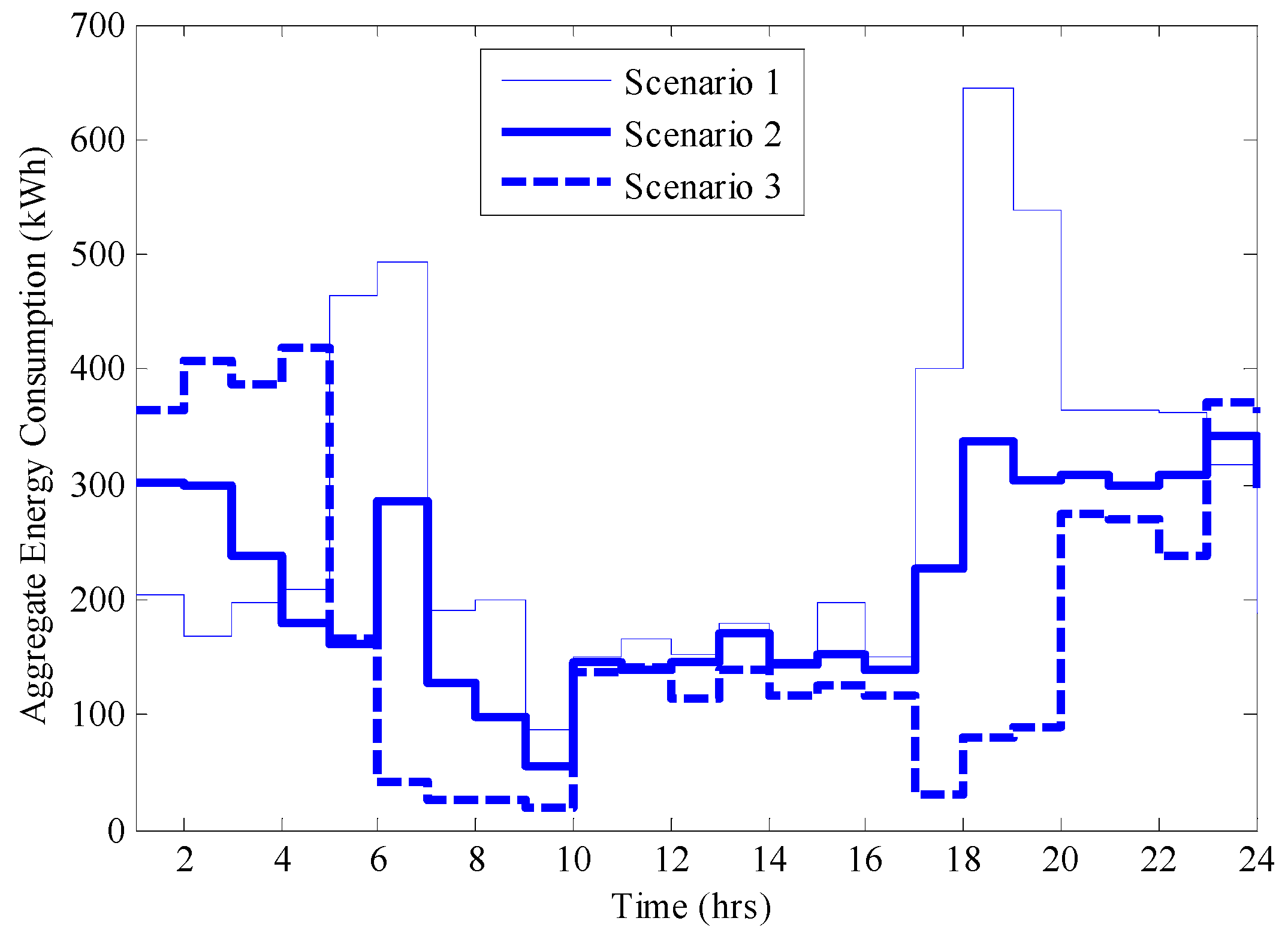
The results of average hourly energy consumption and expenditure from the grid for flats 5 and 12 chosen at random during summer are presented in Figure 2. It can be seen from Figure 2 that Scenarios 2 and 3 outperformed Scenario 1 for both flats because of the optimization scheduling involved in their algorithms. However, Scenario 3 outperformed Scenario 2 for both flats. The household consumed the least energy from the utility grid during morning and evening peak periods under Scenario 3 since the battery was the primary source of energy at peak periods. This, therefore, led to reduced energy consumption from the grid during peak periods and, consequently, reduced energy expenditure and increased financial savings for the consumers. The energy consumed from the battery at peak time by the scheduled appliances is the energy bought from the grid at a non-peak (off-peak and standard periods) TOU (low) prices. Also, the aggregate energy consumption profile for the one hundred households is presented in Figure 3.

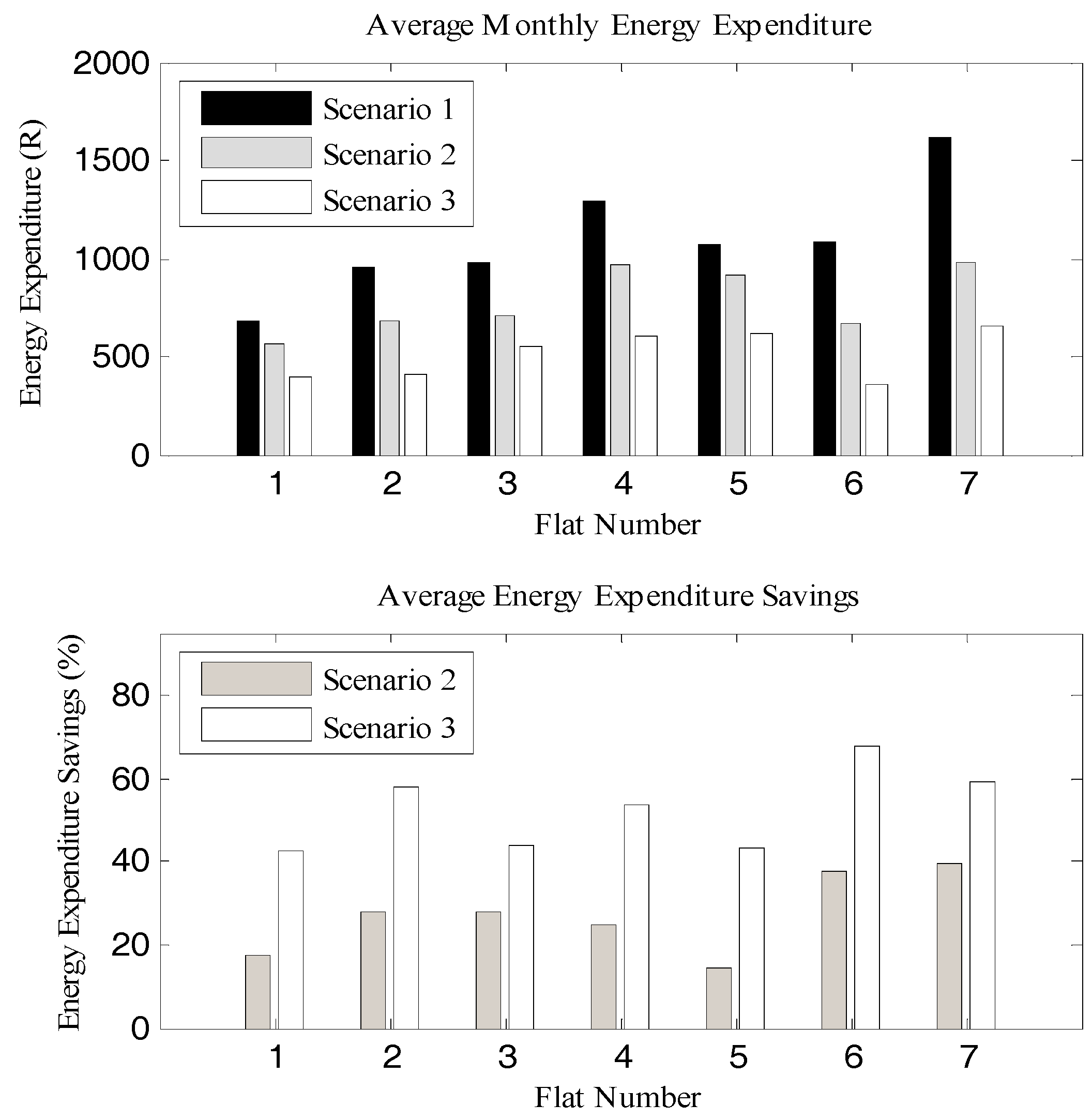
Hence, the Scenario 3 (ESDS) algorithm would offer the consumers more financial savings than the Scenario 2 algorithm. Average monthly energy expenditure in the local currency of South African rands (R) for seven out of the twenty consumers chosen at random is presented in Figure 4. Therefore, the consumers under Scenarios 2 and 3 algorithms were able to reduce their average energy expenditure, compared to Scenario 1. However, the financial savings on energy expenditure was higher for the consumers in Scenario 3 than for those in Scenario 2 due to the possession of DES in the consumers’ premises. The average monthly financial savings for all the households in Scenarios 2 and 3 were 27% and 53%, respectively. The battery payback periods are directly related to the amount of energy consumption and expenditure savings. The payback period on battery investment differ from one consumer to another within Scenario 3, and this depends on how much energy is scheduled for battery supply in the household.

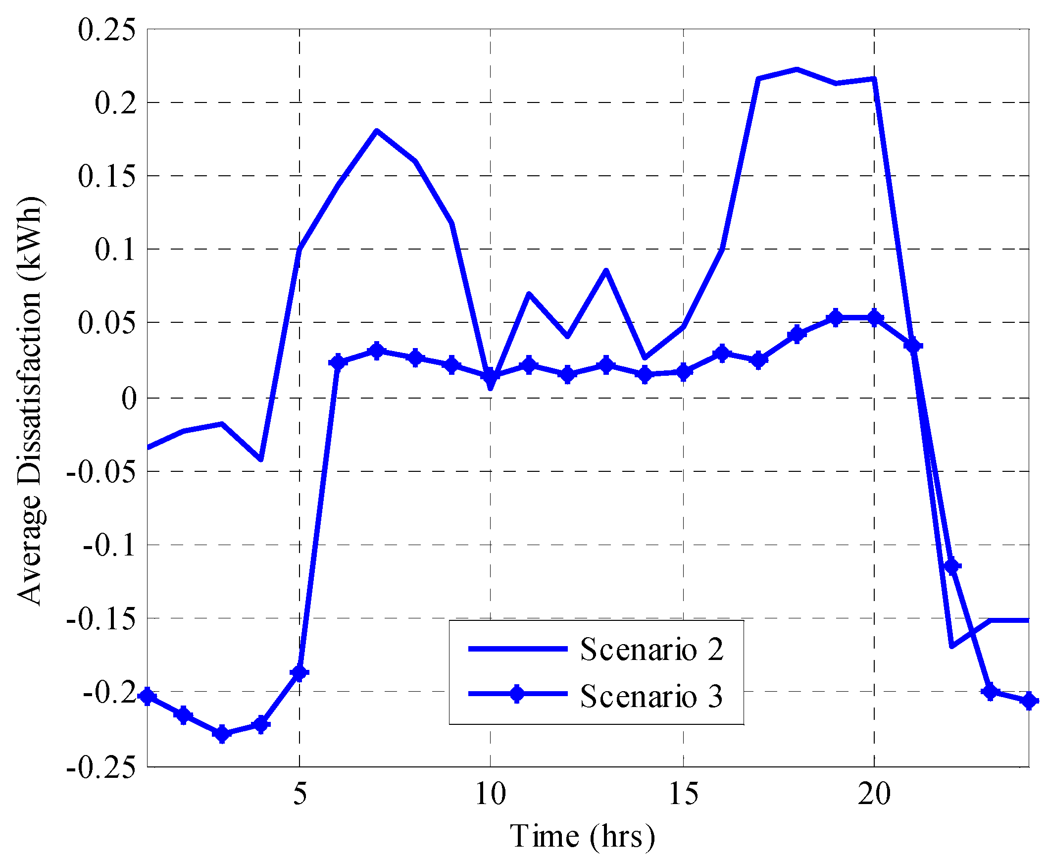
Energy consumption scheduling on consumers’ premises has known advantages, but not without the disadvantage of demand dissatisfaction. However, the implementation of DES in an ESDS algorithm proposes reduced or negligible demand dissatisfaction cost. In terms of the dissatisfaction cost, it was observed that Scenario 3 offered lower dissatisfaction to consumers than Scenario 2 especially at peak periods. This is because the consumers under Scenario 3 had purchased energy from the grid at non-peak times (low energy price periods) and stored it in their batteries. This stored energy is primarily discharged locally to household appliances during morning and evening peak periods, and thereby mitigates the peak period demand dissatisfaction that characterizes the Scenario 2 scheduling algorithm like other DSM energy scheduling algorithms in the literature [4,5,7]. The effect of DSM scheduling in Scenarios 2 and 3 on dissatisfaction cost is shown in Figure 5. Dissatisfaction cost was not considered for Scenario 1 because it was the consumer’s traditional nominal consumption without energy scheduling and, hence, has no demand dissatisfaction cost.

The flexible appliances generate positive, negative, and zero demand dissatisfaction, while the deferrable appliances generate either positive or zero dissatisfaction depending on the load scheduling. Positive total daily dissatisfaction is not desirable for maximized consumer’s welfare. The desirable total daily dissatisfaction, ${\overline{d}}_a,$ for a consumer should be ${\overline{d}}_a\le 0$ for consumer’s maximum social welfare and minimized energy expenditure. The simulation results showed that the average daily dissatisfaction for Scenarios 2 and 3 were 1.386 kWh and −1.065 kWh, respectively. This implies that the integration of the battery into the consumer’s premise offered reduced or negligible dissatisfaction to the consumers.

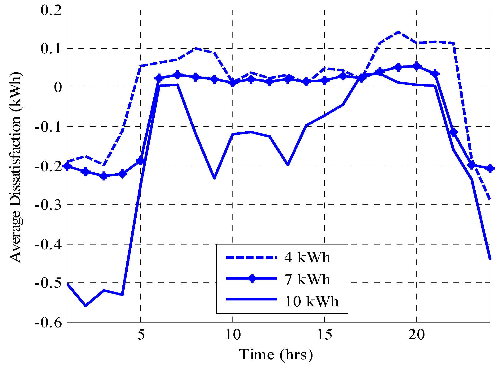
Also, further sensitivity analysis was carried out to investigate the effect of battery capacity on consumer’s dissatisfaction. It was discovered that the higher the battery capacity acquired by a consumer, the less it will be dissatisfied by appliance scheduling with respect to its average peak period demand. However, battery capacity cannot indefinitely increase; otherwise, the law of diminishing returns would set in for financial savings and battery pay-back period. The battery capacity assumed initially in the simulation was 7 kWh. Therefore, the effects of 4 kWh and 10 kWh battery capacities on demand dissatisfaction were studied, and the results found are presented in Figure 6. The average daily demand dissatisfaction obtained were 0.063 kWh, −1.265 kWh, and −4.217 kWh for the 4 kWh, 7 kWh, and 10 kWh batteries, respectively. This implies that the 10 kWh battery capacities would not be economical for the consumers whose consumption data was simulated in this work due to very high satisfaction. However, the consumer can choose between the 4 kWh and 7 kWh batteries depending on their tolerance for dissatisfaction. From interpolation, it was observed that zero dissatisfaction can be achieved with approximately 5 kWh battery capacity. Too high satisfaction is not cost efficient because optimal satisfaction, expenditure savings, and good battery health intercept at zero dissatisfaction.

Hence, there is a need for consumers to seek technical advice before purchasing an in-home energy storage device for optimized satisfaction and energy expenditure. Also, the total daily morning or evening peak period demand can be used to determine the size of battery capacity.

The state of health and degradation cost of any battery depends upon factors such as its lifetime throughput, roundtrip efficiency, and replacement cost, among others. While state of health reduces with battery usage, degradation cost increases with usage and, consequently, the level of satisfaction that the battery can offer to the consumers will also reduce with time and usage.

The average PAR demand for Scenarios 1, 2, and 3 were found to be 1.961, 1.675, and 1.154, respectively, which are less than the results obtained in [6]. Therefore, Scenario 3 would offer the utility grid better stability and reliability than others due to its lowest grid peak demand and PAR demand. Best satisfaction is obtained when dissatisfaction is zero. The more negative the dissatisfaction is, the lower the comparative advantage of a higher battery capacity on energy savings.

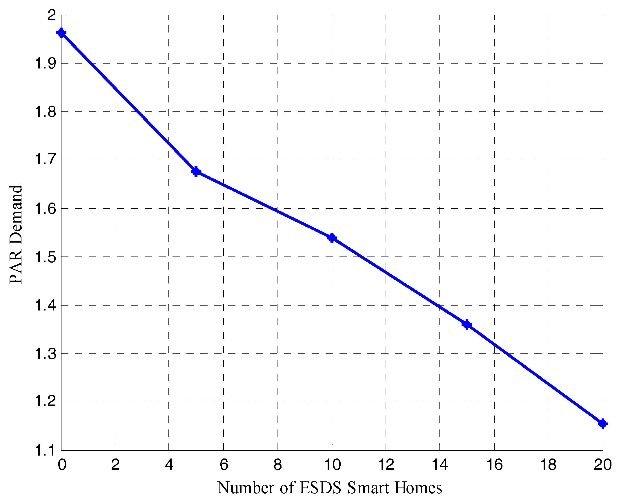
The relationship between number of ESDS smart homes in the smart grid and PAR demand was also investigated and the result is presented in Figure 7. This sensitivity analysis was carried out on PAR demand because it may not be a realistic assumption that all the smart homes in a smart microgrid or smart grid at large would have battery storage facilities installed in their premises for DSM purposes. And as can be seen from Figure 7, the higher the number of ESDS smart homes in a smart grid, the lower the PAR demand of the smart grid.

The relationship between battery capacity and aggregate PAR demand is presented in Figure 8, and it shows that the higher the battery capacity of the in-Home Energy Storage (iHES) device, the lower the aggregate PAR demand from the grid. This was simulated for no battery (i.e., 0 kWh), 4 kWh, 7 kWh, and 10 kWh battery capacities.

The computational complexity involved in the ESDS algorithm is not beyond what can be solved in polynomial real time with an average computational time of 1.15 s depending on computer configuration. It can also be implemented into an embedded energy controller chip. Work is on-going on that in our laboratory. Practical implementation of the algorithm will be presented in future work. Limited security risk may arise, however, from the utility during communication.

Although the ESDS algorithm was tested for a TOU pricing scenario, it can also find application in a Real Time Pricing (RTP) environment by upgrading its pricing and demand response intelligence. Fundamentally, utilities set real-time energy prices based on the aggregate demand obtained from load schedule or forecasting. Therefore, energy prices are high at high demand periods and low at low demand periods. Hence, since the ESDS algorithm could minimize $Y_{a,r}^t$, then it can also be used to obtain reduced grid energy consumption, energy price, and expenditure for RTP consumers also. The ESDS contributes to the sustainability of the grid and environment by reducing peak energy demand from the grid [16] and offering a low carbon footprint [17].

The payback period for consumers depends on level of energy savings, financial savings, and the healthiness of individual iHES devices. On the other hand, payback period for the manufacturer would depend on the rate of technology adoption, pricing scheme, and ease of implementation of the technology, among others. The continuous research and development in macro and micro-energy storage technologies show possibilities of a shorter payback period on investment for both consumers and manufacturers of storage devices in the smart grid.

6. Conclusions

This work has studied the effect of DES in a smart grid for reduction in consumer peak period demand dissatisfaction and energy expenditure by solving a convex optimization problem called the ESDS algorithm. Three scenarios were considered for analyses—No DSM (Scenario 1), DSM without ESDS (Scenario 2), and DSM with ESDS (Scenario 3). Scenario 3 enabled the consumers to consume energy during peak periods at the lower price (off-peak or standard period prices) from when the energy was initially bought from the grid and stored in the battery. Hence, little or no consumer demands were scheduled for consumption from the grid at peak periods, thereby enhancing consumers’ satisfaction. The numerical results showed that Scenario 3 outperformed the other scenarios in energy savings, financial savings, reduced and negligible peak period demand dissatisfaction, and PAR demand reduction. The high average financial savings (53%) experienced by the consumers can lead to speedy adoption of the technology and consequently reduce the payback period on investment for the manufacturer. The proposed ESDS algorithm can offer consumer privacy and reduced security risk because each smart meter communicates directly to the utility, but not to other participating consumers in the network. The ESDS algorithm is shown to be a consumer-friendly, grid-friendly, financial-friendly, societal-friendly, and environmental-friendly DSM solution for the smart grid. Although the ESDS model has been shown for residential consumers in this work, it can also be modified and applied to commercial and industrial users.

References

1. Longe, O.M.; Ouahada, K.; Ferreira, H.C.; Rimer, S. Wireless sensor networks and advanced metering infrastructure deployment in smart grid. In Proceedings of the International Conference on e-Infrastructure and e-Services for Developing Countries, Blantyre, Malawi, 25–27 November 2013; pp. 167–171.
2. Yang, P.; Chavali, P.; Gilboa, E.; Nehorai, A. Parallel load schedule optimization with renewable distributed generators in smart grids. IEEE Trans. Smart Grid 2013, 4, 1431–1441. [Google Scholar] [CrossRef]
3. Song, L.; Xiao, Y.; van der Schaar, M. Demand side management in smart grids using a repeated game framework. IEEE J. Sel. Areas Commun. 2014, 32, 1412–1424. [Google Scholar] [CrossRef]
4. Longe, O.M.; Ouahada, K.; Ferreira, H.C.; Rimer, S. Optimization of energy expenditure in smart homes under Time-of-Use pricing. In Proceedings of the 2015 IEEE Innovative Smart Grid Technologies-Asia (ISGT ASIA), Bangkok, Thailand, 3–6 November 2015; pp. 1–6.
5. Longe, O.M.; Ouahada, K.; Rimer, S.; Zhu, H.; Ferreira, H.C. Effective Energy Consumption Scheduling in Smart Homes. In Proceedings of the IEEE Africa Conference (AFRICON), Addis Ababa, Ethiopia, 14–17 September 2015; pp. 724–728.
6. Nguyen, H.K.; Song, J.B.; Han, Z. Distributed Demand Side Management with energy storage in smart grid. IEEE Trans. Parallel Distrib. Syst. 2015, 26, 3346–3357. [Google Scholar] [CrossRef]
7. Mohsenian-Rad, H.; Wong, V.W.S.; Jatskevich, J.; Schober, R.; Leon-Garcia, A. Autonomous Demand Side Management Based on Game-Theoretic Energy Consumption Scheduling for the Future Smart Grid. IEEE Trans. Smart Grid 2010, 1, 320–331. [Google Scholar] [CrossRef]
8. Atzeni, L.; Ordóñez, G.; Scutari, G.; Palomar, D.P.; Fonollosa, J.R. Demand-side management via distributed energy generation and storage optimization. IEEE Trans. Smart Grid 2013, 4, 866–876. [Google Scholar] [CrossRef]
9. Khani, H.; Zadeh, M.R.D.; Hajimiragha, A.H. Transmission congestion relief using privately owned large-scale energy storage systems in a competitive electricity market. IEEE Trans. Power Syst. 2016, 31, 1449–1458. [Google Scholar] [CrossRef]
10. Vytelingum, P.; Voice, T.D. Agent-based micro-storage management for the smart grid. In Proceedings of the 9th International Conference on Autonomous Agents and Multiagent Systems, Toronto, ON, Canada, 10–14 May 2010; pp. 39–46.
11. Harutyunyan, A.N.; Poghosyan, A.V.; HanVinck, A.J. Linear and convex programming problems in smart grid management. In Proceedings of the IEEE Workshop on Power Line Communications, Boppart, Germany, 22–24 September 2010; pp. 45–46.
12. Eskom. Schedule of Standard Prices for Eskom Tariffs 1 April 2016 to 31 March 2017 for Non-Local Authority Supplies and 1 July 2016 to 30 June 2017 for Local Authority Supplies. Available online: www.eskom.co.za/customercare/tariffsandcharges/documentsSchedule_of_Std_Prices_2016_17_excl_Transflex1.pdf (accessed on 3 May 2016).
13. Tesla motors. Tesla energy. Available online: https://www.teslamotors.com/presskit/teslaenergy (accessed on 18 October 2016).
14. Boyd, S.; Vandenberghe, L. Convex Optimization; Cambridge University Press: New York, NY, USA, 2004. [Google Scholar]
15. Dantzig, G.B.; Thapa, M.N. Linear Programming 2: Theory and Extensions; Springer: Heidelberg, Germany, 2003. [Google Scholar]
16. Watróbski, J.; Ziemba, P.; Jankowski, J.; Zioło, M. Green Energy for a Green City—A Multi-Perspective Model Approach. Sustainability 2016, 8, 702. [Google Scholar] [CrossRef]
17. Zang, N.; Wang, B. Toward a Sustainable Low-Carbon China: A Review of the Special Issue of Energy Economics and Management. Sustainability 2016, 8, 823. [Google Scholar] [CrossRef]
Figure 1. Proposed Energy Scheduling and Distributed Storage (ESDS) smart home model.
Sustainability 09 00120 g001
Figure 2. Average hourly energy consumption from grid by selected flats.
Sustainability 09 00120 g002
Figure 3. Aggregate hourly energy consumption.
Sustainability 09 00120 g003
Figure 4. Average energy expenditure and financial savings for selected household.
Sustainability 09 00120 g004
Figure 5. Comparison of energy dissatisfaction between Scenarios 2 and 3.
Sustainability 09 00120 g005
Figure 6. Relationship between battery capacity and dissatisfaction cost.
Sustainability 09 00120 g006
Figure 7. Relationship between number of ESDS smart homes and aggregate Peak-to-Average-Ratio (PAR) demand.
Sustainability 09 00120 g007
Figure 8. Relationship between battery capacity and aggregate PAR demand.
Sustainability 09 00120 g008