
Predicting the Evolution of CO2 Emissions in Bahrain with Automated Forecasting Methods


International Business and Economics Department, Bucharest University of Economics, Bucharest 010374, Romania
Sustainability 2016, 8(9), 923; https://doi.org/10.3390/su8090923
Submission received: 17 June 2016
/
Revised: 30 August 2016
/
Accepted: 1 September 2016
/
Published: 9 September 2016
(This article belongs to the Special Issue Air Pollution Monitoring and Sustainable Development)
Abstract
:The 2012 Doha meeting established the continuation of the Kyoto protocol, the legally-binding global agreement under which signatory countries had agreed to reduce their carbon emissions. Contrary to this assumed obligation, all G20 countries with the exception of France and the UK saw significant increases in their CO2 emissions over the last 25 years, surpassing 300% in the case of China. This paper attempts to forecast the evolution of carbon dioxide emissions in Bahrain over the 2012–2021 decade by employing seven Automated Forecasting Methods, including the exponential smoothing state space model (ETS), the Holt–Winters Model, the BATS/TBATS model, ARIMA, the structural time series model (STS), the naive model, and the neural network time series forecasting method (NNAR). Results indicate a reversal of the current decreasing trend of pollution in the country, with a point estimate of 2309 metric tons per capita at the end of 2020 and 2317 at the end of 2021, as compared to the 1934 level achieved in 2010. The country’s baseline level corresponding to year 1990 (as specified by the Doha amendment of the Kyoto protocol) is approximately 25.54 metric tons per capita, which implies a maximum level of 20.96 metric tons per capita for the year 2020 (corresponding to a decrease of 18% relative to the baseline level) in order for Bahrain to comply with the protocol. Our results therefore suggest that Bahrain cannot meet its assumed target.
1. Introduction
Climate change has been one of the top subjects on international political agendas in recent years, with major economic consequences. According to scientific reports, a major (possibly the most important) factor in the global warming phenomenon is the release of greenhouse gases (GHGs)—mainly carbon dioxide (CO2) in the atmosphere. The CO2 released by human activities comes mainly from burning fossil fuels and deforestation. International statistics show that the most important increase in GHGs in the last decade has been recorded by the international aviation sector, international shipping, and transport, while others sectors have registered negative trends. The United Nations Framework Convention on Climate Change reported that international aviation emissions from developed countries rose by 65.8% between 1990 and 2005 (United Nations Framework Convention on Climate Change, “National greenhouse gas inventory data for the period 1990–2005”, December 2007, p. 13).
About distribution and evolution of GHG emissions by sector, an EEA study shows that more than a quarter of the GHG emissions in the EU-27 are due to the energy production (31.1%), while transport is the second source of GHG emissions, followed by manufacturing and construction processes (see Figure 1).
At a global level, GHG emissions have almost doubled since 1970, and this growth is especially significant in the power generation sector.
Carbon dioxide (CO2) emissions account for 83 percent of total GHG emissions, while methane (CH4) and nitrous oxide (N2O) represent 8% and 7%, respectively.
The Kyoto Protocol
The 18th session of the Conference of the Parties to the United Nations Framework Convention on Climate Change (UNFCCC) took place in Doha, Qatar from 26 November to 7 December 2012. The Doha meeting established the continuation of the Kyoto protocol, the legally binding global agreement under which signatory countries had agreed to reduce their carbon emissions. Under the protocol, all industrialized countries apart from the USA committed to reducing their emissions of climate-damaging greenhouse gases (mainly CO2) between 2008 and 2012 by an average of 5.2% as compared to their 1990 levels. Delegates in Doha managed to agree to a second period for the protocol until 2020, but the number of countries involved decreased after the withdrawal of Canada, Russia, and Japan. The countries that remained signed up for the protocol account for only 15% of global emissions, while the USA, which did not ratify the agreement, and China, which as a developing country is exempt, are responsible for 41% of the world’s CO2 emissions, according to The Economist [2]. The Doha amendment to the Kyoto protocol adopted legally binding emission-reduction targets, bringing them collectively to a level 18% below their 1990 baselines by the year 2020.
Table 1 reports current levels and time evolution of total carbon emissions for the G20 countries. During the last 25 years of reported data (25 years up to the year 2010), China’s emissions increased by over 300% and America’s by almost 21%. Saudi Arabia’s total CO2 emissions have increased by over 126% during the same period, a level which brings the Arabic gulf country in the 6th place among the G20 groups of countries when it comes to the rise in pollution rates.
Data in Table 2 shows that the increasing rates of CO2 emissions are also present for the whole group of Middle Eastern and North African countries. Among these, top levels of pollution in absolute values are encountered in Iran and Saudi Arabia, while the highest increasing rates in pollution over the last 25 years of reported data (before year 2010) are found in Oman and Qatar.
Previous studies on the literature have attempted to model and forecast univariate CO2 emission time series via a variety of techniques. See, for example, Meng and Niu (2011) [3] for the use of logistic equation for CO2 emission modelling or Silva (2013) [4], which employs different forecasting techniques (i.e., ARIMA, Holt–Winters, and exponential smoothing) with the aim of providing a reliable alternative to the EIA forecast for energy-related CO2 emissions in the US. Silva (2013) [4] also introduces singular spectrum analysis (SSA) as an alternative technique for forecasting CO2 emissions around the world and also proposes a new combination (EIA-SSA) by merging the SSA and EIA forecast, which is found to outperform all other models.
The academic literature on this subject is mostly concerned with studying the link between carbon dioxide emissions and economic growth. Wang (2013) [5] investigates this relationship for a sample of 138 countries during the 1971–2007 period and finds that the long-run relationship between global carbon dioxide emissions and GDP is stable, with 32.6% of the sampled countries showing cross-coupling of the two. He concludes that the first priority to combat global warming is to focus on the countries with high economic growth and high carbon dioxide emission growth. Grubb et al. (2006) [6] investigate the relationship between the emissions of carbon dioxide and income and conclude that the nature of the relationship is dependent on the specific circumstances and the policies adopted in each economy. Hussain et al. (2012) [7] examine the relationship among environmental pollution, economic growth, and energy consumption per capita in the case of Pakistan and finds that there is a long-term relationship between these three indicators, with bidirectional causality between per capita CO2 emission and per capita energy consumption.
Another body of literature investigates the diversification benefits of investing in carbon markets, especially as the potential for diversifying risk by investing cross-country is limited during financial turmoil (Tudor, 2011) [8]. See, in this aspect, Koleini (2011) [9] and Chevallier (2009) [10].
This paper attempts to forecast the evolution of carbon dioxide emissions in Bahrain in the 2012–2020 decade by employing several automated forecasting methods, such as the exponential smoothing state space model (ETS), the Holt–Winters Model, the BATS/TBATS model, ARIMA, the structural time series model (STS) and the neural network time series forecasting method (NNAR). In a similar investigation, Hassani et al. (2015) [11] employ a variety of existing forecasting techniques (17 methods) in order to forecast the price of gold.
2. Methods
2.1. Automatic Forecasting Models
As Hyndman and Athanasopoulos (2013) [12] show, the most popular automatic forecasting algorithms are based on either exponential smoothing or ARIMA models. The two model classes overlap and are complimentary; each has its strengths and weaknesses (Hyndman and Khandakar, 2013 [13]).
2.1.1. Exponential Smoothing State Space Model (ETS)
Although exponential smoothing methods have been around since the 1950s, it was Hyndman et al. (2002) [14] that developed the ETS (error-trend-seasonal or exponential smoothing) framework defining an extended class of the Exponential Smoothing (ES) method. Their framework offers a theoretical foundation for analysis of these models using state-space based likelihood calculations, with support for model selection and calculation of forecast standard errors.
The implementation of the ETS methodology is provided through the forecast package in R and is fully automatic. The only required argument for ETS is the time series. The model is chosen automatically if not specified. In this paper we apply the ETS by specifying the AICc (corrected Akaike information criterion) to be used in model selection.
2.1.2. The Holt–Winters Model (HW)
The model was first proposed in the early 1960s and applies three exponential smoothing formulae to the series, respectively to the mean, trend, and each seasonal sub-series (Chatfield, 1978) [15].
Here, we apply the HW automated forecasting algorithm provided through the stats package in R. It computes Holt–Winters filtering of a given time series, and unknown parameters are determined by minimizing the squared prediction error. For an application of the same methodology to predict water pollution in Eastern Europe see Paraschiv, Tudor, and Petrariu (2015) [16]. Additionally, see Chatfield [15] for a more in-depth overview of the Holt–Winters Model.
2.1.3. BATS/TBATS Model (Exponential Smoothing State Space Model with Box-Cox Transformation, ARMA Errors, Trend, and Seasonal Components)
The BATS and TBATS models, which are in the exponential-smoothing framework and are capable of handling multiple seasonalities as well as complex seasonalities were proposed by De Livera, Hyndman and Snyder (2011) [17]. Here, we fit a BATS/TBATS model applied to the time series of carbon dioxide emissions in Bahrain through the forecast package in R. Parallel processing is used by default to speed up the computations.
2.1.4. ARIMA
ARIMA models provide another approach to time series forecasting by describing the autocorrelations in the data.
In this paper, we apply the automatic ARIMA methodology provided through the auto.arima function within the forecast package for the R software (R is a language and environment for statistical computing and graphics, and is available as Free Software under the terms of the Free Software Foundation’s GNU General Public License in source code form at: https://www.r-project.org). The function uses a variation of the Hyndman and Khandakar (2008) [11] algorithm, which combines unit root tests, minimization of the AICC and MLE to return the best ARIMA model. The algorithm uses a step-wise procedure, as detailed in Hyndaman and Athanasopolus (2013) [12].
2.1.5. Structural Time Series Models
Structural time series models are (linear Gaussian) state-space models for (univariate) time series based on a decomposition of the series into a number of components. They are specified by a set of error variances, some of which may be zero. Structural time series models can be easily implemented in R through the function StructTS, which is described in detail in Ripley (2011) [18]. In this paper, we also fit a structural model for a time series by maximum likelihood, as provided through the stats package in R. More details on the automatic implementation of structural time series models in R can be encountered here: https://stat.ethz.ch/R-manual/R-devel/library/stats/html/StructTS.html [19] while more details on the theoretical foundation of these models are given in Petris and Petrone (2011) [20].
2.1.6. Neural Network Time Series Forecasts
Artificial neural networks are forecasting methods that allow complex nonlinear relationships between the response variable and its predictors. A detailed description of the procedure can be found in Hyndaman and Athanasopolus (2013) [12] and is therefore not reproduced here. We employ the nnetar function within the forecast package for the R software to our CO2 emission time series. Through this automatic procedure, univariate time series are predicted by feed-forward neural networks with a single hidden layer and lagged inputs.
3. Data
This study uses annual data on total carbon dioxide emissions for Bahrain measured in metric tons per capita for the period 31 December 1960–31 December 2011. The source of data is the World Bank database (Data link at: http://data.worldbank.org/indicator/EN.ATM.CO2E.PC?locations=BH) [21]. The data up until 1993 (approximately 2/3 of observations) is used as in-sample for training and validation, whilst the period covering 1994–2011 (1/3 of observations) is set aside for testing the out-of-sample forecasting accuracy of the various models. As the second period for the Kyoto protocol specifies the year 2020 as the deadline for carbon emissions reduction, our estimations are concerned with providing h = 10 steps ahead forecasts, thus including the protocol’s deadline in the forecasting horizon.
Carbon dioxide emissions are those stemming from the burning of fossil fuels and the manufacture of cement. They include carbon dioxide produced during consumption of solid, liquid, and gas fuels and gas flaring.
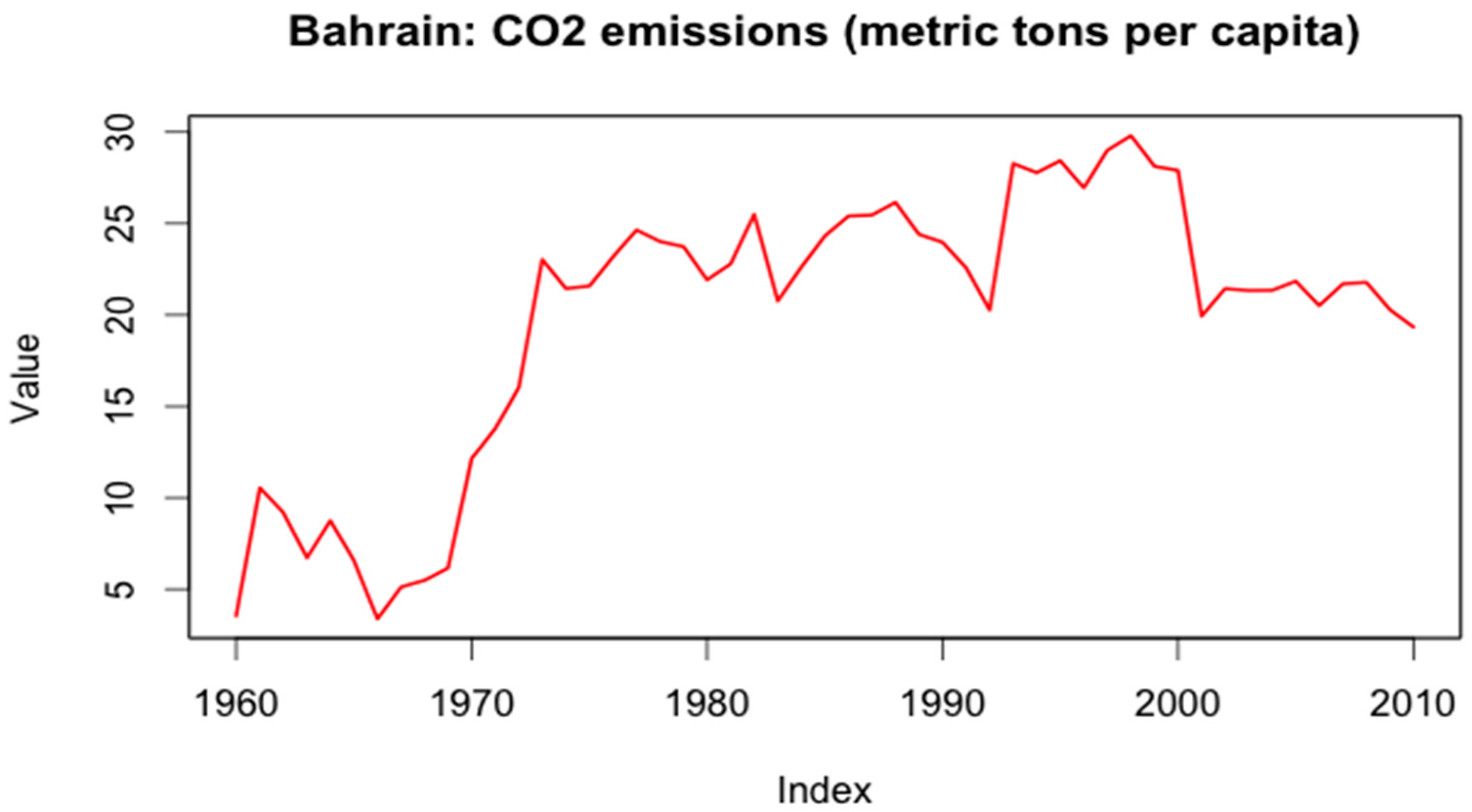
Figure 2 shows that CO2 emissions had an upward trend until 1998, after which it started to decrease sharply, and this decreasing trend continued until 2010. Over this 50-year period, some short-term reversals took place in 1963, 1966, 1974, 1983, and 1992, probably connected to the overall economic growth.
The graphical representation of data in Figure 2 indicates that this time series appears to be non-seasonal and can be described using an additive model. Thus, for a clearer view of the trend, we will use a smoothing method, by calculating the simple moving average of the time series. Figure 3 reflects the plot of the smoothed time series data of order 5.
The data smoothed with a simple moving average of order 5 shows that total carbon dioxide emissions for Bahrain measured in metric tons per capita increased from the level of 3.54 at the end of 1960 to a maximum level of 29.80 in 1998, and then decreased afterwards to about 20 at the end of 2001, reaching the level of 19.34 by the end of the analysis period. In addition, the decreasing trend started again with the global financial crisis, confirming the positive relationship between the economic growth and CO2 emissions attested in the academic literature.
4. Empirical Results
Similar to Silva (2013) [4] and Hassani et al. (2015) [11], we rely on the Root Mean Squared Error (RMSE) for evaluating and comparing the forecasting accuracies between the models. RMSE is the square root of the mean square error, and it has the advantage of being directly interpretable in terms of measurement units. In other words, RMSE takes the differences between each forecast and corresponding observed value, squares it, and averages it over the sample. Finally, the square root of the average is taken:
In Table 3, we present the model parameters for CO2 emissions in Bahrain for the training data set.
Table 4 reports the RMSE for out-of-sample forecasting results at a horizon of h = 18 steps ahead (covering the data test period, or 1994–2011) for the models described above, along with a “naive” forecasting model, which predicts a flat line equal to the last observation in the training set.
Results attest that NNAR is outperforming the rest of the models at h = 18 years ahead, while the ETS comes in second in terms of the lowest RMSE. On the other hand, it is obvious that Holt–Winters performs the worst, followed by the BATS/TBATS models.
In order to illustrate the effectiveness of the NNAR model in relation to the competing forecasts, Table 5 reports the Relative Root Mean Squared Error (RRMSE) results for the out-of-sample forecasts. For forecasting CO2 emissions in Bahrain, the NNAR forecast is found to be 35% better than the ETS forecast, 42% better than the naive model, 47% better than ARIMA, and 90% better than Holt–Winters for forecasting CO2 emissions in Bahrain.
Next, we test whether this difference between the forecasts of NNAR and the second-best alternative (i.e., ETS) is indeed statistically significant. Thus, the Hassani–Silva (HS) test is subsequently used (in R) to find significant differences between forecasts. Hassani and Silva (2016) [22] propose a non-parametric test founded upon the principles of the Kolmogorov–Smirnov (KS) test. The forecast errors from NNAR and ETS forecasting models are inputs into the two-sided HS test for determining the existence of a statistically significant difference in the distribution of forecasts errors from the two models. Here, the two-sided test statistic is significant at 1%, thus we can reject the null hypothesis and accept the alternate, which is that the forecast errors from NNAR and ETS do not share the same distribution. The HS test thus confirms that there is indeed a statistically significant difference between the distribution of forecast errors from NNAR and ETS at h = 18 steps ahead, thereby confirming that the NNAR forecasting technique provides superior forecasts in comparison to ETS.
Further, we make forecasts for carbon dioxide emissions in Bahrain in the 2012–2021 decade with the model that proved to be the best in terms of forecasting accuracy, i.e., NNAR.
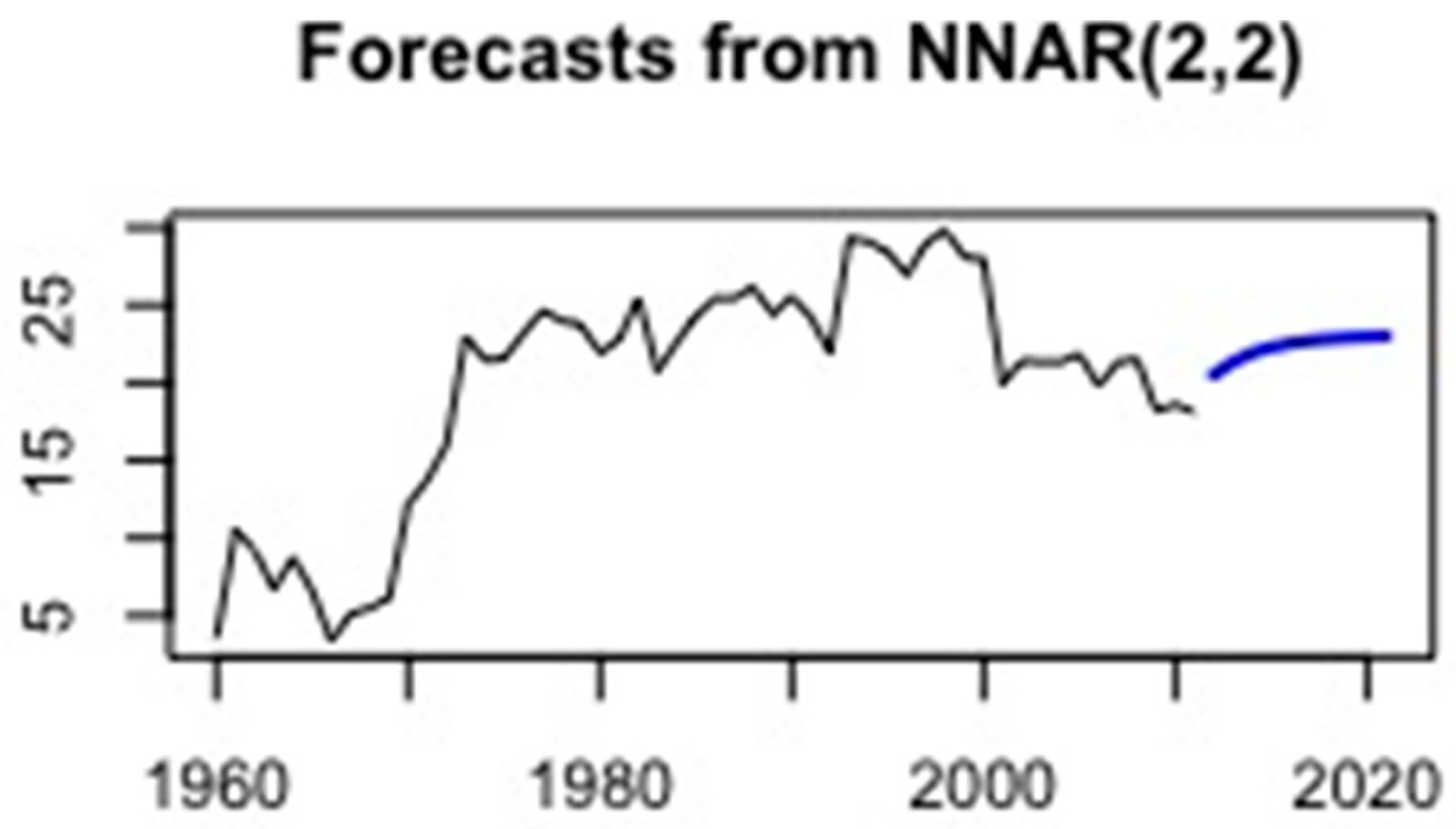
Table 6 gives the forecasted annual values for years 2012–2021. We should specify that the “nnetar” function in R will only provide point forecasts at this time, without giving the 80% and 95% prediction interval for the forecast, as is the case for other forecasting models implemented in R. Results indicate a reversal of the current decreasing trend for Bahrain’s CO2 emissions per capita in the next decade. Therefore, the model predicts that the country will see an increase of CO2 emissions, with a forecasted level of CO2 emissions in Bahrain for the year 2020 equal to 23.09 and, for 2021, equal to about 23.17.
Figure 4 reflects the predictions made by NNAR for 2012–2021 as a blue line. The reversal of the decreasing trend is again obvious.
Finally, we check the accuracy of the NNAR model by evaluating the in-sample forecast errors. We are interested in whether there is any autocorrelation left in the residuals, which would suggest that there is information that has not been accounted for in the proposed model. Thus, the Ljung-Box test is carried out in order to test whether there is significant evidence for non-zero correlations at lags 1–20. Here, the Ljung-Box test statistic is 18.129 with a p-value of 0.57, indicating that we have no autocorrelations in the in-sample forecast errors at lags 1–20.
5. Conclusions
The release of greenhouse gases (GHGs) in the atmosphere constitutes a major (and possibly most important) factor for the global warming phenomenon, and carbon dioxide (CO2) emissions account for 83 percent of total GHG emissions. For these considerations, an estimation of the evolution of CO2 emissions for the next decade is of paramount importance for current global political and economic agendas. This study focused on a single-country analysis (i.e., Bahrain) of future CO2 emissions through an automatic forecasting approach. Overall, this paper considered seven different forecasting models, which included the exponential smoothing state space model (ETS), the Holt–Winters Model, the BATS/TBATS model, ARIMA, the structural time series model (STS), the naive model, and the neural network time series forecasting method (NNAR). Based on the RMSE criterion, we find the NNAR model to provide the most accurate out-of-sample forecasts between the included models. Subsequently, our confidence in the NNAR is further increased by the HS test result, which confirms that the NNAR forecasting technique provides superior forecasts in comparison to the next best performing technique in terms of RMSE, i.e., the ETS technique. Finally, a battery of robustness checks confirmed the accuracy of the forecasting model that attests that Bahrain is not reducing its CO2 emissions and cannot meet its assumed obligation under the Doha amendment to the Kyoto protocol, which states that all countries should decrease their emissions by 18% by the year 2020 relative to their 1990 level. Thus, in the case of Bahrain, this would imply a maximum level of 20.96 metric tons per capita by the end of 2020, which the country seems to surpass according to our forecasted value of 23.09 metric tons per capita for 2020, which will further increase to 23.17 in 2021.
Future research could consider the role of other variables (such as population, per capita energy use, and energy mix) in predicting CO2 emissions and thus developing a multivariate model where CO2 emissions depend on these sub-variables, and this model can be further used for forecasting purposes.
Acknowledgments
This research was supported by CNCS-UEFISCDI, Project number IDEI 303, code PN-II-ID-PCE-2011-3-0593. I would like to thank an anonymous referee for many helpful comments.
Conflicts of Interest
The author declares no conflict of interest.
References
- European Environment Agency. Greenhouse Gas Emission Trends and Projections in Europe 2009; No 9/2009; European Environment Agency: Copenhagen, Denmark, 2009. [Google Scholar]
- The Economist. Available online: http://www.economist.com/blogs/graphicdetail/2011/12/daily-chart-6 (accessed on 8 September 2016).
- Meng, M.; Niu, D. Modeling CO2 emissions from fossil fuel combustion using the logistic equation. Energy 2011, 36, 3355–3359. [Google Scholar] [CrossRef]
- Silva, E.S. A combination forecast for energy-related CO2 emissions in the United States. Int. J. Energy Stat. 2013, 1, 269–279. [Google Scholar] [CrossRef]
- Wang, K.-M. The relationship between carbon dioxide emissions and economic growth: Quantile panel-type analysis. Qual. Quant. 2013, 47, 1337–1366. [Google Scholar] [CrossRef]
- Grubb, M.; Butler, L.; Feldman, O. Analysis of the Relationship between Growth in Carbon Dioxide Emissions and Growth in Income. 2006. Available online: www.econ.cam.ac.uk/rstaff/grubb/GA12.pdf (accessed on 5 September 2016).
- Hussain, M.; Javaid, M.; Drake, P.R. An econometric study of carbon dioxide (CO2) emissions, energy consumption, and economic growth of Pakistan. Int. J. Energy Sect. Manag. 2012, 6, 518–533. [Google Scholar] [CrossRef]
- Tudor, C. Changes in stock markets interdependencies as a result of the global financial crisis: Empirical investigation on the CEE region. Panoeconomicus 2011, 58, 525–543. [Google Scholar] [CrossRef]
- Koleini, A. Portfolio Diversification; Benefits of Investing in Carbon Markets from a New Zealand Investor Perspective. 2011. Available online: http://hdl.handle.net/10292/1346 (accessed on 5 September 2016).
- Chevallier, J. Energy Risk Management with Carbon Assets. 2009. Available online: hal.inria.fr/docs/00/chevallier_carbonrisk.pdf (accessed on 5 September 2016).
- Hassani, H.; Silva, E.S.; Gupta, R.; Segnon, M.K. Forecasting the price of gold. Appl. Econ. 2015, 47, 4141–4152. [Google Scholar] [CrossRef]
- Hyndman, R.J.; Athanasopoulos, G. Forecasting: Principles and Practice. Available online: www.OTexts.com/fpp (accessed on 5 September 2016).
- Hyndman, R.J.; Khandakar, Y. Automatic Time Series Forecasting: The forecast Package for R. J. Stat. Softw. 2008, 27, 1–22. [Google Scholar] [CrossRef]
- Hyndman, R.J.; Koehler, A.B.; Snyder, R.D.; Grose, S. A State Space Framework for Automatic Forecasting Using Exponential Smoothing Methods. Int. J. Forecast. 2002, 18, 439–454. [Google Scholar] [CrossRef]
- Chatfield, C. The Holt–Winters Forecasting Procedure. Appl. Stat. 1978, 27, 264–279. [Google Scholar] [CrossRef]
- Paraschiv, D.; Tudor, C.; Petrariu, R. The Textile Industry and Sustainable Development: A Holt–Winters Forecasting Investigation for the Eastern European Area. Sustainability 2015, 7, 1280–1291. [Google Scholar] [CrossRef]
- De Livera, A.M.; Hyndman, R.J.; Snyder, R.D. Forecasting time series with complex seasonal patterns using exponential smoothing. J. Am. Stat. Assoc. 2011, 106, 1513–1527. [Google Scholar] [CrossRef]
- Ripley, B.D. Time Series in R 1.5.0. R News 2011, 2, 2–7. [Google Scholar]
- R Manual, Fit Structural Time Series. Available online: https://stat.ethz.ch/R-manual/R-devel/library/stats/html/StructTS.html (accessed on 5 September 2016).
- Petris, G.; Petrone, S. State space models in R. J. Stat. Softw. 2011, 41, 1–25. [Google Scholar] [CrossRef]
- World Bank Database. Available online: http://data.worldbank.org/indicator/EN.ATM.CO2E.PC?locations=BH) (accessed on 5 September 2016).
- Hassani, H.; Silva, E.S. A Kolmogorov–Smirnov based test for comparing the predictive accuracy of two sets of forecasts. Econometrics 2016, 3, 590–609. [Google Scholar] [CrossRef] [Green Version]
Figure 1.
Total greenhouse gas emissions by sector in EU-27, 2008. Source of data: European Environment Agency [1].
Figure 1.
Total greenhouse gas emissions by sector in EU-27, 2008. Source of data: European Environment Agency [1].
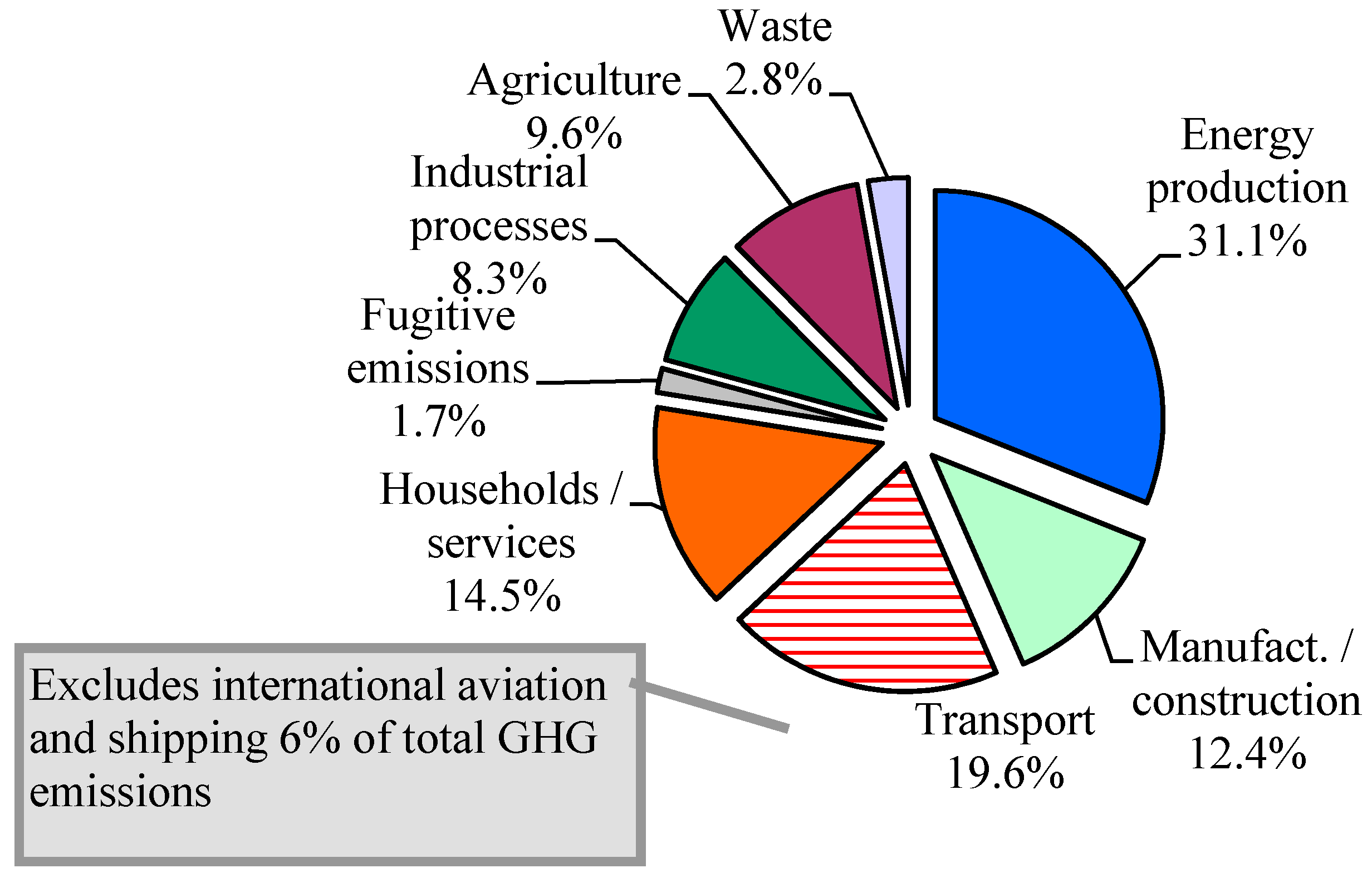
Figure 2.
Bahrain CO2 emissions over 1960–2011 (metric tons per capita).

Figure 3.
CO2 emissions in Bahrain smoothed with SMA of order 5.
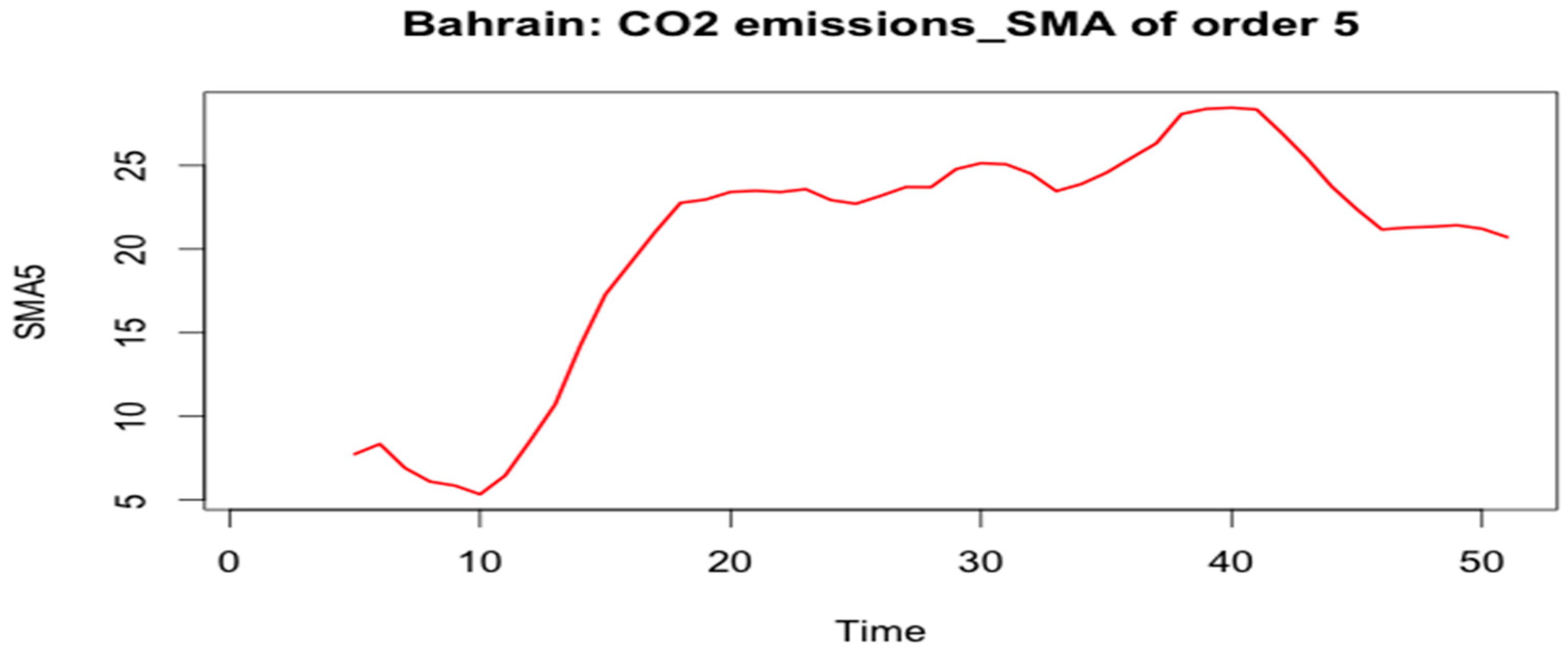
Figure 4.
Forecasts from NNAR (2,2).


| Country | Level | As of | 1 Year Chg | ~5 Year ago | ~10 Year ago | ~25 Year ago |
|---|---|---|---|---|---|---|
| USA | 5,433,056.54 kt | 2010 | 2.28% | 5,737,615.55 kt | 5,601,404.84 kt | 4,491,176.58 kt |
| China | 8,286,891.95 kt | 2010 | 7.73% | 6,414,463.08 kt | 3,487,566.36 kt | 2,068,969.07 kt |
| Japan | 1,170,715.42 kt | 2010 | 6.37% | 1,231,301.59 kt | 1,202,266.29 kt | 915,327.20 kt |
| Germany | 745,383.76 kt | 2010 | 1.79% | 808,859.53 kt | 853,662.93 kt | n.a. |
| France | 361,272.84 kt | 2010 | 1.22% | 382,581.78 kt | 385,827.07 kt | 385,614.39 kt |
| Brazil | 419,754.16 kt | 2010 | 14.33% | 347,668.27 kt | 337,433.67 kt | 198,883.41 kt |
| UK | 493,504.86 kt | 2010 | 3.87% | 542,041.27 kt | 550,552.38 kt | 568,777.37 kt |
| Italy | 406,307.27 kt | 2010 | 1.17% | 469,346.66 kt | 450,347.94 kt | 366,454.31 kt |
| Russia | 1,740,776.24 kt | 2010 | 10.57% | 1,669,618.10 kt | 1,558,012.96 kt | n.a. |
| India | 2,008,822.94 kt | 2010 | 1.34% | 1,504,364.75 kt | 1,203,843.10 kt | 525,862.47 kt |
| Canada | 499,137.37 kt | 2010 | −2.88% | 550,233.35 kt | 525,690.12 kt | 387,220.53 kt |
| Australia | 373,080.58 kt | 2010 | −5.57% | 371,214.08 kt | 324,859.53 kt | 239,964.81 kt |
| Spain | 269,674.85 kt | 2010 | −6.44% | 350,037.15 kt | 297,830.07 kt | 190,467.65 kt |
| Mexico | 443,674.00 kt | 2010 | −0.57% | 441,796.49 kt | 394,800.22 kt | 294,559.11 kt |
| South Korea | 567,567.26 kt | 2010 | 11.42% | 470,806.13 kt | 450,193.92 kt | 182,451.58 kt |
| Indonesia | 433,989.45 kt | 2010 | −4.22% | 345,119.71 kt | 294,907.47 kt | 121,740.73 kt |
| Turkey | 298,002.42 kt | 2010 | 7.25% | 261,570.78 kt | 194,538.02 kt | 116,881.96 kt |
| Saudi Arabia | 464,480.55 kt | 2010 | 7.76% | 432,739.00 kt | 297,214.02 kt | 204,878.96 kt |
| Argentina | 180,511.74 kt | 2010 | 0.49% | 174,237.51 kt | 132,631.72 kt | 104,212.47 kt |
| South Africa | 460,124.16 kt | 2010 | −8.69% | 424,843.95 kt | 362,743.31 kt | 330,855.08 kt |
| Country | Level | Units | As of | 1 Year Chg | ~5 Year ago | ~10 Year ago | ~25 Year ago |
|---|---|---|---|---|---|---|---|
| Algeria | 123,475.22 | kt | 2010 | −0.89% | 103,963.12 | 84,293.33 | 76,277.27 |
| Bahrain | 24,202.20 | kt | 2010 | 0.14% | 19,497.44 | 13,927.27 | 11,012.00 |
| Djibouti | 539.05 | kt | 2010 | 1.38% | 487.71 | 385.04 | 385.04 |
| Egypt | 204,776.28 | kt | 2010 | 3.49% | 178,615.90 | 125,451.74 | 74,564.78 |
| Iran | 571,611.96 | kt | 2010 | −1.02% | 509,889.02 | 398,826.59 | 148,568.51 |
| Iraq | 114,667.09 | kt | 2010 | 7.52% | 99,544.38 | 85,342.09 | 47,751.67 |
| Israel | 70,655.76 | kt | 2010 | 5.41% | 65,976.66 | 65,749.31 | 26,626.09 |
| Jordan | 20,821.23 | kt | 2010 | −2.04% | 20,733.22 | 16,002.79 | 9281.18 |
| Kuwait | 93,695.52 | kt | 2010 | 14.45% | 73,769.04 | 55,122.34 | 35,320.54 |
| Lebanon | 20,403.19 | kt | 2010 | −2.45% | 14,499.32 | 16,208.14 | 7759.37 |
| Libya | 59,035.03 | kt | 2010 | −12.77% | 53,787.56 | 48,100.04 | 34,059.10 |
| Malta | 2588.90 | kt | 2010 | 3.67% | 2574.23 | 2486.23 | 1485.13 |
| Morocco | 50,608.27 | kt | 2010 | 2.15% | 47,425.31 | 37,715.10 | 18,881.38 |
| Oman | 57,201.53 | kt | 2010 | 42.07% | 39,603.60 | 20,285.84 | 9875.23 |
| Qatar | 70,531.08 | kt | 2010 | 6.67% | 56,735.82 | 30,362.76 | 13,296.54 |
| Saudi Arabia | 464,480.55 | kt | 2010 | 7.76% | 432,739.00 | 297,214.02 | 204,878.96 |
| Syria | 61,858.62 | kt | 2010 | −0.41% | 53,589.54 | 48,785.77 | 31,352.85 |
| Tunisia | 25,878.02 | kt | 2010 | 4.32% | 23,127.77 | 20,817.56 | 12,064.43 |
| UAE | 167,596.57 | kt | 2010 | 3.07% | 123,874.93 | 101,414.55 | 47,234.63 |
| Yemen | 21,851.65 | kt | 2010 | −5.23% | 20,795.56 | 16,252.14 | 8269.08 |
| Model | Parameters |
|---|---|
| Neural Network Model (NNAR) (p,k) | (2,2) |
| ETS (A,N,N) (α) | 0.8742 |
| ARIMA (p,d,q) | (3,1,0) |
| Structural Time Series Model (STS) | Level: 4.6409 |
| Slope: 0.02376 | |
| Epsilon: 1.2511 | |
| TBATS | (1, {0,0}, 0.922, -) |
| Holt–Winters (α,β,γ) | (0.8905, 0.3669, false) |
Note: p is the number of non-seasonal lags used as inputs, and k (size) is the number of nodes in the hidden layer; the automatically selected ETS model is of the form (A,N,N), so there is no trend nor any seasonal component in the data; ARIMA parameters are automatically found by function auto.arima in R (the number of differences d is determined using repeated KPSS tests, while the values of p and q are then chosen by minimizing the AICC after differencing the data d times); STS is a local linear trend model as implemented in function StructTS in R, and parameters are estimations of variances: level is the variance of the level disturbances, slope is the variance of the slope disturbances, and epsilon is the variance of the observation disturbances; TBATS function in R fits a TBATS model applied to the training data, as described by De Livera, Hyndman and Snyder (2011) [17].
| Forecasting Model (Train on First 33 Observations, Test on Last 18 Observations) | RMSE (h = 18) |
|---|---|
| Neural Network Model (NNAR) | 3.98 |
| ETS | 6.15 |
| Naive Model | 6.85 |
| ARIMA | 7.48 |
| Structural Time Series Model (STS) | 12.91 |
| BATS/TBATS | 20.16 |
| Holt–Winters | 39.59 |
| Forecasting Model | RRMSE |
|---|---|
| NNAR/ETS | 0.65 * |
| NNAR/Naive Model | 0.58 |
| NNAR/ARIMA | 0.53 |
| NNAR/STS | 0.31 |
| NNAR/TBATS | 0.20 |
| NNAR/Holt–Winters | 0.10 |
Note: * indicates there exists a statistically significant difference between the distribution of forecast errors from the best and second best performing models based on the two-sided HS test at a 1% significance level (the computed HS test equals 0.61 with a p-value of 0.0018).
Table 6.
Carbon dioxide emissions in Bahrain, metric tons per capita (forecasted values for 2012–2021).
| Year | Point Forecast |
|---|---|
| 2012 | 20.36337 |
| 2013 | 21.03039 |
| 2014 | 21.65644 |
| 2015 | 22.10237 |
| 2016 | 22.43456 |
| 2017 | 22.68002 |
| 2018 | 22.86189 |
| 2019 | 22.99681 |
| 2020 | 23.09705 |
| 2021 | 23.17162 |
© 2016 by the author; licensee MDPI, Basel, Switzerland. This article is an open access article distributed under the terms and conditions of the Creative Commons Attribution (CC-BY) license (http://creativecommons.org/licenses/by/4.0/).
Share and Cite
MDPI and ACS Style
Tudor, C. Predicting the Evolution of CO2 Emissions in Bahrain with Automated Forecasting Methods. Sustainability 2016, 8, 923. https://doi.org/10.3390/su8090923
AMA Style
Tudor C. Predicting the Evolution of CO2 Emissions in Bahrain with Automated Forecasting Methods. Sustainability. 2016; 8(9):923. https://doi.org/10.3390/su8090923
Chicago/Turabian StyleTudor, Cristiana. 2016. "Predicting the Evolution of CO2 Emissions in Bahrain with Automated Forecasting Methods" Sustainability 8, no. 9: 923. https://doi.org/10.3390/su8090923
Note that from the first issue of 2016, this journal uses article numbers instead of page numbers. See further details here.