Exploring Land Use and Land Cover of Geotagged Social-Sensing Images Using Naive Bayes Classifier

Abstract

Online social media crowdsourced photos contain a vast amount of visual information about the physical properties and characteristics of the earth’s surface. Flickr is an important online social media platform for users seeking this information. Each day, users generate crowdsourced geotagged digital imagery containing an immense amount of information. In this paper, geotagged Flickr images are used for automatic extraction of low-level land use/land cover (LULC) features. The proposed method uses a naive Bayes classifier with color, shape, and color index descriptors. The classified images are mapped using a majority filtering approach. The classifier performance in overall accuracy, kappa coefficient, precision, recall, and f-measure was 87.94%, 82.89%, 88.20%, 87.90%, and 88%, respectively. Labeled-crowdsourced images were filtered into a spatial tile of a 30 m × 30 m resolution using the majority voting method to reduce geolocation uncertainty from the crowdsourced data. These tile datasets were used as training and validation samples to classify Landsat TM5 images. The supervised maximum likelihood method was used for the LULC classification. The results show that the geotagged Flickr images can classify LULC types with reasonable accuracy and that the proposed approach improves LULC classification efficiency if a sufficient spatial distribution of crowdsourced data exists.

1. Introduction

The availability of volunteered geographic information (VGI) from social media has exponentially increased over the last few years [1]. Since the emergence of Web 2.0, an increasing number of users have uploaded georeferenced photographs on social media websites, such as Flickr, Picasa, Webshoot, Panoramio, and Geograph [2,3,4,5,6]. Owing to advancements in camera and mobile technology, social media photos contain a vast amount of information, ranging from non-spatial information, such as tags, titles, and descriptions, to spatial and temporal information, such as the locations and times in which the photos were taken. Georeferenced Flickr images [6,7,8], for example, can be used in various applications, such as navigation, natural disaster response (e.g., wildfires, earthquakes, and floods), disease outbreak response, crisis management, and other emergency responses [9,10,11]. Collecting, searching, and analyzing these types of photo repositories can provide information of social and practical importance.

Land cover maps of the earth represent both human-made and natural characteristics of the earth’s surface. Various scientific land cover products, covering various spatial and temporal resolutions, have been created using remotely sensed imagery, such as Moderate Resolution Imaging Spectroradiometer (MODIS), Global Land Cover SHARE (GLC-SHARE), Global Land Cover 2000 (GLC2000), International Geosphere-Biosphere Programme (IGBP), and GlobeCover [12]. The classification accuracies and validations of these regional products are a great concern for the scientific community because of the lack of training and validation data. Consequently, geotagged images have become increasingly prevalent via social media, which can be used as supporting data for scientific analysis [13].

Performing feature extraction of crowdsourced information is now possible owing to the rapid development of information technology. Several researchers have demonstrated that social-sensing image features extracted from photographs (such as on Flickr) include visual descriptors of color, edges, and color indices that can be used for land cover mapping [14,15].

The critical issue with VGI is the need for a means to extract quality information from crowdsourced data and determining its reliability using other LULC products [13]. To create meaningful information from VGI, a highly accurate scientific experiment is required that includes sampling, training, validation, and suitable classification algorithms. Some studies have reviewed these crowdsourced geographic information terms; nevertheless, few examples exist of these techniques being collated to land cover classification [5].

With the above considerations, this paper presents the exploration of crowdsourced LULC types that share certain image characteristics with the major LULC types, including urban areas, forest, agricultural areas, water bodies, and grassland. The integration of crowdsourced LULC maps can be linked to satellite remote-sensing data for creating LULC products [16]. The technical challenge is developing a method to convert visual features from crowdsourced data (e.g., Flickr images) into LULC types by acquiring a sufficient amount of quality references for using remote sensing applications.

The objective of this study is thus to automatically extract visual LULC descriptions from online photos and to estimate the probability distributions over LULC types for a particular area of interest. We herein demonstrate the: (1) automatic extraction of geotagged social-sensing images for visual LULC descriptions from Flickr; (2) classification of Flickr images into major LULC types (agricultural, forest, grassland, urban structures, and water bodies) using a naive Bayes classifier model; and (3) use of majority voting to reduce the uncertainty inherent in estimating LULC types from crowdsourced images.

2. Study Area and Dataset

2.1. Crowdsourced Data

For the study dataset, we acquired and downloaded more than 1,000,000 geotagged images from Flickr obtained in Sapporo City, Japan, using the Flickr Application Programming Interface (API). Sapporo City covers a total area of 1121 km². Flickr contains a large volume of images distributed over Sapporo. Figure 1 shows the Flickr image density per square kilometer. Flickr metadata for each image contain useful information about it, including the title, description, tags, authors, GPS location, and date and time of when the image was obtained and uploaded. From the available dataset, we selected all images obtained between 1 January and 31 December 2009. The Flickr metadata, such as tags, date taken, image location, and image characteristics were used to produce a filtered list of images.

2.2. Landsat TM5 Data

In this study, we chose Landsat TM5 imagery for integration with crowdsourced data. A significant data source, Landsat TM5 imagery, is freely available and one of the most commonly used satellite imagery repositories for regional and global LULC applications. The Landsat TM5 image used in this study was selected from the Land Processes Distributed Active Archive Center (LPDAAC) [17] and scene path/row 107/030. The thermal band (band 6) was excluded from the analysis. The image is dated 28 May 2009 and has a resolution of 30 m × 30 m in the WGS84 geographic coordinate reference system (World Geodetic System 1984) covering Sapporo City. The image was converted to top-of-atmosphere (TOA) reflectance and then atmospherically corrected using a dark pixel subtraction method.

3. Methodology

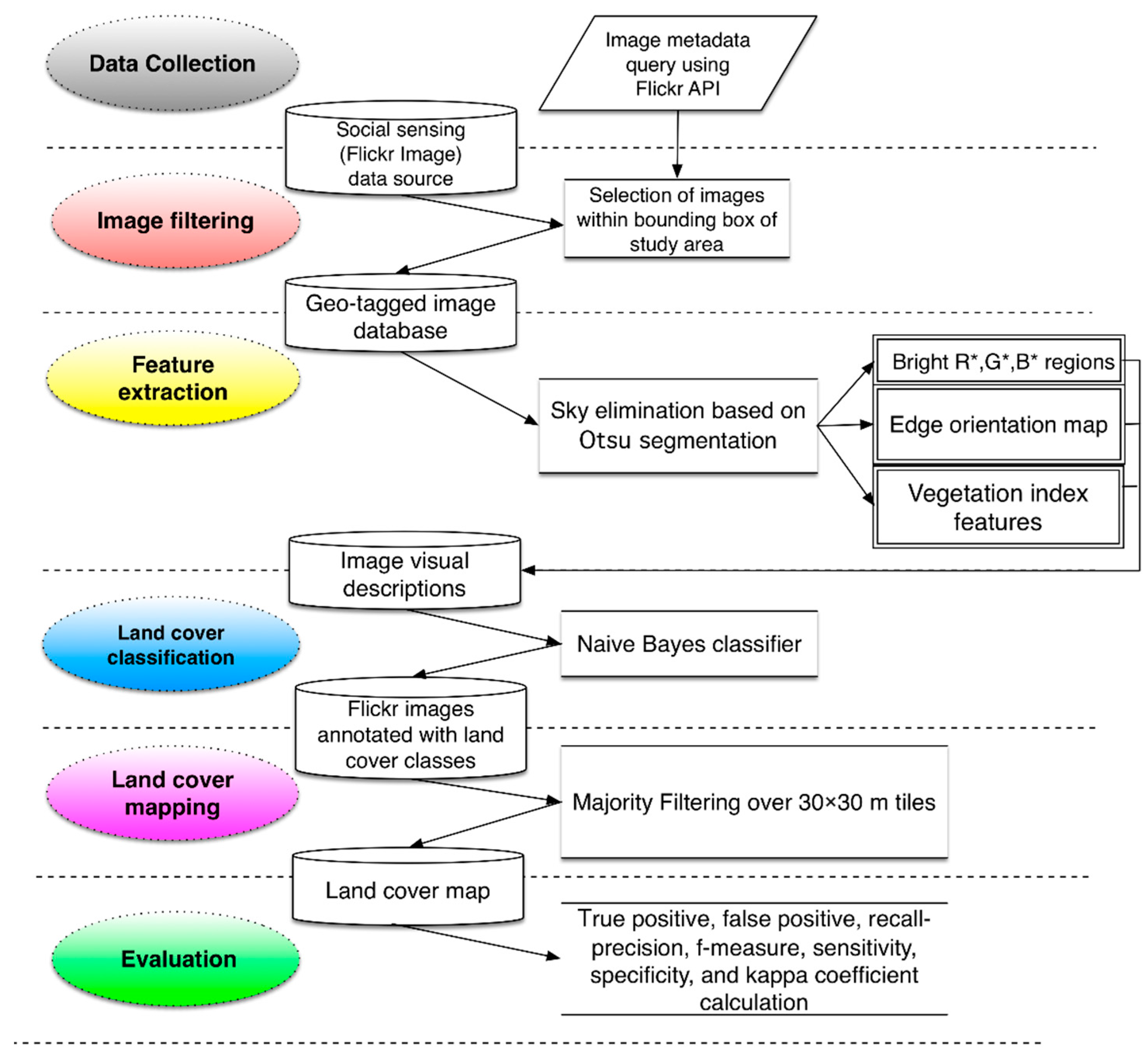
The aim of this research was to extract a precise and accurate LULC type for each geotagged image that can be used for practical LULC mapping. The image-based results are then used to classify the LULC of each tile in the map. Figure 2 presents a schematic of our approach. We first perform low-level image feature extraction to characterize the visual appearance of an image. These features include color, edge content, and color index descriptors. Low-level feature extraction is followed by classification. Then, the image-based results are mapped to geospatial locations. In this section, we provide details of our pipeline, including low-level feature extraction, naive Bayes classification, and majority voting for tiled (30 m × 30 m Landsat-scale pixel) LULC mapping.

3.1. Automatic Low-Level Image Feature Extraction from Flickr Data

Image analysis is a mathematical process that extracts, characterizes, and interprets information contained in the digital pixel elements of photographic images. Examples include finding shapes, counting objects, identifying colors, and measuring object properties [18,19]. In this study, we develop visual feature extractors for land cover extraction. We use color histograms to summarize the distribution of colors in an image, gradient orientation maps to indicate shape [14], and color indices characterize vegetation [20]. Finally, we combine these image features with statistical analysis in the form of a Bayes classifier [19,21].

In the first step, the image is segmented to remove prospective sky regions. Then, the low-level color, edge, and vegetation features are calculated over the probable non-sky regions. In the next step, we build a naive Bayes classifier to perform maximum likelihood estimation of the LULC type for a given image. We use a majority filtering method to obtain the most likely LULC category for each tile on the map.

3.1.1. Image Segmentation

Image segmentation is the process of sub-dividing an image into regions, parts, or objects, where each part or object is homogeneous, so that each of the resulting regions in the image can be separately analyzed [22,23]. Background or foreground segmentation can use different techniques, such as image-based thresholding, edge-based segmentation, and color-based segmentation. The main purpose of this step is to automatically separate the subject from the sky and other irrelevant features [22].

Accordingly, we employ Otsu thresholding to separate the foreground and background into two non-overlapping binary sets of color pixels. The Otsu method calculates a probability distribution over pixel intensities and then finds the optimal threshold (T) separating the two assumed intensity classes by minimizing the variance within each class and maximizing the separation of the two classes [24,25,26,27]. The result is a binary mask, F, indicating the two classes. The connected components of this binary mask are considered foreground segments.

$$\mathrm{F}\left(\mathrm{x},\mathrm{y}\right)=\{\begin{array}{l}1\mathrm{if}\mathrm{I}\left(\mathrm{x},\mathrm{y}\right)<\mathrm{T},\\ 0\mathrm{otherwise}.\end{array}$$

(1)

where T is the threshold and I(x, y) is the intensity of the input pixel at location (x, y).

Pixels in the image with intensities that are less than T are classified as foreground, whereas image pixels with intensities that are greater than or equal to T are classified as sky/background according to Equation (1) [28]. RGB channel features are obtained by multiplying the original RGB image with the binary foreground image. However, face images are filtered out before further feature extraction using a face detection approach [14]. We additionally consider animals or other objects as noise or misclassified images using the majority voting method described in Section 3.5.

3.1.2. Feature Extraction

Content-based image retrieval (CBIR) is the application of computer vision techniques to image retrieval problems [29]. We adapt some of the features typically used in CBIR to perform automatic land cover classification. We automatically compute image features from a large database (Flickr). We extract RGB histograms, edge orientation maps, and vegetation indices (color indices) as our features.

(a)

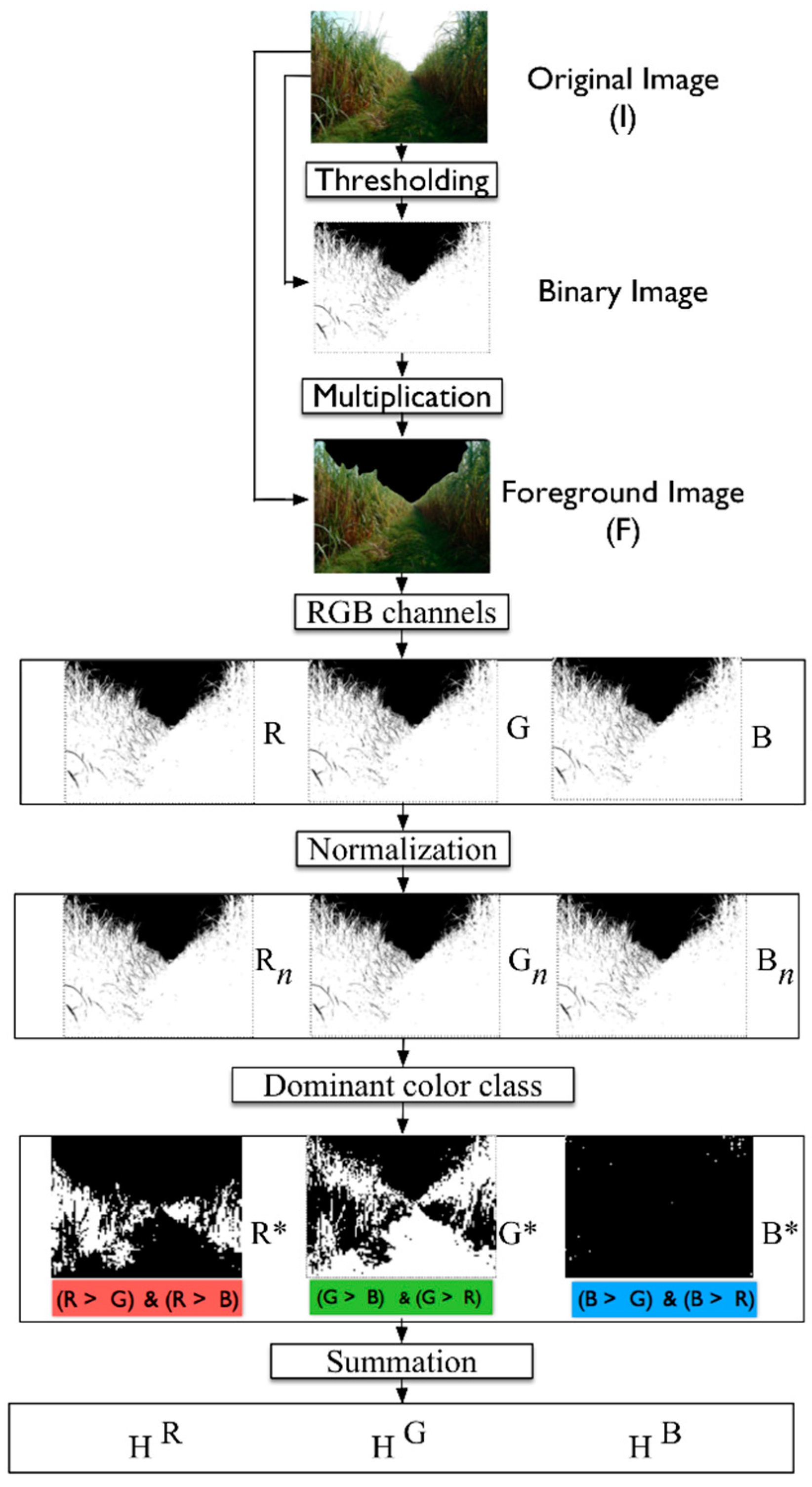
RGB histogram: Color features are among the most widely used visual features in CBIR. See Figure 3 for a diagram that summarizes our image segmentation and RGB feature extraction approach. We assume that the input is a three-channel RGB image with possible sky regions segmented as background. It is assumed that the remaining pixels are foreground. Because color is more important than intensity, we normalize the RGB image, as follows, to reduce dependency on the illumination conditions (Equation (2)) [20,30]. See Figure 3 for an example of RGB feature extraction.

$$\begin{gathered} {\mathrm{R}}_{\mathrm{n}}\left(\mathrm{x},\mathrm{y}\right)=\frac{\mathrm{R}\left(\mathrm{x},\mathrm{y}\right)}{\mathrm{R}\left(\mathrm{x},\mathrm{y}\right)+\mathrm{G}\left(\mathrm{x},\mathrm{y}\right)+\mathrm{B}\left(\mathrm{x},\mathrm{y}\right)}, \\ {\mathrm{G}}_{\mathrm{n}}\left(\mathrm{x},\mathrm{y}\right)=\frac{\mathrm{G}\left(\mathrm{x},\mathrm{y}\right)}{\mathrm{R}\left(\mathrm{x},\mathrm{y}\right)+\mathrm{G}\left(\mathrm{x},\mathrm{y}\right)+\mathrm{B}\left(\mathrm{x},\mathrm{y}\right)}, \\ {\mathrm{B}}_{\mathrm{n}}\left(\mathrm{x},\mathrm{y}\right)=\frac{\mathrm{B}\left(\mathrm{x},\mathrm{y}\right)}{\mathrm{R}\left(\mathrm{x},\mathrm{y}\right)+\mathrm{G}\left(\mathrm{x},\mathrm{y}\right)+\mathrm{B}\left(\mathrm{x},\mathrm{y}\right)}. \end{gathered}$$

(2)

Each pixel is then classified according to the dominant color following the scheme of Equation (3).

$$\begin{gathered} {\mathrm{R}}^{*}\left(\mathrm{x},\mathrm{y}\right)=\{\begin{array}{l}1\mathrm{if}{\mathrm{R}}_{\mathrm{n}}\left(\mathrm{x},\mathrm{y}\right)>{\mathrm{B}}_{\mathrm{n}}\left(\mathrm{x},\mathrm{y}\right)\mathrm{and}{\mathrm{R}}_{\mathrm{n}}\left(\mathrm{x},\mathrm{y}\right)>{\mathrm{G}}_{\mathrm{n}}\left(\mathrm{x},\mathrm{y}\right),\\ 0\mathrm{otherwise}\end{array} \\ {\mathrm{G}}^{*}\left(\mathrm{x},\mathrm{y}\right)=\{\begin{array}{l}1\mathrm{if}{\mathrm{G}}_{\mathrm{n}}\left(\mathrm{x},\mathrm{y}\right)>{\mathrm{B}}_{\mathrm{n}}\left(\mathrm{x},\mathrm{y}\right)\mathrm{and}{\mathrm{G}}_{\mathrm{n}}\left(\mathrm{x},\mathrm{y}\right)>{\mathrm{R}}_{\mathrm{n}}\left(\mathrm{x},\mathrm{y}\right),\\ 0\mathrm{otherwise}\end{array} \\ {\mathrm{B}}^{*}\left(\mathrm{x},\mathrm{y}\right)=\{\begin{array}{l}1\mathrm{if}{\mathrm{B}}_{\mathrm{n}}\left(\mathrm{x},\mathrm{y}\right)>{\mathrm{R}}_{\mathrm{n}}\left(\mathrm{x},\mathrm{y}\right)\mathrm{and}{\mathrm{B}}_{\mathrm{n}}\left(\mathrm{x},\mathrm{y}\right)>{\mathrm{G}}_{\mathrm{n}}\left(\mathrm{x},\mathrm{y}\right),\\ 0\mathrm{otherwise}\end{array} \end{gathered}$$

(3)

The resulting binary images (R*, G*, B*) indicate the locations of primary red, green, and blue pixels in the original image. The final RGB histogram features used as input for the Bayes classifier are simply the number of pixels classified as red, green, and blue, respectively. In sum, we compute the histogram (${\mathrm{H}}^{\mathrm{R}}$, ${\mathrm{H}}^{\mathrm{B}}\mathrm{and}{\mathrm{H}}^{\mathrm{G}}$) according to Equation (4).

$${\mathrm{H}}^{\mathrm{R}}={\displaystyle \sum }_{\mathrm{x},\mathrm{y}}{\mathrm{R}}^{*}\left(\mathrm{x},\mathrm{y}\right);{\mathrm{H}}^{\mathrm{G}}={\displaystyle \sum }_{\mathrm{x},\mathrm{y}}{\mathrm{G}}^{*}\left(\mathrm{x},\mathrm{y}\right);{\mathrm{H}}^{\mathrm{B}}={\displaystyle \sum }_{\mathrm{x},\mathrm{y}}{\mathrm{B}}^{*}\left(\mathrm{x},\mathrm{y}\right).$$

(4)

(b)

Edge orientation: No universal definition of shape exists in an RGB image. However, shape impressions can be extracted by color, intensity patterns, or texture, while a geometric representation can be derived from these impressions. Image edges are characterized by location, magnitude, and orientation [31,32]. Edge orientation is especially useful in distinguishing urban or other developed scenes from undeveloped scenes based on the principle that images of developed scenes will have higher proportions of horizontal and vertical edges than images of undeveloped scenes.

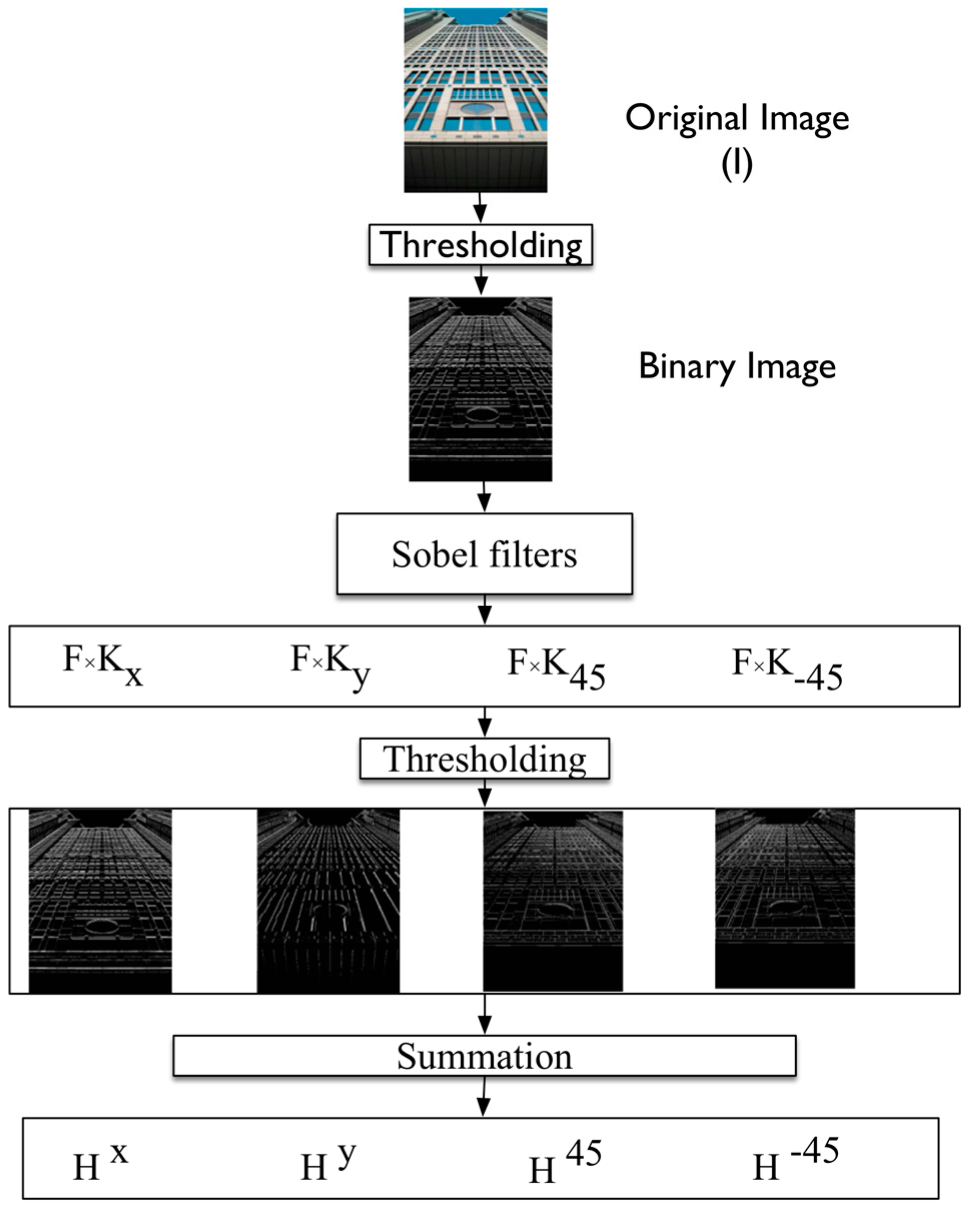
We thus extract edge histogram descriptors to identify the distribution of edges at different orientations across the image. See Figure 4 for a schematic of our edge orientation histogram extraction approach. We use F, the binary result of Otsu segmentation from the previous step. We apply four 3 × 3 Sobel edge kernels, which are tuned to detect edges in the horizontal (${\mathrm{K}}_{\mathrm{x}}$), vertical (${\mathrm{K}}_{\mathrm{y}}$), 45° diagonal (${\mathrm{K}}_{45}$), and −45° diagonal (${\mathrm{K}}_{-45}$) directions as follows:

$${\mathrm{K}}_{\mathrm{x}}=\left(\begin{array}{ccc}-1& 0& 1\\ -2& 0& 2\\ -1& 0& 1\end{array}\right),{\mathrm{K}}_{\mathrm{y}}=\left(\begin{array}{ccc}-1& -2& -1\\ 0& 0& 0\\ 1& 2& 1\end{array}\right),{\mathrm{K}}_{45}=\left(\begin{array}{ccc}-2& -1& 0\\ -1& 0& 1\\ 0& 1& 2\end{array}\right),{\mathrm{K}}_{-45}=\left(\begin{array}{ccc}0& 1& 2\\ -1& 0& 1\\ -2& -1& 0\end{array}\right)$$

The filter response magnitude indicates the intensity of the gradient at a given pixel in a particular direction [24]. We formulate the magnitude threshold of the outputs F × K_x, F × K_y, F × K₄₅ and F × K₋₄₅ of these filters to convert each edge magnitude image into a binary image. We classify each pixel with a gradient magnitude above the threshold as a possible horizontal, vertical, diagonal up, or diagonal down edge. The binary-oriented edge images are then summed, yielding four features (H^x, H^y, H⁴⁵, and H⁻⁴⁵).

(c)

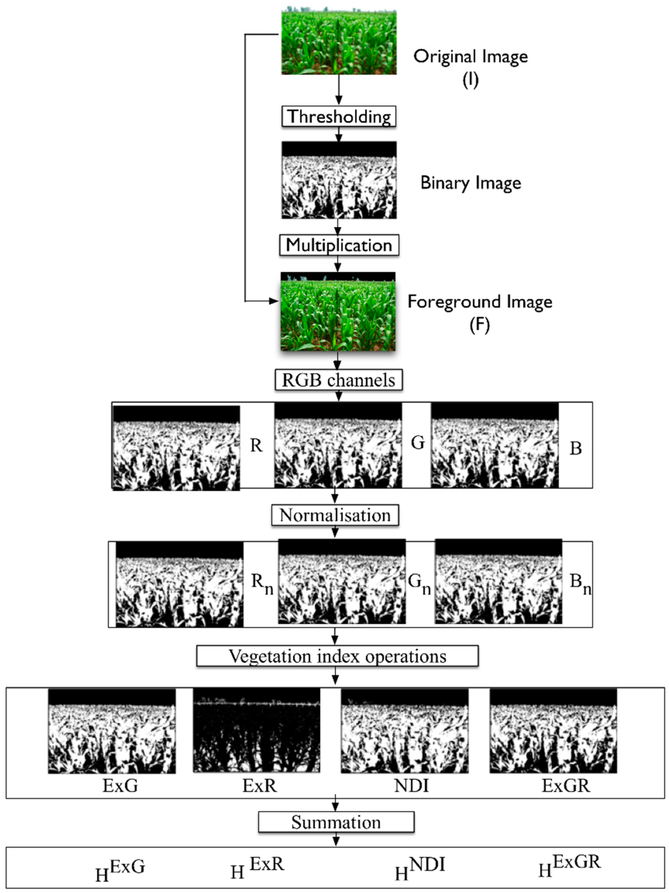
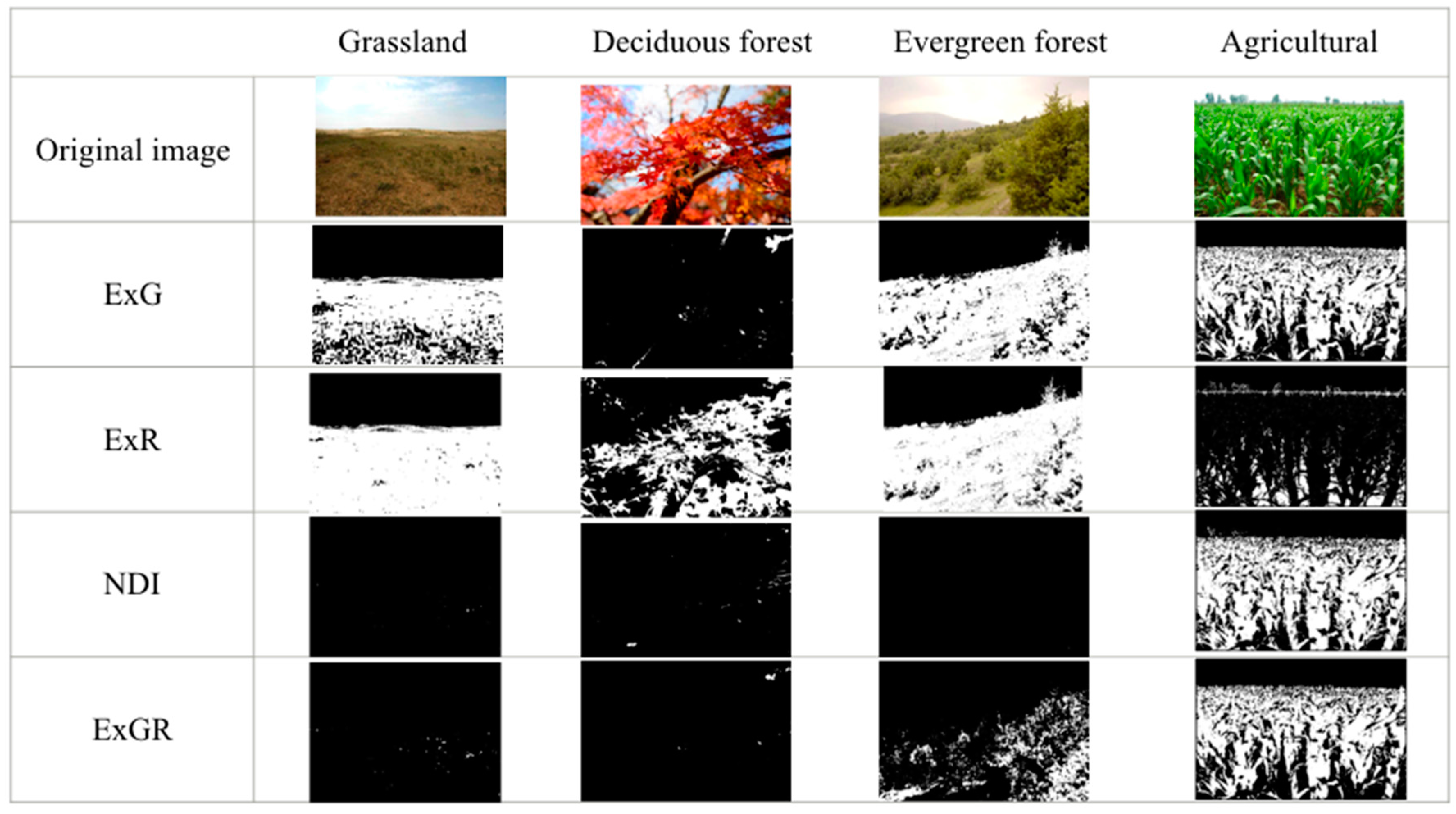
Vegetation Index (VI): Flickr images are normally three-layer images consisting of red, green and blue color planes, each representing the intensity of light in a range of color in the visible spectrum. Our vegetation descriptors (features) characterize vegetation content through the use of several VIs, particularly, excess green (ExG), excess red (ExR), normalized difference index (NDI), and difference of excess green and excess red (ExGR) [20], which are applied to each pixel’s chromatic coordinate. See Figure 5 for a schematic of the vegetation index histogram extraction approach.

The main aim of this approach is to extract prospective vegetation locations from the input image through analysis of the RGB channels (chromatic coordinates) of every pixel.

Table 1. Vegetation index operations.

Indices	Equation
ExG	2${\mathrm{G}}_{\mathrm{n}}\left(\mathrm{x},\mathrm{y}\right)-{\mathrm{R}}_{\mathrm{n}}\left(\mathrm{x},\mathrm{y}\right)-{\mathrm{B}}_{\mathrm{n}}\left(\mathrm{x},\mathrm{y}\right)$
ExR	1.4${\mathrm{R}}_{\mathrm{n}}\left(\mathrm{x},\mathrm{y}\right)-{\mathrm{G}}_{\mathrm{n}}\left(\mathrm{x},\mathrm{y}\right)$
NDI	${\mathrm{G}}_{\mathrm{n}}\left(\mathrm{x},\mathrm{y}\right)-{\mathrm{R}}_{\mathrm{n}}\left(\mathrm{x},\mathrm{y}\right)/{\mathrm{G}}_{\mathrm{n}}\left(\mathrm{x},\mathrm{y}\right)+{\mathrm{R}}_{\mathrm{n}}\left(\mathrm{x},\mathrm{y}\right)$
ExGR	ExG − ExR

shows the four vegetation index operations derived from the ${\mathrm{R}}_{\mathrm{n}}\left(\mathrm{x},\mathrm{y}\right)$, ${\mathrm{G}}_{\mathrm{n}}\left(\mathrm{x},\mathrm{y}\right),$ and ${\mathrm{B}}_{\mathrm{n}}\left(\mathrm{x},\mathrm{y}\right)$ planes. They extracted greenness information and differentiated between vegetation, soil, and residues. The advantage of using VIs is that they are renowned as being accurate at representing characteristics such as plant greenness [23].

The vegetation indices are summarized by binarization and then summed to obtain four features (H^NDI, H^ExG, H^ExR, and H^ExGR). ExG [33,34,35,36,37] selects plant regions of interest. ExR is related to the redness of the soil and residue. We use ExR to separate grassland from other types of vegetation, such as agriculture and forest. NDI is useful for separating plants from soil and residue in the background. Nonetheless, we determined that illumination has a significant impact on the usefulness of NDI. Meyer and Neto [20] used ExGR to extract dominantly green regions from images. Each of the four VI images is binarized using Otsu thresholding prior to summation to obtain H^NDI, H^ExG, H^ExR, and H^ExGR.

After computing all images through different feature extraction techniques, 11 feature histograms are obtained from each image: H^R, H^G, H^B, H^x, H^y, H⁴⁵, H⁻⁴⁵, H^NDI, H^ExG, H^ExR, and H^ExGR. These features are the input parameters obtained from each image to classify the LULC into a class. They are then used for further LULC classification.

3.2. Crowdsourced LULC Classification

We use the principle of probabilistic minimum risk classification to place each input image in a category. Each image is represented by the previously described vector of low-level features extracted from the image based on pixel-level properties. The simple but effective naive Bayes classifier is used because it is fast to train and not sensitive to irrelevant features [31].

We begin with the Bayes rule to compute the posterior probability, $\mathrm{P}(\mathrm{c}|\stackrel{\rightharpoonup }{\mathrm{d}}),$ of category c. Data $\stackrel{\rightharpoonup }{\mathrm{d}}$ are proportional to the product of prior probability P(c) and class-conditional probability $\mathrm{P}(\stackrel{\rightharpoonup }{\mathrm{d}}|\mathrm{c})$. The latter is from data given by the LULC class of the image according to Equation (5).

$$\mathrm{P}(\mathrm{c}|\stackrel{\rightharpoonup }{\mathrm{d}})=\mathrm{P}(\mathrm{c})\frac{\mathrm{P}(\stackrel{\rightharpoonup }{\mathrm{d}}|\mathrm{c})}{\mathrm{P}(\stackrel{\rightharpoonup }{\mathrm{d}})}.$$

(5)

In our approach, the observed data $\stackrel{\rightharpoonup }{\mathrm{d}}$ are the vector containing the RGB histogram, edge orientation histogram, and vegetation index histogram features. P(c) can be directly estimated from the number of training images in each category. The exact joint class-conditional probability is

$$\mathrm{P}(\stackrel{\rightharpoonup }{\mathrm{d}}|\mathrm{c})={\displaystyle \prod }_{\mathrm{i}=1}^{\mathrm{D}}\mathrm{P}\left({\mathrm{d}}_{\mathrm{i}}|\mathrm{c},{\mathrm{d}}_1\dots {\mathrm{d}}_{\mathrm{i}-1}\right),$$

(6)

where d_i is the i-th element of $\stackrel{\rightharpoonup }{\mathrm{d}}$.

Assuming the conditional independence of the elements of the image features, naive Bayes makes the simplifying assumption that

$$\mathrm{P}\left({\mathrm{d}}_{\mathrm{i}}|\mathrm{c},{\mathrm{d}}_1\dots {\mathrm{d}}_{\mathrm{i}-1}\right)\approx \mathrm{P}\left({\mathrm{d}}_{\mathrm{i}}|\mathrm{c}\right).$$

(7)

Combining the above equations, we get

$$\mathrm{P}(\mathrm{c}|\stackrel{\rightharpoonup }{\mathrm{d}})\propto \mathrm{P}\left(\mathrm{c}\right){\displaystyle \prod }_{\mathrm{i}=1}^{\mathrm{D}}\mathrm{P}\left({\mathrm{d}}_{\mathrm{i}}|\mathrm{c}\right).$$

(8)

For ease of computation, we convert the continuous variables, d_i, to discrete variables using the equal-width binning feature of the WEKA machine learning software, version 3.6.13 (Waikato Environment for Knowledge Analysis) [38]. We partition the range of each variable into five bins.

From Equation (8), we can calculate $\mathrm{P}(\mathrm{c}|\stackrel{\rightharpoonup }{\mathrm{d}})$ for each category and classify $\stackrel{\rightharpoonup }{\mathrm{d}}$ into LULC category c with the highest posterior probability $\mathrm{P}(\mathrm{c}|\stackrel{\rightharpoonup }{\mathrm{d}})$. To estimate parameters $\mathrm{P}\left(\mathrm{c}\right)$ and $\mathrm{P}\left({\mathrm{d}}_{\mathrm{i}}|\mathrm{c}\right)$, which are required by the naive Bayes classifier, we use the hand-labeled LULC images for training data (see Section 3.3). Then, we can automatically classify unlabeled images by assigning probabilistic labels using the estimated parameters.

3.3. Naive Bayes Classification Performance Evaluation

Evaluating the performance of a classifier on a dataset is intended to characterize the classifier’s capacity to predict the correct LULC class of data that are not yet evident. Here, we strive to assess the potential of previously unviewed geotagged Flickr images and the observed pattern of LULC features to estimate LULC classes.

To test the stability of the naive Bayes classifier, different partitions of training and testing images were used. The training dataset availability was designed to ensure a minimum standard in data quality for the classification. It was adjusted to minimize errors for improving the accuracy of image classification. When the accuracy rate is more than 80%, the potential reference of each LULC class (output) is suitable for the further mapping analysis [6].

The training sample size can affect the classifier accuracy. With consideration, a minimum number of training samples that are necessary to achieve the acceptable level of classifier accuracy exist. Creating a larger training dataset may not sufficiently improve the classifier accuracy. We thus tested the image classification potential by increasing the training dataset.

Of the total images, we considered only a random sample of 500 and 1000 images. Stratified training and validation samples of images were selected for each of the five LULC types. We considered the LULC types as strata. We provided five subjects the same 100 images to label with each of the five LULC types. The objective was to create a training and validation dataset of 500 images. We then gave these same five subjects an additional 100 images per class to create a second training dataset and validation of 1000 images in total. The remaining images were reserved as testing images. We trained the naive Bayes classifiers with balanced datasets of sizes 500 and 1000. For the data size of 500 and 1000, 350 and 700 images were used as training images, and 150 and 300 images were used as validation images, respectively.

To evaluate the performance, we used common accuracy to measure the true-positive (TP) rate, false-positive (FP) rate, recall, precision, sensitivity, specificity, f-measure, kappa coefficient, and receiver operating characteristic (ROC) [39,40]. In this evaluation, accuracy was the proportion of Flickr images correctly classified into LULC types. The false-positive rate measured the proportion of images incorrectly classified as a particular LULC class. Precision was just the accuracy of the images placed in a particular class by the classifier. Sensitivity, also known as recall, was the proportion of images in a particular class that were correctly classified. Specificity, also referred to as the true negative rate or user’s accuracy, was the proportion of actual negatives that were classified as negatives [39]. In addition, F-measure was the combined measure for assessing the precision/recall balance. Meanwhile, the Kappa coefficient compared the observed prediction to the accuracy expected through chance agreements [41,42].

3.4. Determination of Free Parameters

At this point, the method has 275 conditional probability parameters (5 bins × 5 LULC classes × 11 image features) that describe the distribution of features for particular LULC categories (urban areas, water bodies, grassland, forest, and agricultural areas) in the training data. These parameters were directly estimated from the observed training set counts. A threshold exists for each of the low-level feature histograms as a global background/foreground threshold. There are three thresholds for dominant color planes (${\mathrm{H}}^{\mathrm{R}},{\mathrm{H}}^{\mathrm{G}}$, and ${\mathrm{H}}^{\mathrm{B}}$), four thresholds for the magnitude of oriented gradients (H^x, H^y, H⁴⁵, and H⁻⁴⁵), and four thresholds for the vegetation histograms (H^NDI, H^ExG, H^ExR, and H^ExGR). With the global background/foreground threshold, we have 12 thresholds. We automatically calculated all of these thresholds using Otsu’s approach.

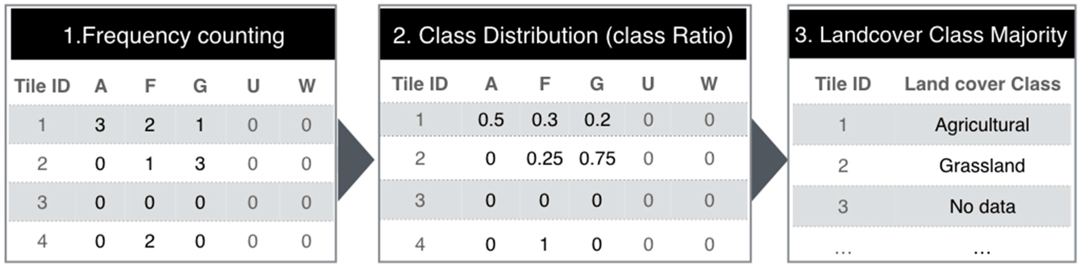
3.5. Application of Majority Class Filter Determination of Crowdsourced LULC Mapping

After the determination of free parameters, we use the majority distribution in a geospatial tile to ameliorate the effect of geographically non-informative (positional error) or misclassified images. Majority class filtering inspects the LULC types in neighborhoods to reduce uncertainty or unreliable information. To localize our analysis, we partitioned the study region into 30 m × 30 m (Landsat pixel size: Section 2.2) tiles and mapped each labeled Flickr image to a tile. To label the LULC class of each tile, the neighboring images were considered for majority class filtering by selecting the highest frequency LULC class in the given tile. Figure 6 shows an example of majority class filtering in the case study region of Sapporo City, Japan.

After obtaining the majority voting result, crowdsourced LULC mapping was used for training samples for LULC classification of the Landsat TM5 image using the maximum likelihood method (MLM), which is one of the most widely used methods for classification on account of its simplicity and robustness. The MLM classifier was trained using randomly sampled tiles for individual LULC types.

Training samples were collected on tile basis to reduce the redundancy and spatial autocorrelation. We uniformly selected the training samples from the tiles of each LULC type covering 70% of samples per class. The remaining 30% of tiles were used to validate the obtained LULC map. Here, we compare the classification result at each tile of the validation location [13].

Table 2. Confusion matrix for land use/land cover (LULC) classes from crowdsourced and Landsat TM5 imagery.

Observed Class from Crowdsourced Mapping	Predicted Class from Landsat TM5
	Class of Interest	Non-Class of Interest	Total
Class of interest	TP	FN	TP + FN
Non-class of interest	FP	TN	FN + TN
Total	TP + FP	FN + TN	N = TP + TN + FP + FN

shows the structure of a confusion matrix between the classification results from LULC classes from crowdsourced data and LULC classes of the Landsat TM5 image.

The observed classification accuracy of the crowdsourced map was determined by the diagonal elements of the confusion matrix. Chance agreement incorporated the off-diagonals of the confusion matrix (diagonals represented items correctly classified according to the reference data; off-diagonals represented misclassified items).

4. Results and Discussion

Through our experiment, we examined how effectively LULC types can be predicted using geotagged ground level images from Flickr. We used independent training and testing datasets as described in the previous section. The results showed that the naive Bayes classifier provides good performance for LULC classification.

4.1. Foreground/Background Segmentation Using Otsu Thresholding

The proposed image segmentation process is based on the Otsu threshold. We carefully selected the training image that has homogeneous features. For example, the image could have an obvious skyline or line structure to accurately segment the LULC features.

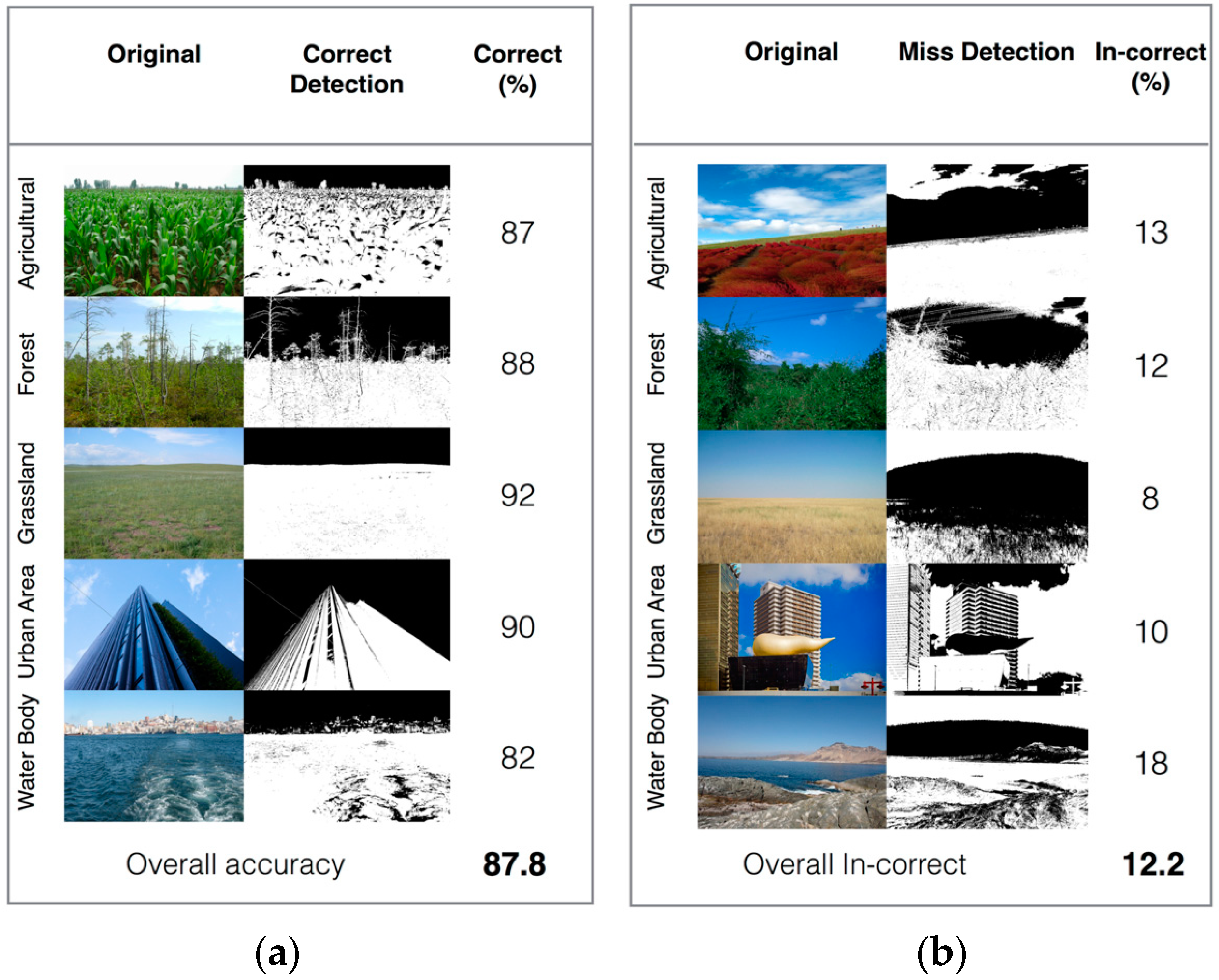
Sample results for different LULC types are shown in Figure 7. The obtained results clearly indicate that the white pixels identify agricultural, forest, grassland, urban structures, and water features in the original images. In Figure 7a, black pixels correctly identify background and other material present in the image (87.8% correctly detected). The misdetections sampled in Figure 7b show 12.2% of incorrect classifications. The background illumination, time of day, and angle of the captured image contributed to misdetection. In some images, detection of the skyline was difficult. The angle from which the image was obtained also had a significant effect on skyline detection [43].

4.2. Color, Shape, and Color Index Based Image Classification

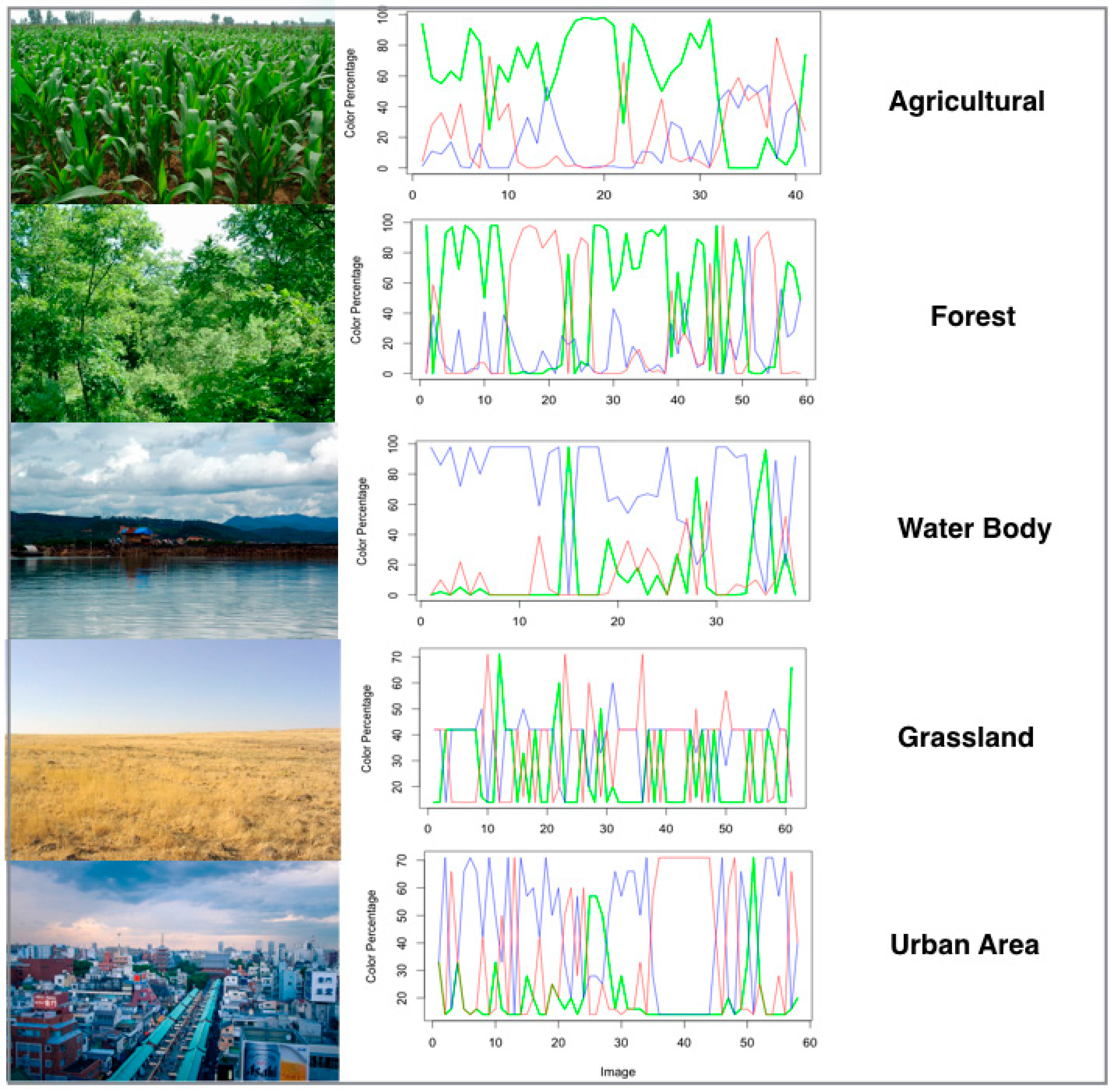
The segmentation method extracts relatively homogeneous regions. Based on the segmentation results, we removed the background from each image and calculated the feature images for further analysis. Manually selected training sample images were placed into the categories of agriculture, forest, water, grassland, and urban. Sample color feature histograms are shown in Figure 8. Classes with vegetation (agriculture, and forest) show a dominant green channel, while the water class shows a dominant blue channel. However, grassland and urban areas have no distinctive color channel patterns. This is possibly on account of the variation in color of the targeted feature.

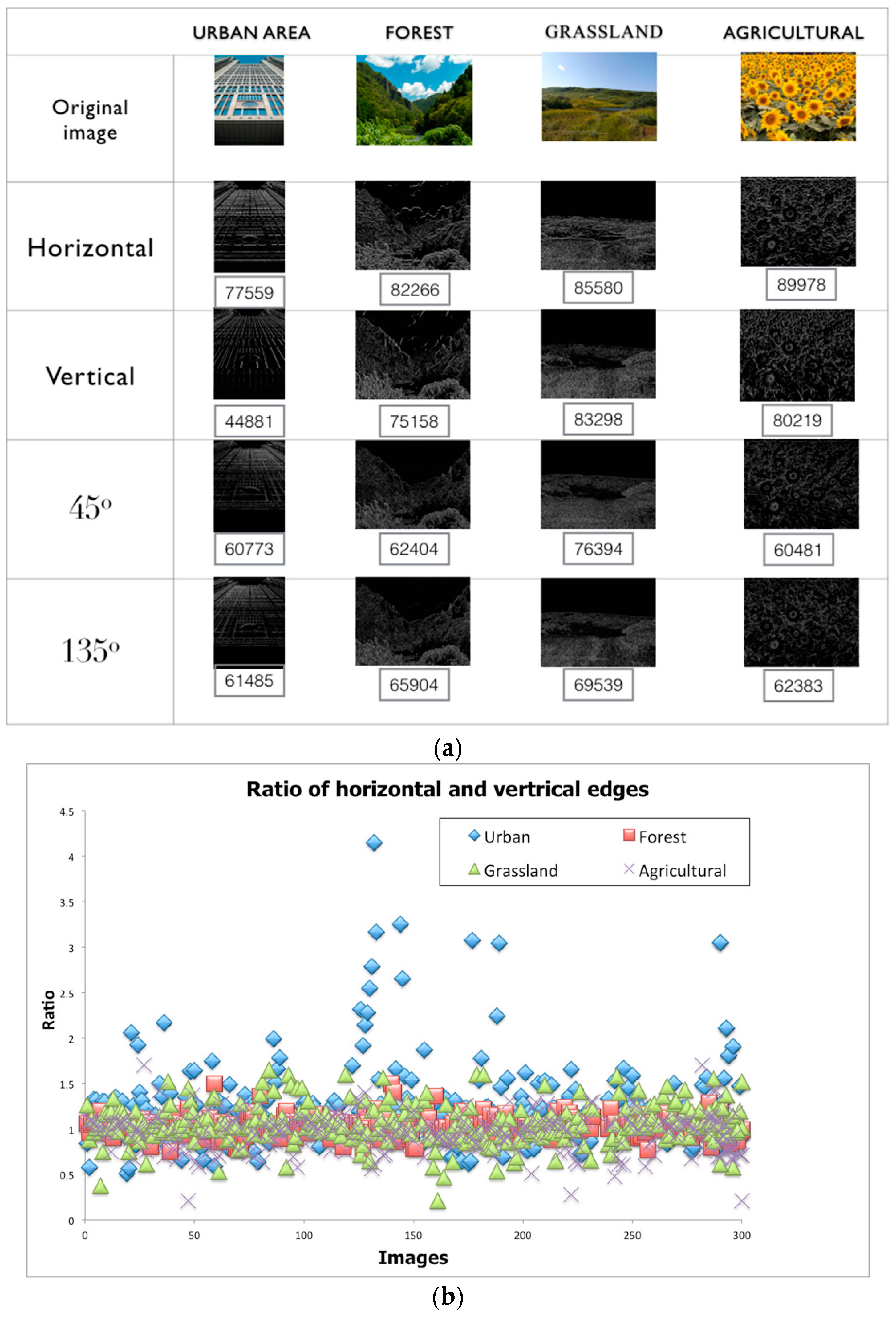
Sample results of thresholding the outputs of the linear oriented edge filters are shown in Figure 9a. We found that images of urban scenes have a much higher proportion of horizontal and vertical edges than other non-urban scenes (forest, grassland, and agriculture). Developed areas show a visible pattern (spikes in the ratio of horizontal and vertical edges in Figure 9b). One issue with edge histograms is that the edges of a building may have diagonal orientations on account of perspectival distortion.

We performed an initial comparison of VIs for plant and background features on the original color image, as shown in Figure 10. The greenness extraction approach combined the information provided by different vegetation indexes (VIs), as discussed in Section 3.1.2. We found that the ExG index successfully discriminated grassland, evergreen forest, and agriculture from the background; however, it separated deciduous forests with higher redness from other forests. ExR was useful for discriminating grassland from the background on account of its extraction of redness, soil, and residue. It was also effective at separating deciduous forests and evergreen forests. Nevertheless, it did not perform well for extracting dominant greenness (agriculture).

The NDI index could separate agriculture from soil and background. However, we found that illumination had a significant impact in not capturing the color of other vegetation categories (grassland, deciduous forest, and evergreen forest). The ExGR index appeared to accurately extract dominant greenness (agriculture) as long as the background and soil were detected as background in the segmentation. Figure 10 shows that ExG, NDI, and ExGR together separate the plant regions quite accurately from the soil and background. Both NDI and ExGR show the effect of separating forest and grassland. Hence, our combined VI feature extraction technique shows good results for separating different kinds of vegetation.

4.3. LULC Feature Classification Using Naive Bayes Classifier

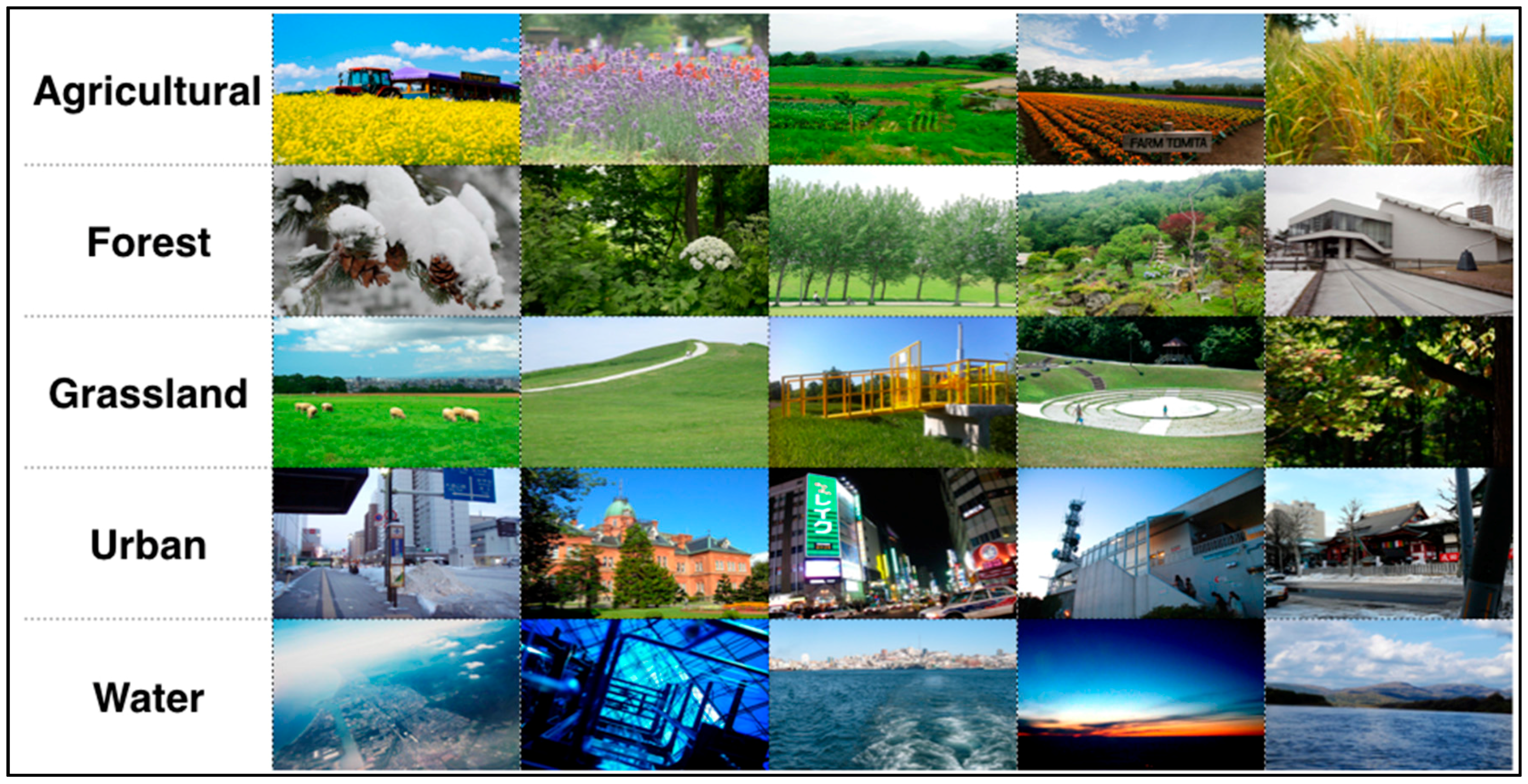
We tested the performance of the proposed approach in extracting five major LULC types (water body, urban area, grassland, forest, and agriculture) on labeled Flickr images. The naive Bayes classifier enabled subjective definitions to be described in terms of our color, shape, and color index features. We arbitrarily selected training LULC images. We calculated a set of parameters from each training set and then applied those parameters to classify the images in the test set. Figure 11 shows sample images labeled by the naive Bayes classifier.

4.4. Measuring Performance of the Naive Bayes Classifier

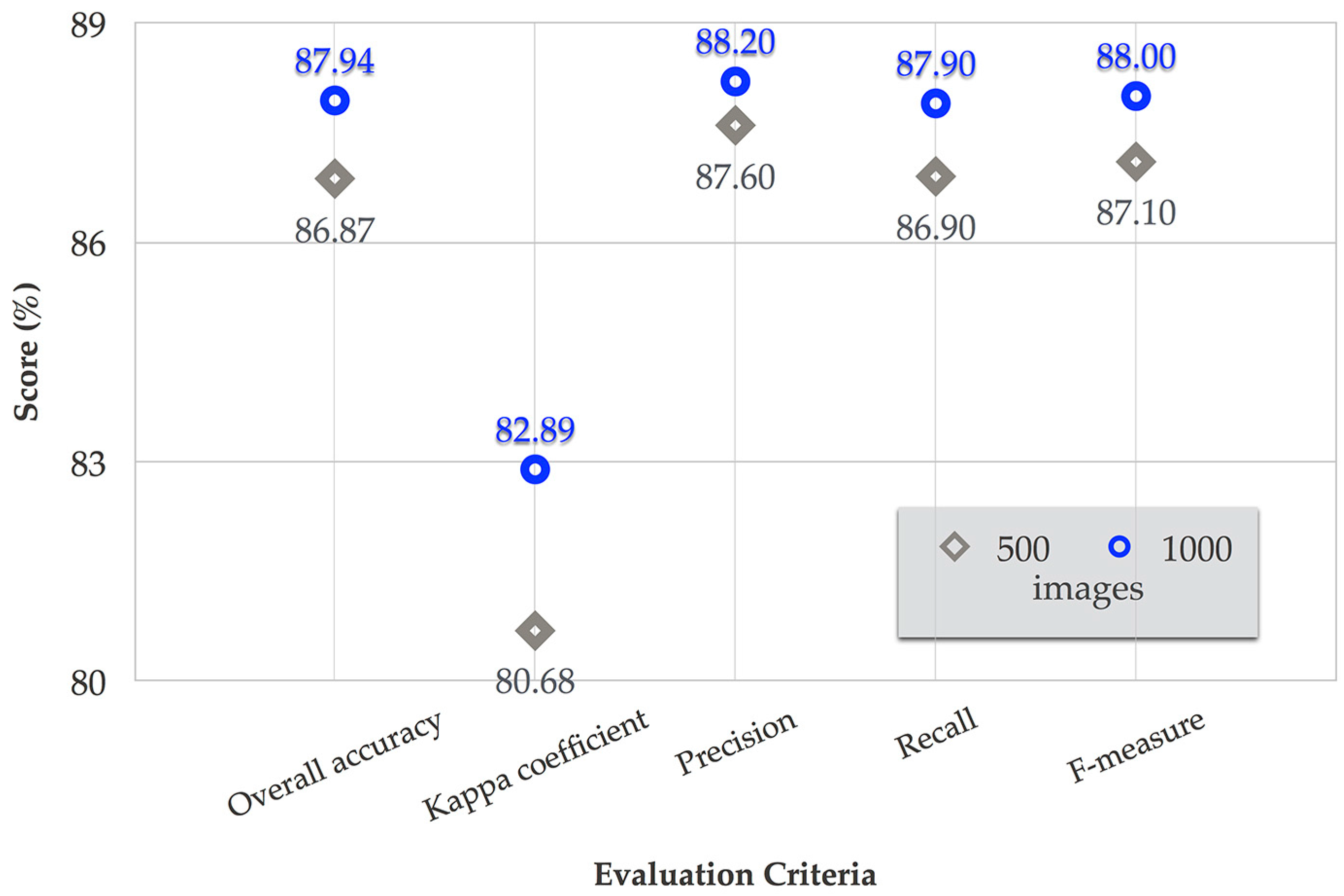
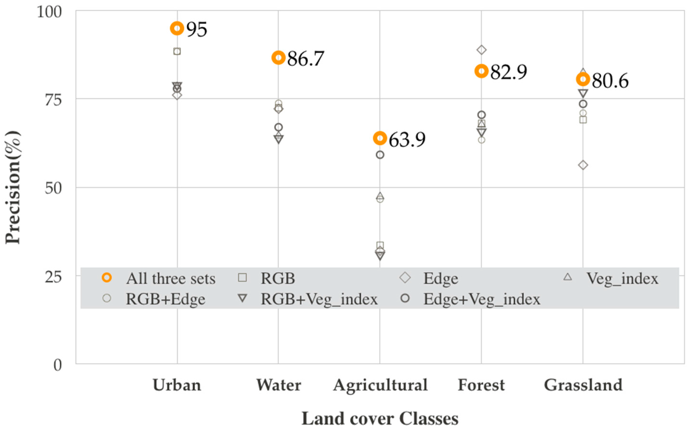
We performed a model evaluation using precision, recall, f-measure, ROC curve, kappa coefficient, and overall accuracy (Figure 12 and Figure 13 present the results). The availability of classification accuracy depended on the training dataset size: an increase in the training dataset size increased the accuracy. Thus, more training data may further improve LULC classification. Figure 12 shows that at least 1000 training image samples are required for naive Bayes to provide a satisfactory LULC class estimation. The performance obtained using 1000 training samples are clearly better than the results with 500 training samples. With 1000 training samples, we obtained an overall accuracy, kappa coefficient, precision, recall, and f-measure of 87.94%, 82.89%, 88.20%, 87.90%, and 88%, respectively.

Figure 13 shows the system performance with different combinations of color, edge, and VI features. The combination of multiple features contributed to the discrimination between different LULC types. The urban area, water, forest, and grassland categories are classified with satisfactory accuracy (>80%). However, agricultural shows only 63.9% positive classification, primarily because of the misclassification of agricultural areas as other classes (36.1%). This misclassification may result from the relatively small number of training samples in the dataset and heterogeneity features in the agriculture images.

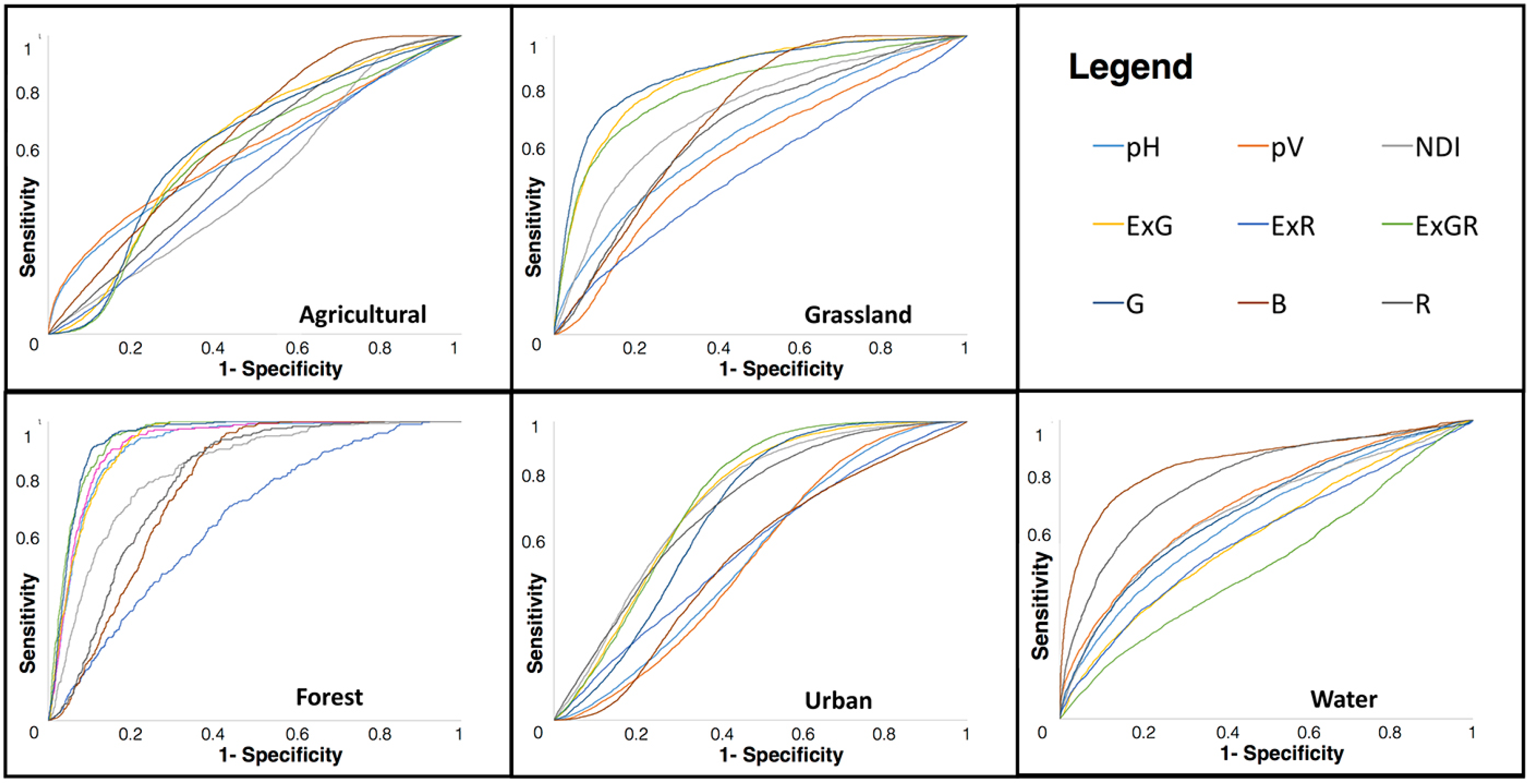
ROC analysis was performed to estimate the classification accuracy (sensitivity against single-specificity on a per-category and per-feature basis). Accordingly, we selected a threshold for a feature above which a labeled LULC class was considered positive. The area under the ROC curve (AUC) evaluated the classifier over all cutoff points, giving better insight into how well the classifier can distinguish the classes. An area under the ROC curve of 0.5 indicated a random prediction.

For each LULC class, we compared correctly classified relevant images against incorrectly classified images. In the case of water, the ROC curve and area under the ROC curve for the blue descriptor performed well. The green descriptor showed outstanding performance (ExGR: 0.944 and G: 0.943) in discriminating grassland and forest from other classes, as shown in Figure 14. Urban images can be effectively differentiated by the vertical edge orientation descriptor. However, ROC curves for agricultural images are poorer for every descriptor on account of the heterogeneity of the objects (e.g., flowers, cropland, and paddy fields), which affected the classifier performance.

In summary, we investigated the application of crowdsourced data to LULC classification. We employed the renowned naive Bayes classifier model on account of its speed, efficiency, capability of handling large amounts of data, and insensitivity to irrelevant features. We determined that our combined feature descriptor yielded good overall accuracy of 87.94% of the test dataset of LULC classification. The use of features sensitive to vegetation characteristics is particularly useful in reducing the uncertainty of classification of the crowdsourced images.

4.5. Crowdsourced and Landsat TM 5 Based LULC Classification

After classifying individual images, we performed majority class filtering to obtain LULC predictions for neighborhoods to reduce uncertainty and ignore unreliable information. Images distributed in 30 m × 30 m areas were considered for majority class filtering by selecting the highest frequency. From this result, we obtained LULC classes for each tile in the map.

Table 3. Number of tiles in each of the classes from crowdsourced LULC mapping.

Crowdsourced LULC Class	Number of Tiles
Agricultural	744
Forest	120
Grassland	345
Urban areas	4050
Water bodies	93
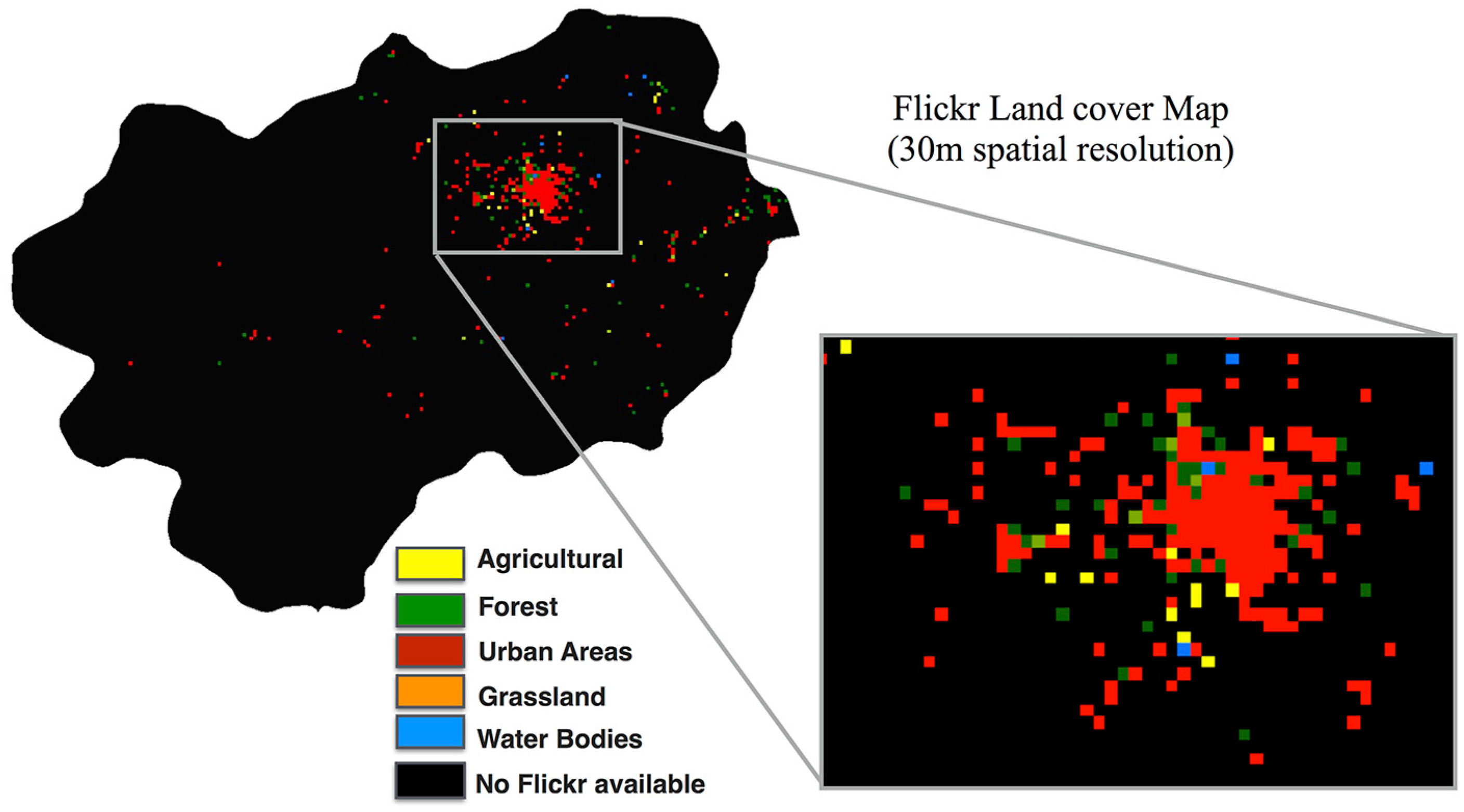
Total	5352

shows the obtained number of tiles in each of the LULC classes. Urban areas have the highest number of tiles for the overall area, followed by agriculture, grassland, water bodies, and forest, respectively.

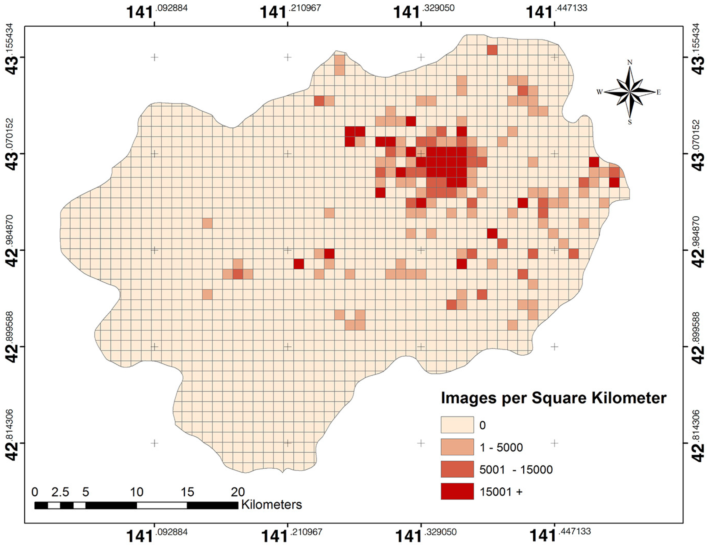
Figure 15 shows the LULC map obtained from Flickr imagery. It contains the majority LULC class for the area in Sapporo City, Japan. The Flickr LULC map occupies approximately 10% of the total area, whereas other areas have no Flickr images. However, the urban areas have the highest distribution of the crowdsourced LULC map. This agreement could be due to the density and distribution of available images being sufficiently high in a particular tile [16].

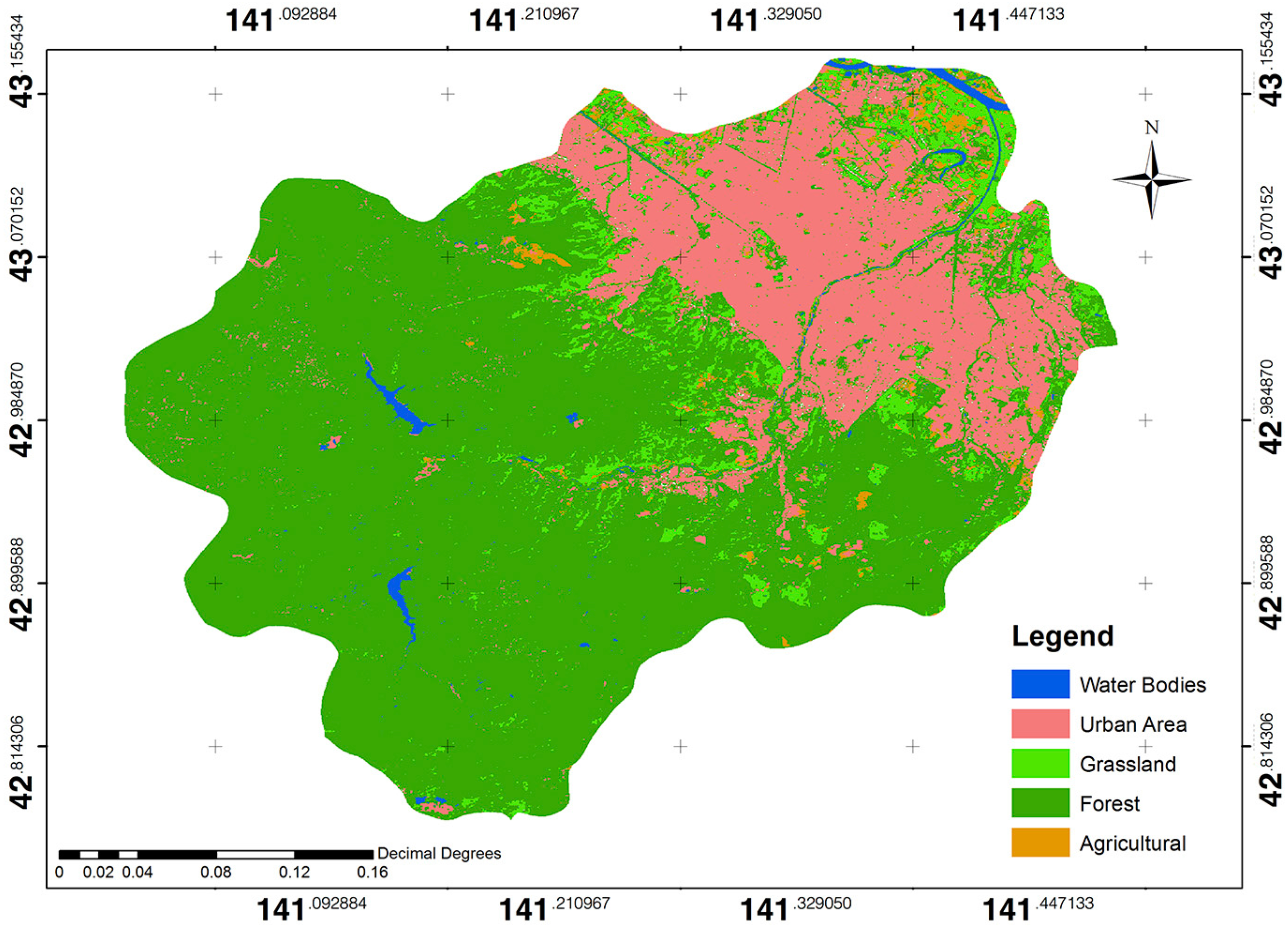
After filtering the individual tile, we performed supervised classification on the Landsat TM5 image using the majority filtered crowdsourced LULC tiles as training and validation datasets to acquire the LULC map. Figure 16 shows the Landsat TM5 based LULC mapping, which was trained by Flickr images. The accuracy evaluation was performed to compare the accuracy between the crowdsourced and Landsat TM5 LULC mapping coverage of the Sapporo City area.

Table 4. Classification accuracy of Landsat TM LULC mapping.

Land Use/Land Cover Class	User’s Accuracy (%)	Producer’s Accuracy (%)	Overall Accuracy (%)	Kappa Coefficient
Agricultural	64	83	70%	0.625
Forest	68	53
Grassland	61	64
Urban areas	85	69
Water bodies	72	94

shows the accuracy assessment, which was calculated using the confusion matrix obtained to assess the quality of the classification [18]. The obtained overall accuracy and the kappa coefficient are 70% and 0.625, respectively, which are mostly driven by urban areas. This implies that crowdsourced images can support ground truth information as training/validation data for urban/non-urban mapping.

In short, the proposed approach uses the crowdsourced (Flickr images) dataset and produces training and validation data for use in various LULC applications. However, the performance of the image processing chain may be limited, particularly over a large area and by variety of classes requiring a sufficient quality of reference data.

5. Conclusions

In this paper, we proposed the use of Flickr images for LULC classification to automatically recognize specific types of LULC from visual properties of crowdsourced data. This method (the combination of thresholding, color, shape, and color indices) yielded good classification accuracy. The combined feature descriptor method with 1000 training images provided 88% accuracy over five LULC categories. Integration of color index descriptors with the naive Bayes classifier improved the separation of different types of vegetation. Especially for areas with green vegetation, the proposed strategy outperformed the simpler color and shape index combination in terms of accuracy. The number of training samples greatly affected the classifier performance. Increasing the number of training samples led to increased classification performance. Further improvement may be possible using larger training sets. However, the results show that an acceptable accuracy level can be obtained using a minimum number of training samples.

As a whole, these findings provide insight into the applicability of probabilistic classifiers and the number of training samples required when implementing an object-based approach to LULC classification using a large crowdsourced dataset. The results also highlight the utility of integrating color indices with machine learning. The crowdsourced data can be potential training samples for various LULC applications. We assessed the classification performance for both image-based recognition and mapping-based classification. Because we tested all possibilities to obtain the highest accuracy from image recognition, we could then map these reference images in terms of spatial distributions using majority voting approach.

For image recognition, we performed a model evaluation using precision, recall, f-measure, ROC curve, kappa coefficient, overall accuracy, and ROC. For mapping classification, we validated the classification result using 30% of tiles of each LULC class with equal spatial distributions in a particular area. The accuracy evaluation was performed to compare the accuracy between crowdsourced and Landsat TM5 LULC mapping covers of the Sapporo City area. The accuracy assessment was calculated using the confusion matrix obtained to assess the quality of the classification of LULC mapping.

This approach is extensible and can be useful for specific areas that especially depend on the availability of images. Its ultimate benefit may be the possibility of automatically monitoring heterogeneous/subclass classification or noise image removal, such as agriculture (flower, cropland and rice paddies), forest (deciduous and evergreen forest), long-term vegetation changes (changes in agricultural, forest, and grassland), and other objects (face/people and animals). Social media can support data sources for both urban and natural resource planning, allowing modeling and identification of historic and new identifications of LULC in a relatively inexpensive and near-real-time manner.

Another application of the proposed approach is validating or updating of existing LULC maps using social sensing, which requires rigorous sampling design. The images could complement an already existing validation dataset, which would be less costly and time consuming than the traditional field survey methods. In sum, this work marks an initial step toward improving our ability to classify, detect changes in, and validate LULC maps obtained by remote sensing through the use of social-sensing databases. Moreover, it may provide information that can be helpful if combined with other crowdsourced data, such as Panoramio, Facebook, and Twitter [11].

In future work, to improve efficiency and obtain additional image feature descriptors, we plan to use more sophisticated texture extraction techniques [19,31] with other machine learning models, such as neural networks, random forest, and support vector machines, as well as other sources of geotagging crowdsourced data [11]. Finally, we intend to extend the scope of our approach to investigate how well naive Bayes and other classifiers can be trained using Flickr or other social media images from one region to classify LULC in other regions.

This study considered only the location of the image acquisition. However, most cases can be performed by majority voting to represent LULC classes. We plan to advance our work by considering the direction of the image to increase the classification efficiency. We hope that the idea of observing natural and man-made features through social-sensing photo-sharing websites can foster a greater understanding of the earth-surface properties and characteristics in spatial and temporal terms.