
Effects of the Post-Olympics Driving Restrictions on Air Quality in Beijing

1
State key laboratory of petroleum resources and prospecting, China University of Petroleum, Beijing 102249, China
2
Department of Geochemistry and Environmental Sciences, China University of Petroleum, Beijing 102249, China
3
State Key Laboratory of Urban and Regional Ecology, Research Center for Eco-Environmental Sciences, Chinese Academy of Sciences, Beijing 100085, China
*
Author to whom correspondence should be addressed.
Sustainability 2016, 8(9), 902; https://doi.org/10.3390/su8090902
Submission received: 21 July 2016
/
Revised: 29 August 2016
/
Accepted: 1 September 2016
/
Published: 6 September 2016
(This article belongs to the Special Issue Air Pollution Monitoring and Sustainable Development)
Abstract
:To reduce congestion and air pollution, 20% driving restriction, a license plate-based traffic control measure, has been implemented in Beijing since October 2008. While the long-term impacts of this policy remain controversial, it is important to understand how and why the policy effects of driving restrictions change over time. In this paper, the short- and long-run effects of the 20% driving restrictions in Beijing and the key factors shaping the effects are analyzed using daily PM10 pollution data. The results showed that in the short run, 20% driving restriction could effectively reduce ambient PM10 levels. However, this positive effect rapidly faded away within a year due to long-term behavioral responses of residents. A modified 20% restriction, designed to replace the original 20% restriction system since April 2009, which is less stringent and provides more possibility for intertemporal driving substitution, has shown some positive influence on air quality over the long run comparing with that under the original policy design. Temporarily, the more stringent the driving restriction was, the better effects it would have on air quality. In the long-run, however, the policy was likely to cause a vicious circle, and more stringent policy might induce stronger negative incentives which would result in even worse policy effects. Lessons learned from study of the effects of driving restrictions in Beijing will help other major cities in China and abroad to use driving restrictions more prudently and effectively in the future. Decision-makers should carefully consider the pros and cons of a transport policy and conduct the ex-ante and ex-post evaluations on it.
1. Introduction
Air pollution and traffic congestion remain serious problems in major cities worldwide. In response to this, substantial policy measures, such as driving restrictions, bus priority, carpooling, gasoline taxes, parking fees, and road pricing, have been designed and implemented in those cities. Among its policy alternatives, a driving restriction, as a command-and-control measure, is relatively easy and inexpensive to implement, enforce and understand [1,2], and therefore is particularly favored by policy makers in developing cities, most of which are Latin American cities. In November 1989, for example, authorities in Mexico City imposed a regulation, Hoy-No-Circula (HNC), banning each car from driving one weekday per week based on its last digit of license plate. Similar driving bans were introduced in São Paulo, Bogota, and Santiago thereafter. In spite of its popular adoption, the regulation remains controversial. Some argue that instead of achieving the policy goals for reduction of congestion and air pollution, the regulation is in fact inefficient and unfair [3]. Evidence shows that the HNC in Mexico City has not improved air quality due to the fact that the mode shift has not been environmentally friendly, more cars in circulation and higher pollution levels [2,3]. Further, Gallego et al. (2013) look at the impact of HNC on air quality in Mexico City and report the positive short-run effect and rapid adaptation process [4]. Although New York City once proposed license plate rationing as an alternative to congestion pricing, such measures have not been implemented in any city in the United States. In EU countries, instead of driving restrictions, road pricing and low emission zone (LEZ), a policy restriction on vehicle emissions in certain areas, are more popular and have been implemented in many cities [5]. Although practical implementations of driving restrictions do exist in EU cities, most of them are temporarily employed during mega events and peak pollution episodes, such as driving bans issued in London during the 2012 Summer Olympics, and odd-even scheme imposed in Paris during the air pollution episodes in March 2014 and March 2015. One exception is Athens, which has imposed permanent odd-even driving restrictions in the center of the city (“ring”) since June 1982, which has been criticized in the sense that while it reduces traffic and pollution in the ring, it results in considerable traffic and pollution problems at the perimeter of the ring [6].
The recent decade has witnessed a dramatic increase in the number of vehicles in China, especially in Beijing, where the fleet of motor vehicles has increased over ten times. With vehicles being the major local emission contributor [7], and with the remarkable amount of regional transport of industrial pollution, Beijing is now suffering from the increasing numbers of haze events, which rapidly raise high levels of public health concerns. To tackle the severe automotive pollution problems, driving restriction policies have been introduced in Beijing. Driving restriction was first introduced in the form of odd-even scheme in Beijing during the 2008 Olympics. Since the odd-even program achieved significant improvements in congestion and air quality during the 2008 Olympics, a less stringent post-Olympics version, the 20% driving restriction (also termed as “one-day-per-week” scheme in some literature, e.g., [8]) was adopted in Beijing since 11 October 2008, and evidence of high compliance has been observed [8]. But being a temporary implemented measure, could the success of the odd-even scheme during the Olympics assure the positive policy effect of the 20% restriction version in the long run?
While there are great concerns at home and abroad about the environmental effects of the odd-even driving restriction during the Beijing Olympics, and most of which support the significant positive effect of the policy [9,10,11,12,13], much less attention has been paid to the post-Olympics 20% restriction scheme. Among them, some point out that given the rapid improving affordability of automobiles to Chinese households, such driving bans can hardly suppress vehicle use and slow down vehicle fleet growth even in the short run [14], some address the short-run effect and find no evidence that the restrictions have improved air quality [10,15], while others report the improvement of air quality in the short run [8,16].
Two key factors highlighted by the literature that may affect the effectiveness of a driving restriction are intertemporal driving substitution in the short run and adjustment of car ownership in the long run [17]. Intertemporal driving substitution, driving vehicles during hours of the day and days of the week when restrictions are not in place [18], could be a fast and effective short-run adaptation of residents to a policy shock. Davis (2008) finds evidence that weekend and late night air pollution increased relative to weekdays, which suggests intertemporal substitution toward hours when HNC is not in place [2]. Lin et al. (2014) note that the stringent design in Beijing and less restrictive version in Tianjin during the 2008 Olympics might have led to different degrees of driving substitution, thus causing the different air quality effects of the odd-even driving restrictions, i.e., significant decrease in PM10 levels in Beijing and no effect in Tianjin [17]. Buying a second car, however, is usually a kind of long-run adaptation, especially for families that originally do not plan to buy an additional car, and thus need time to rearrange their household budget. A long-term effect could be observed while most of the affected adjusted to the policy [4].
Since haze pollution continues to be an acute problem in Beijing, especially after the extremely severe and persistent haze events in the first quarter of 2013 [19], the Beijing municipal government is discussing whether instead of the 20% restriction the odd-even rule should be made permanent, and many other cities in China and abroad suffering similar congestion and pollution problems are also considering the possibility of long-term use of driving restrictions. Therefore, it is important to understand how the effects of driving restrictions change over time. So far, though, little empirical evidence has been provided to understand the short- and long-term air quality impacts and to address the underlying behavioral influencing factors in domestic driving restriction studies. To our knowledge, the study by Chen et al. (2013) is so far the only one looking at the environmental impacts of driving restrictions in China from both short- and long-term perspectives [9]. However, with the odd-even scheme being one of their major interesting, their study mainly focuses on the impacts of a number of temporary measures taken by China to improve air quality before and during the 2008 Beijing Olympics. The post-Olympics driving restriction has been treated as a subsidiary measure, the impact of which has been integrated to the impacts of the Olympic efforts. Therefore, the long-run effect of the 20% restriction program remains vague.
The contribution of this paper is to address the short- and long-run air quality effects of the 20% driving restriction in Beijing and to identify the key factors shaping the effects, following the methods of Gallego et al. (2013) [4] while using PM10 as the indicator pollutant. We find that in the short run, 20% driving restriction can effectively reduce ambient PM10 levels, but this positive effect rapidly fades away within a year due to long-term behavioral responses of residents. This paper is organized as follows. Section 2 briefly introduces the 20% driving restrictions in Beijing and puts forward hypotheses on the policy impacts. Section 3 describes data collection and methodology. Section 4 reports results. Conclusions, discussion, and policy implications are presented in Section 5.
2. The 20% Driving Restriction Schemes and Empirical Hypotheses
2.1. The 20% Driving Restrictions in Beijing
Beijing is the first city in China to implement driving restriction policy. In order to reduce congestion and air pollution during the 2008 Olympics, along with a number of radical and temporary measures, such as plant closure, a stringent driving restriction based on odd-even license plate was implemented in Beijing during the mega sports event. Evidence of reduction of congestion and mobile source pollution was confirmed during this period [9,10,11,12,13]. The benefits of such restriction seemed so attractive that Beijing soon decided to resume with a similar, but less restrictive, 20% driving restriction as the major post-Olympics environmental and transportation management measure [14], which bans every vehicle, except police cars, ambulances, fire trucks, buses, taxis, school buses and vehicles with special permits, from driving one weekday per week based on the last digit of its license plate.
The restriction was adopted on October 11, 2008. Under this regulation, roughly 20% of cars are taken off roads on each weekday. It was applicable within the 5th Ring Road, from 6 a.m. to 9 p.m. for private cars and round the clock for government and business vehicles. On 10 April 2009 small changes were made to the restriction, with the effective hours changed to 7 a.m. to 8 p.m. on weekdays for private cars [10]. The adjusted driving restriction could provide more convenience thus more possibility for intertemporal driving substitution compared with the original design.
2.2. Empirical Hypotheses
Based on the empirical results of driving restrictions in Latin cities, two behavior-based hypotheses on the policy results in Beijing are developed and to be tested in this study. First, though driving substitution could be adopted as a quick response, the overall opportunities of adaptation of vehicle users are limited in the short run [18]; in this case, Beijing might have experienced some reduction in ambient PM10 level at the beginning of the policy implementation. Second, in the long-run, the policy effect could go either direction. On one hand, there could be long-term positive policy effects on air quality, if on the restricted weekdays most of the affected drivers shifted to the environmentally-friendly modes such as public transits and carpools, and if households who intended to buy a car postponed their car buying plan because of the restricted use. It is also possible that some drivers might cut out their trips on the restricted weekdays, which might increase the risk of social exclusion. On the other hand, earlier policy effect would gradually fade away if households tend to respond to the policy by buying a second car rather than shifting to environmentally friendly modes.
3. Data and Methods
3.1. Data Collection
Data used in this study include ambient particulate matter (PM10) concentration, meteorological data such as temperature, humidity, precipitation, wind speed, wind direction, and other variables to control time changing factors such as time trend variable, months of a year and days of a week.
3.1.1. Time Window
In order to disentangle the effect of the 20% driving restriction from the effect of other time-varying factors that influence air quality in Beijing, a relatively narrow time window, October 2006–October 2010, which is four years around the implementation of the policy is used. And other reasons of using this time period are presented as follows. Beginning in 2011, a “vehicle quota” policy was adopted by Beijing municipal government, which put a monthly cap of around 20,000 on the numbers of vehicle license plate issued officially; this must have confounding impacts on air quality while the effect of driving restriction is addressed. And also, by using this time period, we avoid data bias caused by a shift of monitoring stations happened in Beijing in early 2006, which had been providing data for averaging the reported city-level air quality.
3.1.2. API Values and PM10 Concentrations
Daily Air Pollution Index (API), which is calculated based on the concentration of the primary pollutant of the day, is the only accessible public data in Beijing during the research time interval. Chinese API has been used in several scientific studies [8,9,10,17]. While the credibility of Chinese API has been questioned [20], study of Chen et al. (2013) find no obvious evidence of gaming of the API in Beijing according to a stable correlation between API, AOD (aerosol optical depth), and visibility [9].
During the research time interval, the overwhelming majority of the daily primary pollutant is PM10. Therefore, PM10 concentration is used in this study to identify the environmental impact of the policy. Vehicle emission is one of the major pollution sources of particulate matter in Beijing. Studies indicate that, with time going by, vehicle emissions contribute 5%–20% and 6%–28% of the PM10 and PM2.5 concentrations in Beijing, respectively [7,21,22,23]. According to the most recently report of Beijing Municipal Environmental Protection Bureau (BJMEPB), vehicle is the highest local emission contributor to PM2.5 with the contribution rate of 31.1%. Although it might not as an ideal proxy for car use as pollutants such as CO [4], PM10 could still be used as an important ambient indicator of vehicle emissions in Beijing.
Daily city-level API of Beijing during the year of 2006–2007 was downloaded from the online data center of Ministry of Environmental Protection of China (MEP, www.zhb.gov.cn). Daily station-level API during the year of 2008–2010 is accessible from the website of BJMEPB (www.bjepb.gov.cn). After the first shift of monitoring stations in Beijing in 2006, another station change happened in the beginning of 2008, while three new stations were added in the list. In order to enhance the data comparability, daily station-level API data during 2008–2010 are collected and averaged from the original eight stations that were used to estimate daily average air quality in Beijing during 2006–2007.
Daily concentrations of the primary pollutant are retrieved from API. During the research time interval, there are three kinds of API data that need to be identified and treated differently. Firstly, on 87.9% of the days during the four-year time window when the primary pollutant is PM10, the mass concentrations of PM10 could be retrieved directly from the reported API. Secondly, on 2.2% of the days when the primary pollutant is SO2, PM10 concentration is retrieved from the reported API of SO2, which is used as the upper-bound concentration of PM10. Thirdly, on 9.9% of the days when the air quality is really good and API is less than 50 and no primary pollutant is reported, the reported API would be used as the upper-bound index for retrieving PM10 concentration. This treatment might slightly underestimate the effect of policy on PM10 reduction, or in some cases slightly overestimate the policy effect on PM10 increase. Table 1 introduces the breakpoints of API and the corresponding air pollutant concentrations. And the conversion between API values and air pollutant concentrations is calculated using the following formula [24].
where —air pollution index of pollutant x, —the concentration of pollutant x, —API value of the breakpoint j, —API value of the breakpoint j+1, —the concentration of the breakpoint j (corresponding to ), —the concentration of the breakpoint j + 1 (corresponding to ).
We focus on the data of the whole weeks instead of the data of the weekdays, despite of the fact that the driving restriction is only implemented during weekdays. The reason is that in China the API is reported once a day with a period from 12 p.m. of the previous day to 12 p.m. of the current day, which is different from the concept of a natural day. e.g., the API estimation of Monday includes the pollution information of Sunday, while the driving restriction is not at place. And likewise, pollution of Friday evening peak, which is the most congested and polluting peak among a week, is included in Saturday data. Therefore, in this study we focus on the whole group data which could provide more comprehensive pollution impact information.
3.1.3. Meteorological Data
Beijing sits ringed by mountains on its north and west, and is surrounded by industrial cities of Hebei Province in the south and east. With this unique geography, air pollutants are easy to be trapped and difficult to be dispersed, and regional pollution transported by the southerly flow can even worsen the pollution situation in Beijing. Therefore, meteorological variables are critical to be controlled in this context. Temperature, humidity, precipitation, wind speed and wind direction are collected from Weather Underground (www.wunderground.com), a website reporting real-time city-level meteorological data around the world, data of which have been used in several scientific studies [10,12,17].
3.2. Evaluation Method
Davis (2008) addresses the effect of HNC on air quality in Mexico City [2], which is the first empirical study of effect of driving restriction using ambient pollutant data. To look at the temporal heterogeneity of the effect of HNC, Gallego et al. (2013) developed a strategy to reveal the dynamics during the months after the policy implementation [4].
To understand the short- and long-run responses of households to the 20% restriction scheme in Beijing and the consequent air quality impacts, this study follows the method of Gallego et al. (2013) [4] and tests the robustness of the estimates. Time trend and seasonal effects are controlled to avoid spurious regression.
We use the following model to estimate the influencing powers of explanatory variables, especially the policy indicators, on daily PM10 concentrations in Beijing during October 2006–October 2010.
Yt is the daily city-level ambient PM10 concentration in logs, the outcome of the policy. is an indicator variable equal to 1 after the implementation of the 20% driving restriction since 11 October 2008; is a dummy that takes the value of 1 after the policy adjustment since 11 April 2009. Xt is a vector of covariates including month of the year (to control seasonal pattern of air quality), weekday dummy (Tuesdays through Fridays = 1, Mondays are excluded from the weekday group since their data include the pollution information of Sundays, as mentioned in Section 3.1.2), weather variables (including temperature, humidity, precipitation, wind speed, and wind direction), dummy variable of odd-even driving restriction that carried out during 17 August–20 August 2007 (a four-day test, exactly one year prior to the 2008 Games, for traffic reduction and environmental improvement) and 20 July–20 September 2008 as one of the major temporary air-quality improving measures during the 2008 Beijing Olympics (Studies report that the air quality improvement in Beijing was not obvious until the start of the Olympics [9], therefore the effects of other radical measures such as plant closure could be narrowed to the time period of the Games, i.e., the effects of which could also be captured by this dummy variable). “t” is a linear trend that controls for unobserved determinants of air quality that vary across time. “dt” are the monthly dummies for several months after policy implementation to capture the adaptation phase following policy implementation. is the error term. and would be the average long-run impacts of the 20% driving restriction and the policy adjustment on ambient PM10 level, respectively.
Other variables that might have influence on the level of economic and transportation activity, such as GDP and gasoline prices, were also tested but found not to be significant and, therefore, are not included in the specification.
4. Results and Analysis
4.1. Air Pollution during the Studied Time Window
Table 2 and Figure 1 indicate the API levels and the corresponding health effects, as well as the daily PM10 levels in Beijing during the studied time window, respectively.
Table 2 shows that people suffered health damage caused by air pollution (API > 100) in more than one quarter of the days during these years. The year 2008 seems to have the similar pollution pattern to the other years, except for more level I days, indicating more clean days among the summer Olympics.
As we can see from Figure 1, there is a plunge of PM10 level during June–September 2008, indicating the impacts of the radical measures, mainly the odd-even driving restriction and plant closure, adopted to improve air quality during the Olympics in 2008. The following period of time seems to have a slight decrease in pollution level as compared to the former years, with at least lower level of monthly maximums, which might be attributed to the implementation of the 20% driving restrictions. As time goes by, though, the pollution levels soon return to the levels before the year 2008, possibly indicating the fade-away of the instant effects of the 20% driving restriction policy.
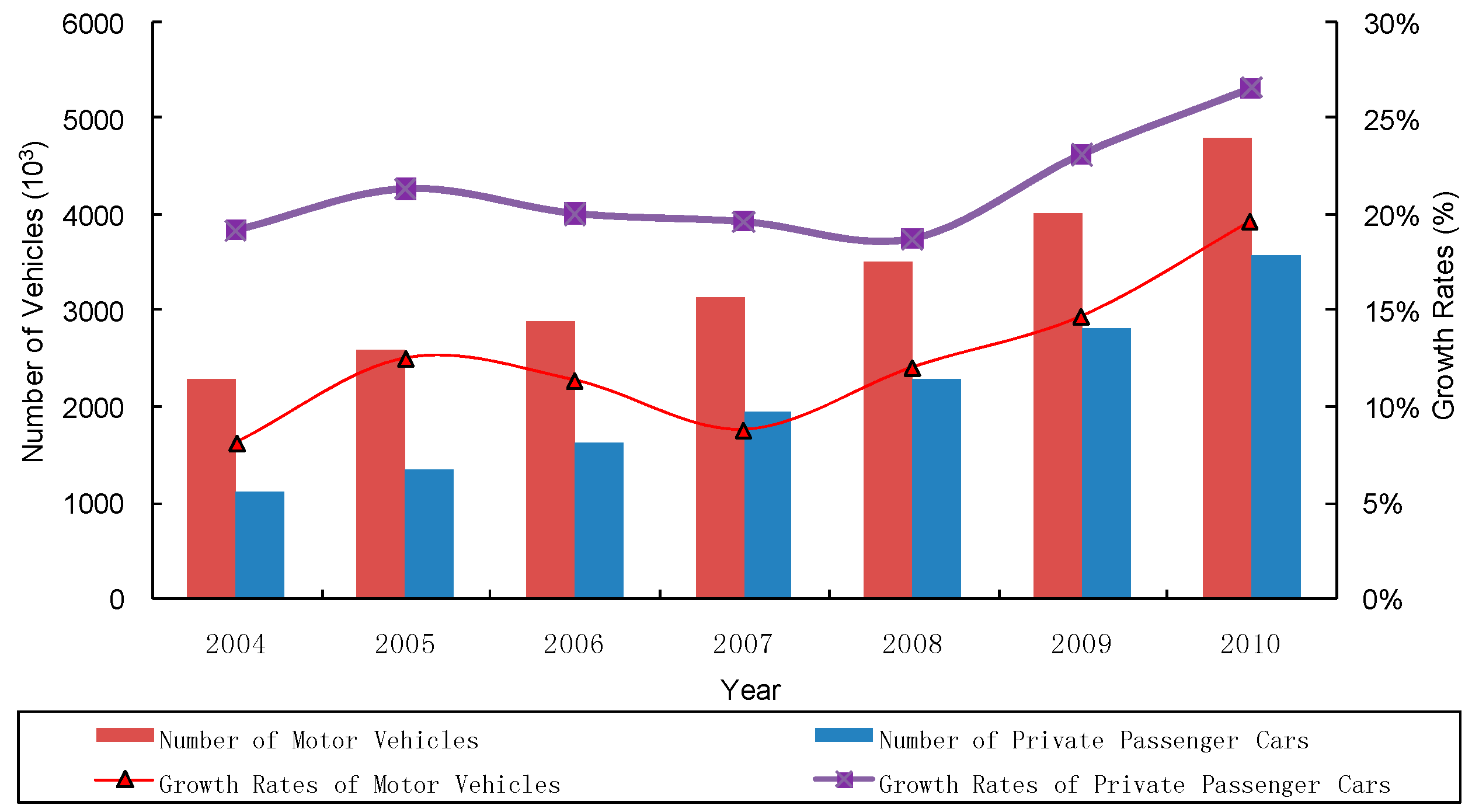
4.2. Rapid Growth of the Motor Vehicle Fleet in Beijing
The fleet of motor vehicle in Beijing rapidly increased from 2.30 million in 2004 to 4.81 million in 2010 (Figure 2). The results showed that the average increasing rates of motor vehicles and private passenger cars were roughly around 10% and 20% during 2004–2008, respectively, while in 2009 and 2010, the growth rates of motor vehicles jumped to 14.7% and 19.7%, respectively, and the growth rates of private passenger cars jumped to 23.1% and 26.5%, respectively. The rapid increasing of motor vehicle fleet is very likely to be triggered by the 20% driving restrictions implemented since October 2008. This observation supports our second hypothesis that in the long run, households tend to respond to the policy by buying an additional car.
4.3. Temporal Impacts of the 20% Driving Restrictions
Table 3 estimates the monthly effects of the 20% restrictions on air quality, with the dependent variable as the logs of daily city-level PM10 concentrations during the 4-year time window.
Fourteen regressions are reported in Table 3, numbered from (0) to (13). In the model (0) that does not include the monthly dummies, the average long-run impact of the 20% restriction policy is not significant. This seems to indicate that the policy has no effect on air quality. However, the statistical significance of the long-run impact changes when gradually adding monthly dummies into the model, where the short-term policy impacts are captured therefore weigh less in the average long-term impact. In the specifications containing more than two monthly dummies, all the coefficients of the 20% restriction are positive, and further, all the coefficients of the 20% restriction are significant while more than seven monthly dummies are included in the specifications. These indicate that the policy in the long-run might have increased the ambient PM10 level. It supports one of the two directions of our second hypothesis that the adaptation behavior is highly associated with the purchase of additional vehicles rather than the environmentally-friendly responses such as shifting to public transits, or cutting out trips. This adaptation behavior hypothesis is also supported by the rapid increasing trend of motor vehicle fleet after policy implementation. As more month indicators are included in the models, the monthly dummies become significant, and the explanatory powers of the models become stronger. Although the coefficients of determination are relatively small, we can see clear trends of the short-term effect: the coefficients of the first 10 months are negative and significant, and then the effects fade away as the following months are not significant, and the signs of the 12th and 13th months are turning to positive. This indicates that the 20% restriction in the short run has reduced the ambient pollution level, which supports our first hypothesis. The long-run effect of 20% restriction is reached by month 11, which is a very rapid adaptation process and is consistent with the related findings of Gallego et al. (2013) and Chen et al. (2013) [4,9]. In the study of Chen et al. (2013); however, the gradual adaptation process is interpreted as the long-term effect of a number of radical measures, particularly the odd-even driving restriction and plant closure, taken during the 2008 Olympics [9]. Since the long-term policy effects are shaped by the behavioral adaptations, such as buying an additional car, in the case of the odd-even program during the 2008 Olympics, it is not likely that households would take action to adjust to such a temporary program that was implemented for only two months. Therefore, the long-term adaptation effect is more likely to be the effect of the post-Olympic 20% restriction scheme rather than the odd-even program.
These short- and long-run policy results support our hypotheses of the first improvement and then fade-away pattern. At the same time, our findings also support the viability of analyzing the impacts of driving restrictions by using the method of Gallego et al. (2013) [4] with daily PM10 data.
It is also worth noting that the coefficients of the policy adjustment are negative and significant at the 16% level (a relaxed significance level), which indicates that, compared to the original policy design, this flexible policy with more substitution possible might have slowed down the rapid increase rate of vehicle numbers and thus reduced mobile emissions. For the low- and middle-income households, if it is not very costly to drive during the unrestricted hours, i.e., no need to get up too early or return home too late to bypass the policy restriction, intertemporal driving substitution is a more rational choice than buying an additional car. Although in the short run, intertemporal driving substitution might cause some pollution increase, in the sense of the increasing number of car trips, the redistribution of the mileage increment by time could increase vehicle speed and decrease emissions at peak times.
4.4. Robustness Test
To verify the robustness of the results, we run the estimates for both different polynomial orders of time trend and different time windows (Table 4).
A larger time window helps mitigate any bias from a particular behavior during the observations close to the policy treatment [18], while a smaller time window helps control possible confounding time-varying factors. However, in order to credibly control for any seasonal variation, windows smaller than 2 years are not considered [2]. In Table 4, OLS estimates include all the explanatory variables as in the following estimates except for the time trend. Columns (1), (2) and (3) in Table 4 under each time window include the first-, second- and third-order polynomial time trend, respectively. As can be seen from Table 4, the results from both different polynomial orders and different time windows share similar policy impacts and impact evolution trends. In all 12 estimates, 9 out of 12 coefficients of the 20% restriction are significantly positive. The monthly evolution patterns of policy impact are similar among different estimates. Reduction of pollutant levels typically lasts for around eight to ten months, then fades away around the ninth to eleventh month, and the coefficients finally turn positive around the eleventh to thirteenth month. Though estimates of the 2-year time window show a similar policy impact and adaptation pattern, most of the monthly effects are not significant, which indicates that in this study the 2-year time window might be too narrow to avoid being biased by the air-quality improvement measures taken during the 2008 Olympics, although which has already been controlled in the specifications.
We also test the results by only focusing on daily data when PM10 was the primary pollutant, i.e., removing the observations on the days that had either SO2 as the primary pollutant or had no primary pollutant reported. Again, the similar policy impacts and monthly adaptation pattern are shown (Table A1 in Appendix A), eight to eleven months’ significant reduction of pollutant level, followed by months of statistically zero impacts.
The checks indicate that the results estimated from the method in this study are robust.
5. Conclusions and Policy Implications
This study analyzes the short-run and long-run impacts of the 20% driving restrictions on daily PM10 concentrations in Beijing during the post-Olympics time period. We found that in the short run, the 20% driving restriction can effectively reduce ambient PM10 levels, but due to the increase in traffic volume associated with the behavioral responses, congestion relief and air quality improvement from this policy will be shorter in duration. Also, the long-run impacts appeared within a year after policy implementation, indicates that households respond to the policy very quickly, which leaves little room for ex-post corrections [4].
The adjusted 20% restriction version is less stringent and provides more possibility for intertemporal driving substitution. Over the long run, this flexible characteristic could trade off driving substitution for buying an additional car and thus to some extent might have slowed down the rapid growth rate of the motor vehicle fleet.
To sum up, driving restrictions can be effective for pollution reduction during pollution episodes or special events, and a more stringent design which reduces possibility of driving substitution has better effects on air quality. In the long-run, however, a more stringent policy might induce stronger negative incentives which result in worse policy effects. It could also be extrapolated that if instead of 20% restriction, the odd-even driving restriction is implemented during the post-Olympics time period, Beijing would witness an even more dramatic increase in its motor vehicle fleet.
The long-term implementation of the driving restriction policy in Beijing has lead to a vicious circle. Serious congestion and air pollution have urged the introduction of the driving restriction policy; the policy negatively stimulated more car buying behaviors, which in turn further aggravated congestion and pollution problems. Lessons learned from this study in Beijing will help other major cities in China and other countries to use driving restrictions more prudently and effectively in the future. The decision-makers should carefully consider the pros and cons of a transport policy and conduct the ex-ante and ex-post evaluations on it.
This study tests the behavior-based hypotheses, obtains reasonable results, and demonstrates the viability of analyzing the impacts of driving restrictions by using daily PM10 concentrations. More environmental effect evaluation of the driving restrictions in Beijing using other mobile source pollutants, such as carbon monoxide and nitrous oxides, and/or using data of high-frequency readings, is warranted to test the robustness of our results. The policy effects of driving restriction will also depend upon the availability of public transit or carpooling, which need to be further addressed in different infrastructure contexts. There is also evidence that the policy impacts of driving restrictions are unevenly distributed among socioeconomic groups and residential locations. Further studies should be performed in these heterogeneous impact analyses to reveal the potential social and environmental influence of the driving restriction policy.
Acknowledgments
The authors wish to acknowledge financial support of the research work and publishing cost from the National Social Science Foundation of China (14BGL208), and the China Scholarship Council. All errors remain our own.
Author Contributions
Hua Ma contributed to research design, data analysis, and writing of this paper. Guizhen He suggested the research framework, discussion and policy implications. All authors read and approved the manuscript.
Conflicts of Interest
The authors declare no conflict of interest.
Appendix A

| Variables | 4–Year (October 2006–October 2010) | 3–Year (April 2007–April 2010) | 2–Year (October 2007–October 2009) | |||||||||
|---|---|---|---|---|---|---|---|---|---|---|---|---|
| OLS | (1) | (2) | (3) | OLS | (1) | (2) | (3) | OLS | (1) | (2) | (3) | |
| 20% restriction | 0.149 ** (0.073) | 0.277 *** (0.082) | 0.324 *** (0.100) | 0.347 *** (0.111) | 0.227 *** (0.076) | 0.308 *** (0.092) | 0.362 ** (0.172) | 0.255 (0.159) | 0.295 (0.205) | 0.548 ** (0.217) | 0.653 ** (0.230) | 0.795 *** (0.253) |
| 20% restriction adjustment | –0.148 ** (0.072) | –0.149 ** (0.072) | –0.149 ** (0.072) | –0.149 ** (0.083) | –0.148 ** (0.073) | –0.149 ** (0.073) | –0.149 ** (0.073) | –0.149 ** (0.073) | –0.158 ** (0.071) | –0.160 ** (0.071) | –0.160 ** (0.071) | –0.160 ** (0.071) |
| MONTH 1 | –0.168 * (0.090) | –0.241 *** (0.092) | –0.287 *** (0.108) | –0.303 *** (0.113) | –0.188 * (0.096) | –0.242 ** (0.102) | –0.290 * (0.166) | –0.193 (0.158) | –0.298 (0.214) | –0.387 * (0.213) | –0.492 ** (0.220) | –0.635 *** (0.235) |
| MONTH 2 | –0.232 *** (0.084) | –0.286 *** (0.086) | –0.324 *** (0.097) | –0.338 *** (0.101) | –0.273 *** (0.088) | –0.316 *** (0.091) | –0.355 ** (0.141) | –0.275 ** (0.136) | –0.365 * (0.212) | –0.367 * (0.210) | –0.460 ** (0.212) | –0.589 *** (0.221) |
| MONTH 3 | –0.150 * (0.084) | –0.207 ** (0.085) | –0.243 ** (0.096) | –0.256 ** (0.099) | –0.206 ** (0.087) | –0.251 *** (0.091) | –0.291 ** (0.142) | –0.209 (0.137) | –0.276 (0.211) | –0.276 (0.209) | –0.355 * (0.211) | –0.470 ** (0.217) |
| MONTH 4 | –0.120 (0.088) | –0.166 * (0.089) | –0.196 ** (0.096) | –0.205 ** (0.098) | –0.110 (0.091) | –0.142 (0.093) | –0.180 (0.140) | –0.101 (0.135) | –0.182 (0.213) | –0.186 (0.211) | –0.253 (0.212) | –0.352 (0.217) |
| MONTH 5 | –0.191 ** (0.085) | –0.238 *** (0.086) | –0.268 *** (0.093) | –0.275 *** (0.094) | –0.175 ** (0.088) | –0.209 ** (0.090) | –0.248 * (0.137) | –0.169 (0.134) | –0.269 (0.212) | –0.273 (0.210) | –0.326 (0.211) | –0.408 * (0.214) |
| MONTH 6 | –0.207 ** (0.084) | –0.251 *** (0.085) | –0.279 *** (0.091) | –0.285 *** (0.092) | –0.238 *** (0.086) | –0.270 *** (0.089) | –0.308 ** (0.136) | –0.229 * (0.134) | –0.326 (0.211) | –0.328 (0.209) | –0.368 * (0.210) | –0.431 ** (0.212) |
| MONTH 7 | –0.169 *** (0.053) | –0.212 *** (0.054) | –0.240 *** (0.064) | –0.244 *** (0.064) | –0.198 *** (0.056) | –0.218 *** (0.058) | –0.254 ** (0.114) | –0.180 (0.110) | –0.260 (0.201) | –0.262 (0.199) | –0.288 (0.199) | –0.332 * (0.200) |
| MONTH 8 | –0.157 *** (0.042) | –0.201 *** (0.044) | –0.228 *** (0.055) | –0.231 *** (0.055) | –0.241 *** (0.048) | –0.258 *** (0.049) | –0.290 *** (0.099) | –0.225 ** (0.095) | –0.361 * (0.193) | –0.363 * (0.191) | –0.376 * (0.192) | –0.399 ** (0.192) |
| MONTH 9 | –0.053 (0.041) | –0.099 ** (0.043) | –0.126 ** (0.055) | –0.128 ** (0.055) | –0.150 *** (0.048) | –0.168 *** (0.049) | –0.196 ** (0.091) | –0.138 (0.089) | –0.147 (0.187) | –0.147 (0.185) | –0.147 (0.185) | –0.147 (0.185) |
| MONTH 10 | –0.047 (0.043) | –0.093 ** (0.044) | –0.121 ** (0.056) | –0.121 ** (0.056) | –0.127 ** (0.050) | –0.143 *** (0.051) | –0.169 * (0.087) | –0.114 (0.086) | –0.128 (0.200) | –0.129 (0.199) | –0.116 (0.199) | –0.092 (0.199) |
| MONTH 11 | –0.020 (0.043) | –0.057 (0.044) | –0.085 (0.055) | –0.081 (0.056) | –0.114 ** (0.052) | –0.119 ** (0.052) | –0.141 * (0.079) | –0.094 (0.079) | 0.133 (0.209) | 0.134 (0.207) | 0.107 (0.207) | –0.058 (0.208) |
| MONTH 12 | 0.102 ** (0.044) | 0.065 (0.045) | 0.040 (0.054) | 0.043 (0.055) | 0.033 (0.052) | 0.027 (0.052) | 0.008 (0.072) | 0.048 (0.072) | 0.078 (0.205) | 0.078 (0.203) | 0.118 (0.203) | 0.194 (0.206) |
| MONTH 13 | 0.010 (0.046) | –0.005 (0.046) | –0.025 (0.052) | –0.025 (0.052) | 0.013 (0.055) | 0.006 (0.055) | –0.009 (0.074) | 0.022 (0.068) | –0.224 (0.207) | –0.062 (0.211) | –0.010 (0.215) | 0.094 (0.227) |
| Adj. R2 | 0.270 | 0.276 | 0.276 | 0.275 | 0.278 | 0.279 | 0.278 | 0.278 | 0.321 | 0.332 | 0.332 | 0.332 |
| Observations | 1290 | 1290 | 1290 | 1290 | 972 | 972 | 972 | 972 | 646 | 646 | 646 | 646 |
Notes: This table reports 12 regressions, using observations with PM10 as the primary pollutant, control for different polynomial orders during different time windows. For all regressions, the dependent variables are the daily city-level PM10 concentrations in logs. 20% restriction and 20% restriction adjustment are the dummies of the 20% driving restriction and the adjusted 20% driving restriction policy, respectively. Month 1–Month 13 are monthly dummies indicating months after policy implementation. All regressions control for weather covariates, month of the year, weekday dummy, and odd-even dummy. Standard error is in parenthesis. Levels of significance are reported as * p < 0.10, ** p < 0.05, and *** p < 0.01.
References
- Button, K.J. Environmental externalities and transport policy. Oxf. Rev. Econ. Policy 1990, 6, 61–75. [Google Scholar] [CrossRef]
- Davis, L.W. The effect of driving restrictions on air quality in Mexico City. J. Political Econ. 2008, 116, 38–81. [Google Scholar] [CrossRef]
- Eskeland, G.S.; Feyzioglu, T. Rationing can backfire: The “day without a car” in Mexico City. World Bank Econ. Rev. 1997, 11, 383–408. [Google Scholar] [CrossRef]
- Gallego, F.; Montero, J.P.; Salas, C. The effect of transport policies on car use: Evidence from Latin American cities. J. Public Econ. 2013, 107, 47–62. [Google Scholar] [CrossRef]
- Wolff, H.; Perry, L. Trends in clean air legislation in Europe: Particulate matter and low emission zones. Rev. Environ. Econ. Pol. 2010, 4, 293–308. [Google Scholar] [CrossRef]
- Cartalis, C.; Deligiorgi, D. Measurement needs in support of emissions management practices and policy planning: The case for Athens, Greece. Paper OT9-I. In Proceedings of the Regional Photochemical Measurement and Modeling Studies Conference of the Air & Waste Management Association, San Diego, CA, USA, 8–12 November 1993; pp. 7–12.
- Cheng, S.Y.; Lang, J.L.; Zhou, Y.; Han, L.H.; Wang, G.; Chen, D.S. A new monitoring-simulation-source apportionment approach for investigating the vehicular emission contribution to the PM2.5 pollution in Beijing, China. Atmos. Environ. 2013, 79, 308–316. [Google Scholar] [CrossRef]
- Viard, B.; Fu, S.H.; Wang, Y.N. The Effect of Beijing’s Driving Restrictions on Pollution and Economic Activity. Available online: http://mpra.ub.uni-muenchen.de/33009/edu.cn/personalsites/brianviard/papers.html (assessed on 29 August 2016).
- Chen, Y.Y.; Jin, G.Z.; Kumar, N.; Shi, G. The promise of Beijing: Evaluating the impact of the 2008 Olympic Games on air quality. J. Environ. Econ. Manag. 2013, 66, 424–443. [Google Scholar] [CrossRef]
- Lin, C.Y.; Zhang, W.; Umanskaya, V.I. The Effects of Driving Restrictions on Air Quality: São Paulo, Bogotá, Beijing, and Tianjin. In Proceedings of the Agricultural & Applied Economics Association’s 2011 AAEA & NAREA Joint Annual Meeting, Pittsburgh, PA, USA, 24–27 July 2011; pp. 24–26.
- Schleicher, N.; Norra, S.; Chen, Y.; Chai, F.; Wang, S. Efficiency of mitigation measures to reduce particulate air pollution: A case study during the Olympic Summer Games 2008 in Beijing, China. Sci. Total Environ. 2012, 427, 146–158. [Google Scholar] [CrossRef] [PubMed]
- Wang, Y.; Hao, J.; McElroy, M.B.; Munger, J.W.; Ma, H.; Chen, D.; Nielsen, C.P. Ozone air quality during the 2008 Olympics: Effectiveness of emission restrictions. Atmos. Chem. Phys. Discuss. 2009, 9, 9927–9959. [Google Scholar] [CrossRef]
- Zhou, Y.; Wu, Y.; Yang, L.; Fu, L.X.; He, K.B.; Wang, S.X.; Hao, J.M.; Chen, J.C.; Li, C.Y. The impact of transportation control measures on emission reductions during the 2008 Olympic Games in Beijing, China. Atmos. Environ. 2010, 44, 285–293. [Google Scholar] [CrossRef]
- Wang, R. Shaping urban transport policies in China: Will copying foreign policies work? Transp. Policy 2010, 17, 147–152. [Google Scholar] [CrossRef]
- Wang, L.L.; Xu, J.T.; Qin, P. Will a driving restriction policy reduce car trips? The case study of Beijing, China. Transp. Res. A Policy Pract. 2014, 67, 279–290. [Google Scholar] [CrossRef]
- Zhao, X.G.; Xu, Z.C.; Wang, X.; Wang, J.N. Analysis of Beijing cars with license plates allowed on the streets on air quality impact. J. Saf. Environ. 2010, 10, 82–88. (In Chinese) [Google Scholar]
- Lin, C.Y.; Zhang, W.; Umanskaya, V.I. On the Design of Driving Restrictions: Theory and Empirical Evidence; University of California: Davis, CA, USA, 2014; in press. [Google Scholar]
- Salas, C.H. Evaluating Public Policies with High Frequency Data: Evidence for Driving Restrictions in Mexico City Revisited; Catholic University of Chile: Santiago, Chile, 2010; in press. [Google Scholar]
- Huang, R.J.; Zhang, Y.l.; Bozzetti, C.; Ho, K.F.; Cao, J.-J.; Han, Y.; Daellenbach, K.R.; Slowik, J.G.; Platt, S.M.; Canonaco, F.; et al. High secondary aerosol contribution to particulate pollution during haze events in China. Nature 2014, 514, 218–222. [Google Scholar] [PubMed]
- Andrews, S.Q. Inconsistencies in air quality metrics: “Blue Sky” days and PM10 concentrations in Beijing. Environ. Res. Lett. 2008, 3, 034009. [Google Scholar] [CrossRef]
- Song, Y.; Xie, S.D.; Zhang, Y.H.; Zeng, L.M.; Salmon, L.G.; Zheng, M. Source apportionment of PM2.5 in Beijing using principal component analysis/absolute principal component scores and UNMIX. Sci. Total Environ. 2006, 372, 278–286. [Google Scholar] [CrossRef] [PubMed]
- Wang, H.L.; Zhuang, Y.H.; Wang, Y.; Sun, Y.L.; Yuan, H.; Zhuang, G.S.; Hao, Z.P. Long-term monitoring and source apportionment of PM2.5/PM10 in Beijing, China. J. Environ. Sci. 2008, 20, 1323–1327. [Google Scholar] [CrossRef]
- Zhang, W.; Guo, J.H.; Sun, Y.L.; Yuan, H.; Zhuang, G.S.; Zhuang, Y.H.; Hao, Z.P. Source apportionment for urban PM10 and PM2.5 in the Beijing area. Chin. Sci. Bull. 2007, 52, 608–615. [Google Scholar] [CrossRef]
- Beijing Municipal Environmental Monitoring Center. API. Available online: http://www.bjmemc.com.cn/g327/s968/t1261.aspx (accessed on 1 July 2016).
Figure 1.
Daily PM10 levels in Beijing during October 2006–October 2010. (Note: The dotted line indicates the time of the 20% driving restriction policy went into effect.)
Figure 1.
Daily PM10 levels in Beijing during October 2006–October 2010. (Note: The dotted line indicates the time of the 20% driving restriction policy went into effect.)
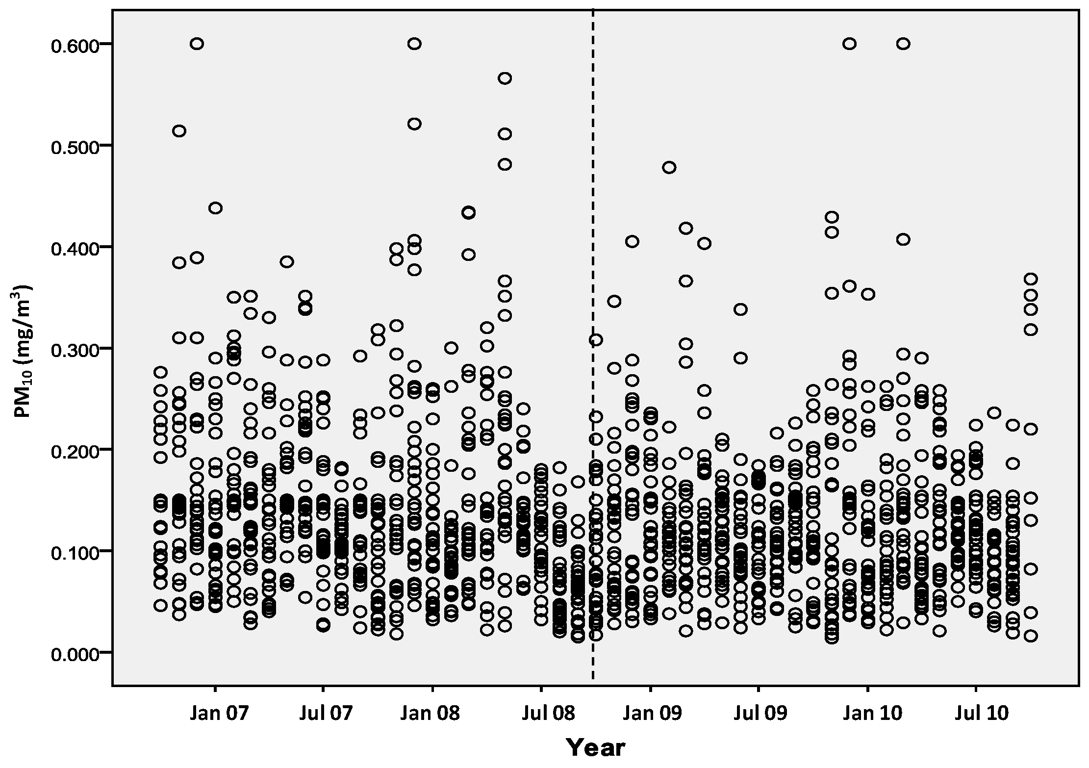
Figure 2.
Growth trends of motor vehicles in Beijing during 2004-2010.
| API Values | Concentrations of Pollutants (μg/m3, Daily Average) | Air Pollution Level | ||
|---|---|---|---|---|
| PM10 | SO2 | NO2 | ||
| 50 | 50 | 50 | 80 | Excellent |
| 100 | 150 | 150 | 120 | Good |
| 200 | 350 | 800 | 280 | Slightly polluted |
| 300 | 420 | 1600 | 565 | Moderately polluted |
| 400 | 500 | 2100 | 750 | Heavily Polluted |
| 500 | 600 | 2620 | 940 | Heavily Polluted |
| API | Air Pollution Level | 2007 | 2008 | 2009 | 2010 | Total | Health Effects [9] |
|---|---|---|---|---|---|---|---|
| 0–50 | I | 8.8% | 15.8% | 12.6% | 13.2% | 12.6% | Daily activity will not be affected. |
| 51–100 | II | 58.6% | 56.8% | 59.5% | 61.1% | 59.0% | Daily activity will not be affected. |
| 101–200 | III | 29.6% | 24.9% | 25.5% | 23.0% | 25.7% | The symptoms of the susceptible are slightly aggravated, while healthy people will have stimulated symptoms. |
| 201–300 | IV | 2.2% | 1.1% | 1.6% | 2.2% | 1.8% | Symptoms of the patients with cardiac and lung diseases will be aggravated remarkably. Healthy people will experience a drop in endurance and increased symptoms. |
| >300 | V | 0.8% | 1.4% | 0.8% | 0.5% | 0.9% | Exercise endurance of healthy people decreases. Some will have strong symptoms. Some diseases will appear. |
Table 3.
Estimates of the monthly effects of the 20% driving restriction on air quality in Beijing during the 4-year time window.
| Variables | (0) | (1) | (2) | (3) | (4) | (5) | (6) | (7) | (8) | (9) | (10) | (11) | (12) | (13) |
|---|---|---|---|---|---|---|---|---|---|---|---|---|---|---|
| 20% restriction | –0.007 (0.029) | –0.006 (0.031) | 0.006 (0.034) | 0.003 (0.039) | 0.000 (0.042) | 0.011 (0.049) | 0.028 (0.075) | 0.170 * (0.091) | 0.210 ** (0.091) | 0.238 *** (0.092) | 0.267 *** (0.092) | 0.275 *** (0.093) | 0.265 *** (0.094) | 0.258 *** (0.094) |
| 20% restriction adjustment | 0.040 * (0.024) | 0.039 (0.025) | 0.030 (0.027) | 0.032 (0.030) | 0.036 (0.034) | 0.025 (0.042) | 0.008 (0.069) | –0.117 (0.083) | –0.117 (0.083) | –0.116 (0.083) | –0.116 (0.083) | –0.116 (0.083) | –0.116 (0.083) | –0.117 (0.083) |
| MONTH 1 | –0.001 (0.058) | –0.013 (0.060) | –0.011 (0.063) | –0.007 (0.065) | –0.018 (0.069) | –0.035 (0.089) | –0.166 (0.101) | –0.185 * (0.101) | –0.199 ** (0.101) | –0.215 ** (0.101) | –0.219 ** (0.101) | –0.214 ** (0.101) | –0.200 * (0.103) | |
| MONTH 2 | –0.050 (0.054) | –0.048 (0.057) | –0.044 (0.059) | –0.055 (0.064) | –0.072 (0.084) | –0.202 ** (0.097) | –0.219 ** (0.097) | –0.232 ** (0.097) | –0.245 ** (0.097) | –0.249 ** (0.097) | –0.244 ** (0.097) | –0.242 ** (0.097) | ||
| MONTH 3 | 0.007 (0.057) | 0.010 (0.059) | 0.000 (0.064) | –0.018 (0.085) | –0.147 (0.097) | –0.162 * (0.097) | –0.174 * (0.096) | –0.188 * (0.097) | –0.191 ** (0.097) | –0.187 * (0.097) | –0.185 * (0.097) | |||
| MONTH 4 | 0.013 (0.055) | –0.003 (0.060) | –0.014 (0.082) | –0.155 (0.097) | –0.179* (0.097) | –0.193 ** (0.097) | –0.206 ** (0.097) | –0.209 ** (0.097) | –0.204 ** (0.097) | –0.198 ** (0.098) | ||||
| MONTH 5 | –0.028 (0.062) | –0.045 (0.084) | –0.184 * (0.098) | –0.207 ** (0.098) | –0.220 ** (0.098) | –0.233 ** (0.098) | –0.237 ** (0.098) | –0.231 ** (0.098) | –0.226 ** (0.098) | |||||
| MONTH 6 | –0.025 (0.082) | –0.165 * (0.097) | –0.189 * (0.097) | –0.204 ** (0.097) | –0.217 ** (0.097) | –0.221 ** (0.097) | –0.215 ** (0.097) | –0.209 ** (0.097) | ||||||
| MONTH 7 | –0.164 *** (0.060) | –0.188 *** (0.060) | –0.203 *** (0.061) | –0.215 *** (0.061) | –0.219 *** (0.061) | –0.213 *** (0.061) | –0.207 *** (0.062) | |||||||
| MONTH 8 | –0.191 *** (0.049) | −0.201 *** (0.049) | –0.213 *** (0.049) | –0.217 *** (0.049) | –0.211 *** (0.050) | –0.206 *** (0.050) | ||||||||
| MONTH 9 | –0.122 ** (0.049) | –0.134 *** (0.049) | –0.138 *** (0.049) | –0.133 *** (0.049) | –0.128 ** (0.050) | |||||||||
| MONTH 10 | –0.110 ** (0.049) | –0.114 ** (0.049) | –0.108 ** (0.049) | –0.105 ** (0.050) | ||||||||||
| MONTH 11 | –0.038 (0.049) | –0.032 (0.050) | –0.029 (0.050) | |||||||||||
| MONTH 12 | 0.040 (0.050) | 0.044 (0.051) | ||||||||||||
| MONTH 13 | 0.039 (0.051) | |||||||||||||
| Adj. R2 | 0.316 | 0.316 | 0.316 | 0.315 | 0.315 | 0.314 | 0.314 | 0.317 | 0.324 | 0.326 | 0.328 | 0.328 | 0.328 | 0.328 |
| Observations | 1461 | 1461 | 1461 | 1461 | 1461 | 1461 | 1461 | 1461 | 1461 | 1461 | 1461 | 1461 | 1461 | 1461 |
Notes: This table reports 14 regressions. For all regressions, the dependent variables are the daily city-level PM10 concentrations in logs. 20% restriction is the dummy of 20% driving restriction policy, 1 = after the implementation of the policy since 10/11/2008, 0 = before the implementation date. 20% restriction adjustment is the dummy of the adjusted 20% driving restriction policy since 11 April 2009. MONTH 1–MONTH 13 are monthly dummies indicating months after policy implementation, e.g., for Month 1, 1 = the 1st month after implementation, 0 = others. All regressions control for weather covariates (temperature, humidity, precipitation, wind speed and wind direction), month of the year, weekday dummy, odd-even dummy, and a linear time trend. Standard error is in parenthesis. Levels of significance are reported as * p < 0.10, ** p < 0.05, and *** p < 0.01.
| Variables | 4–year (October 2006–October 2010) | 3–Year (April 2007–April 2010) | 2–Year (October 2007–October 2009) | |||||||||
|---|---|---|---|---|---|---|---|---|---|---|---|---|
| OLS | (1) | (2) | (3) | OLS | (1) | (2) | (3) | OLS | (1) | (2) | (3) | |
| 20% restriction | 0.112 (0.084) | 0.258 *** (0.094) | 0.265 ** (0.114) | 0.291 ** (0.124) | 0.176 ** (0.087) | 0.355 *** (0.094) | 0.313 (0.193) | 0.521 ** (0.124) | 0.223 (0.242) | 0.475 * (0.255) | 0.581 ** (0.269) | 0.722 ** (0.293) |
| 20% restriction adjustment | –0.116 (0.083) | –0.117 (0.083) | –0.117 (0.083) | –0.117 (0.083) | –0.115 (0.084) | –0.115 (0.083) | –0.115 (0.083) | –0.116 (0.083) | –0.131 (0.082) | –0.132 (0.081) | –0.132 (0.081) | –0.132 (0.081) |
| MONTH 1 | –0.114 (0.100) | –0.200 * (0.103) | –0.206 * (0.120) | –0.223 * (0.125) | –0.117 (0.106) | –0.219 * (0.112) | –0.199 (0.184) | –0.312 * (0.186) | –0.251 (0.250) | –0.334 (0.250) | –0.439 * (0.256) | –0.581 ** (0.272) |
| MONTH 2 | –0.180 * (0.096) | –0.242 ** (0.097) | –0.246 ** (0.109) | –0.262 ** (0.113) | –0.209 ** (0.099) | –0.292 *** (0.103) | –0.276 * (0.159) | –0.357 ** (0.160) | –0.262 (0.249) | –0.264 (0.247) | –0.356 (0.249) | –0.484 * (0.258) |
| MONTH 3 | –0.121 (0.095) | –0.185 * (0.097) | –0.190 * (0.109) | –0.204 * (0.112) | –0.166 * (0.098) | –0.254 ** (0.103) | –0.237 (0.159) | –0.292 * (0.159) | –0.224 (0.248) | –0.224 (0.247) | –0.303 (0.248) | –0.417 (0.255) |
| MONTH 4 | –0.147 (0.097) | –0.198 ** (0.098) | –0.202 * (0.106) | –0.212 ** (0.107) | –0.135 (0.100) | –0.196 * (0.102) | –0.180 (0.154) | –0.234 (0.154) | –0.181 (0.249) | –0.184 (0.247) | –0.250 (0.249) | –0.349 (0.254) |
| MONTH 5 | –0.173 * (0.098) | –0.226 ** (0.098) | –0.230 ** (0.106) | –0.238 ** (0.107) | –0.149 (0.101) | –0.216 ** (0.103) | –0.200 (0.156) | –0.227 (0.155) | –0.230 (0.249) | –0.235 (0.248) | –0.288 (0.249) | –0.369 (0.252) |
| MONTH 6 | –0.159 (0.097) | –0.209 ** (0.097) | –0.212 ** (0.105) | –0.218 ** (0.105) | –0.194 * (0.099) | –0.257 ** (0.102) | –0.241 (0.154) | –0.246 (0.153) | –0.237 (0.249) | –0.240 (0.247) | –0.279 (0.248) | –0.342 (0.250) |
| MONTH 7 | –0.157 *** (0.060) | –0.207 *** (0.062) | –0.211 *** (0.072) | –0.215 *** (0.073) | –0.186 *** (0.065) | –0.226 *** (0.066) | –0.211 (0.129) | –0.249 * (0.128) | –0.161 (0.237) | –0.162 (0.236) | –0.188 (0.236) | –0.232 (0.237) |
| MONTH 8 | –0.155 *** (0.048) | –0.206 *** (0.050) | –0.210 *** (0.062) | –0.213 *** (0.063) | –0.240 *** (0.055) | –0.275 *** (0.056) | –0.262 ** (0.112) | –0.299 *** (0.111) | –0.277 (0.228) | –0.279 (0.227) | –0.292 (0.227) | –0.315 (0.227) |
| MONTH 9 | –0.076 (0.047) | –0.128 ** (0.050) | –0.132 ** (0.062) | –0.133 ** (0.062) | –0.150 *** (0.055) | –0.185 *** (0.056) | –0.173 * (0.103) | –0.191 * (0.102) | –0.099 (0.221) | –0.098 (0.220) | –0.098 (0.220) | –0.098 (0.220) |
| MONTH 10 | –0.052 (0.047) | –0.105 ** (0.050) | –0.108 * (0.062) | –0.108 * (0.062) | –0.111 ** (0.056) | –0.140 ** (0.057) | –0.130 (0.098) | –0.124 (0.097) | –0.061 (0.236) | –0.062 (0.235) | –0.049 (0.235) | –0.025 (0.235) |
| MONTH 11 | 0.014 (0.048) | –0.029 (0.050) | –0.033 (0.062) | –0.029 (0.063) | –0.044 (0.059) | –0.053 (0.059) | –0.044 (0.089) | –0.014 (0.089) | 0.130 (0.242) | 0.127 (0.241) | 0.154 (0.241) | 0.203 (0.242) |
| MONTH 12 | 0.090* (0.049) | 0.044 (0.051) | 0.041 (0.061) | 0.045 (0.061) | 0.049 (0.057) | 0.032 (0.057) | 0.040 (0.081) | 0.052 (0.081) | 0.194 (0.238) | 0.192 (0.237) | 0.232 (0.237) | 0.307 (0.240) |
| MONTH 13 | 0.059 (0.051) | 0.039 (0.051) | 0.036 (0.058) | 0.037 (0.058) | 0.086 (0.060) | 0.075 (0.059) | 0.081 (0.074) | 0.096 (0.074) | –0.204 (0.242) | –0.037 (0.247) | 0.015 (0.252) | 0.118 (0.264) |
| Adj. R2 | 0.323 | 0.328 | 0.327 | 0.327 | 0.327 | 0.331 | 0.330 | 0.337 | 0.361 | 0.368 | 0.368 | 0.368 |
| Observations | 1461 | 1461 | 1461 | 1461 | 1096 | 1096 | 1096 | 1096 | 731 | 731 | 731 | 731 |
Notes: This table reports 12 regressions control for different polynomial orders during different time windows. For all regressions, the dependent variables are the daily city-level PM10 concentrations in logs. 20% restriction and 20% restriction adjustment are the dummies of the 20% driving restriction and the adjusted 20% driving restriction policy, respectively. MONTH 1–MONTH 13 are monthly dummies indicating months after policy implementation. All regressions control for weather covariates, month of the year, weekday dummy, and odd-even dummy. Standard error is in parenthesis. Levels of significance are reported as * p < 0.10, ** p < 0.05, and *** p < 0.01.
© 2016 by the authors; licensee MDPI, Basel, Switzerland. This article is an open access article distributed under the terms and conditions of the Creative Commons Attribution (CC-BY) license (http://creativecommons.org/licenses/by/4.0/).
Share and Cite
MDPI and ACS Style
Ma, H.; He, G. Effects of the Post-Olympics Driving Restrictions on Air Quality in Beijing. Sustainability 2016, 8, 902. https://doi.org/10.3390/su8090902
AMA Style
Ma H, He G. Effects of the Post-Olympics Driving Restrictions on Air Quality in Beijing. Sustainability. 2016; 8(9):902. https://doi.org/10.3390/su8090902
Chicago/Turabian StyleMa, Hua, and Guizhen He. 2016. "Effects of the Post-Olympics Driving Restrictions on Air Quality in Beijing" Sustainability 8, no. 9: 902. https://doi.org/10.3390/su8090902
Note that from the first issue of 2016, this journal uses article numbers instead of page numbers. See further details here.