A Grey Forecasting Approach for the Sustainability Performance of Logistics Companies

Abstract

Logistics plays an important role in globalized companies and contributes to the development of foreign trade. A large number of external conditions, such as recession and inflation, affect logistics. Therefore, managers should find ways to improve operational performance, enabling them to increase efficiency while considering environmental sustainability due to the industry’s large scale of energy consumption. Based on data collected from the financial reports of top global logistics companies, this study uses a DEA model to calculate corporate efficiency by implementing a Grey forecasting approach to forecast future sustainability values. Consequently, the study addresses the problem of how to enhance operational performance while accounting for the impact of external conditions. This research can help logistics companies develop operation strategies in the future that will enhance their competitiveness vis-à-vis rivals in a time of global economic volatility.

1. Introduction

In this era of global competition, international trade has played an important role in developing companies. For these countries, the provision of efficient transport infrastructure is critical to support businesses in their efforts to contribute to sustainable development through their core business activities. Key activities are those that physically connect a business to its supply chain partners [1]. However, logistics connectivity can work as a driving force with regard to economic growth, not only by facilitating the achievement of environmental targets, such as reducing emissions, but also by supporting applied technology as a major factor that can help meet sustainable development goals. These technology-related targets can be separated into three categories: (a) significant overall technology performance improvement; (b) universal access to sustainable technology; and (c) an effective global innovation system for sustainable development [2]. Technology can help build on synergies among these goals, realize possible multiple benefits and avoid barriers and conflicts. Strengthening national systems of innovation to accelerate technology progress in industrial logistics is very important. If logistics connectivity is not fully integrated into sustainability goals, companies will fall behind the global competition, and logistics connectivity failures could decrease the likelihood of growth through trade.

Logistics investments not only link producers and consumers to create more productive divisions, but also provide a key supply chain component that ensures the efficient movement and timely availability of raw materials and finished products [3]. One major challenge is that customers have become smarter in their choices and tend to expect low-cost, high-quality service, as well as fast transportation timing, while the targets include reducing environmental emissions. Fortunately, one of the potential solutions is the prediction of future developments in the shipping and logistics industry. Predicting a future development is a fundamental and important pursuit in many fields, including economics, physics and engineering.

To obtain a reliable prediction, certain laws governing the phenomena of system development must be understood through either natural principles or real observations [4,5]. Especially for logistics companies, which operate in the field of transportation, forecasting the demand for transportation plays a very important role. Accurate prediction helps companies allocate their investments properly, meet demands for transportation, manage future income and costs, solve supply chain problems and improve competitive advantages.

One of the biggest difficulties that businesses commonly face is the high cost of equipment investment, transportation and fuel resources. Another difficulty is that the final outputs of a transportation company, such as income revenue and relative costs, must be evaluated as a basis of the proposed business plan for the following year. Transportation businesses, however, often pay little attention to the prediction of these financial measures. Failing to make accurate predictions increases the risk for businesses and causes them to miss opportunities that the market offers. What, then, are the criteria commonly used to evaluate business operations and forecast future operation activities? Considering this question, the authors were motivated to examine the topic with the aim of helping transportation companies improve their performance evaluations and implementation of forecasting. The results of this study can help businesses improve their competitiveness in the international market.

2. Theoretical Foundation

2.1. Performance Management

Performance management is the process of improving the performance of organizations, teams and individuals, driven by line managers [6]. Organizational performance has always exerted considerable influence on the actions of the dynamic market [7]. Consequently, performance management is recognized as an important part of the literature on manufacturing strategy. Nowadays, performance management is evolving rapidly to a comprehensive framework of sustainability criteria that focus on operational practices in the manufacturing sector and, more specifically, the assessment of the sustainability performances of technological developments during performance management. The concept of performance, as it is measured and evaluated, is undergoing a transformation in modern business organizations and in business operations groups. Performance management is the use of performance measurement information to effectively and positively change organizational culture, systems and processes, by helping to establish agreed-upon performance goals, allocating and prioritizing resources, advising managers to either confirm or change current policy or programmed directions to meet goals and sharing the results of performance. The most modern and dynamic industries are transnational, because they are the result of an integrated system of global trade and performance. Therefore, there is a need to ensure logistics connectivity, especially to developing countries, which will depend significantly on the level of connectivity such countries have underdeveloped in their logistics networks. Performance management emphasizes more focus on enhancing logistics connectivity in conjunction with greater trade facilitation by interconnecting all modes of transport to offer seamless travel, better lead times, less congestion, more job opportunities, greater movement of goods and an economic stimulus package. To curtail logistics activity, there will be a need to highlight the immense benefits of investing in sustainable logistics growth, which will bring forth the right combination of economic and environmental benefits [8].

Sustainability in performance management is a market leading practice that helps customers define and implement management strategies that create measurable improvements in sustainability and business performance in logistics. Some companies did not have extensive experience implementing sustainability performance management programs from strategy definition all the way through deployment and operations. Thus, many companies are starting to develop a more strategic approach to sustainability performance management. According to Searcy 2012, corporate sustainability performance measurement must address issues associated with the “triple bottom line” of economic, environmental and social performance. Thus, measurement sustainability is defined as a system of indicators that provides a corporation with information needed to help in the short- and long-term management, controlling, planning and performance of the economic, environmental and social activities undertaken by the corporation [2]. That, in turn, means that sustainability data can truly help management understand the levers that most influence business performance in the logistics process. The net result of this full-fledged sustainability performance management is that sustainability becomes an integral part of strategic planning.

2.2. Related Research about GM (1,1)

In industrial logistics, forecasting is an important determinant of operational performance, although there have been few studies that have selected forecasting methods on that basis. A dynamic grey forecasting method is proposed in this paper to improve forecasting accuracy. The grey system theory, established by Deng in 1982, is a new methodology that focuses on the study of problems involving small samples and poor information [9]. Grey model forecasting GM (1,N) is the most widely-used central model, and discrete Grey models are a class of new models we initially developed. Grey theory is a truly multidisciplinary and generic theory dealing with systems that are characterized by poor information and/or a lack of information. The fields covered by Grey theory include systems analysis, data processing, modeling, prediction, decision-making and control. Grey forecasting models have been extensively used in many applications. The GM (1,1) is one of the most frequently used grey forecasting models. GM (1,N), proposed by Ren (2013), proved that using a grey model to predict the yield of biohydrogen under scanty data conditions could give a better predictability result than an artificial neural network approach [10]. Li [1] applied GM (1,1) to forecast electricity consumption effectively in the short term for Asian countries with a limited sample size. This model is a time series-forecasting model, encompassing a group of differential equations adapted for parameter variance, rather than a first order differential equation. Its difference equations have structures that vary with time rather than being general difference equations. Consequently, grey forecasting is a good tool for forecasting the values of the future mutual relationship among these factors based on a small amount of data. In this research, the authors applied a Grey model to forecast sustainability performance using past data to accurately simulate future performance results. A new vision inside and outside of corporate sustainability has also been researched, relating to the competitiveness business process for improving long-term economic performance. Supporting motivations could include improved image and reputation, cost savings, improved performance, improved competitiveness and reduced risk, among others.

2.3. Related Research about DEA

In this paper, a sustainability management performance evaluation methodology based on DEA has been proposed as a non-parametric technique to measure the relative efficiency of firms, which can incorporate multiple inputs and outputs at multiple stages and which results in a single relative efficiency measure. Data envelopment analysis (DEA) is a nonparametric programming technique used to treat problems of multiple inputs and outputs associated with multiple decision-making units (DMUs). The DEA is used to establish a best practice group from among a set of observed units and to identify the units that are inefficient when compared to the best practice group [11]. Thus, for measuring sustainability, the most important advantages of DEA are that (a) it provides clear and obvious standardization, ranking all units using a score from zero (worst performance) to one (best performance) and (b) it allows economic data to be quantified and linked to business performance if the case for sustainability is to be made and the benefits are to be realized; these weights are defined by the DEA procedure in the computation of efficiency. Because conventional DEA models are found to be ineffective in measuring the performance of various transport-related functions, many multi-stage DEA models have been developed to account for various indirect processes and their contribution to corporate performance. In the logistics industry, competitors are continuously struggling to differentiate themselves from other companies in the market. Performance, as we have stated above, is about the future. The budget process is about evaluating and selecting possible action plans that will help the firm achieve customer satisfaction in the future.

DEA is an approach for sustainability measuring the relative efficiency of a “data-oriented” approach for evaluating the performance of a set of peer entities called DMUs with multiple inputs and multiple outputs, using mathematical programming. Additionally, the DEA has been recognized as an excellent method for analyzing performance, modeling organizations and evaluating operational processes, particularly when market prices are unavailable [12]. Techniques developed to measure efficiency require the estimation of a production frontier against which a firm’s performance may be evaluated in developing sustainable industrial logistics. Non-parametric techniques do not specify the functional form of the frontier. Instead, these techniques establish a set of segments linking efficient firms, which combine environmental efficiency comparing the rest of the units. The main interest here is for choosing the DEA is that the technique does not predefine any functional form for the production function and then, efficiency evaluation were designed to analyse industries comprising multi-input multi-output producers in order to measure its contribution to productivity [13,14]. In addition, it is not financially oriented in principle; instead, the objective is to perform an analysis of the process of the transformation of inputs into outputs that generates a measurement or set of measurements, which reflects the efficiency of a firm with regard to the transformation process. The DEA has an additional advantage because it can incorporate any number of inputs and outputs into the analysis. Further, these inputs and outputs can be of any nature; the only requirement is the availability of a unit of measurement to assess its magnitude.

Some prior research constructed an efficient evaluation for a shipping industry with financial indicators to evaluate performance [15]. Emmanuel [14] used DEA to evaluate efficiency in the education sector, which comprises multi-input, multi-output producers and lacking data. The DEA method is also widely applied to analyze sustainability in the energy field; the DEA approach was proposed by Ren to analyze sustainability efficiencies of biodiesel production systems, including soybean, rapeseed, sunflower, jatropha and palm-based diesel production [11]. Ren [16] indicated that DEA was a novel and feasible method for finding efficient bioethanol production scenarios. According to Soteriou [17], DEA was an effective model for bank branch performance assessment in terms of internal customer service quality. The main purpose of this research was to measure the operating efficiency of sustainable industrial logistics. We hence propose a performance evaluation methodology based on DEA, which can incorporate multiple inputs and outputs in multiple stages and which will result in a single relative efficiency measure. DEA has not been used to compare subunits within a given transit organization. Herein, we demonstrate the use of DEA for comparing a set of subunits that each performs the same activity within its parent transportation agency [12,18]. Applying technological innovation is an important way for enterprises to obtain sustainable competitive advantage [19]. The Malmquist productivity index can be decomposed into two components measuring the change in the technology frontier and technical efficiency (catch-up). Instead, these techniques establish a set of segments linking efficient firms, which is combined environmental efficiency comparing the rest of the units. In this paper, we further examine the two components to reveal sources and patterns of productivity change that are obscured by the aggregated nature of the Malmquist index. It is shown that more information can be derived from the individual Malmquist components. Our proposed new approach not only reveals patterns of productivity change and presents a new interpretation along with the managerial implication of each Malmquist component, but also identifies the strategy shifts of individual DMUs in a particular time period. We can make judgments regarding whether such strategy shifts are favorable and promising. The “strategy shift” here is characterized by changes in the isoquant. The next section reviews how the DEA-based Malmquist productivity index works. We then present our new Malmquist productivity approach in line with the profit-maximizing objective of the logistics companies by measuring sustainability-oriented performance. Because it is the logistics companies who decide on the level of inputs, a decrease in input levels resulting in an increase of technology in sustainability performance management should be profitable to achieve sustainable, environmentally-friendly industrial logistics.

2.4. Collecting the Data of Logistics Companies

Armstrong & Associates, Inc., examined the top 25 logistics companies in the world [20]. Primarily, this study is based on public financial reports published by GuruFocus.com [21], which is engaged in the business of financial news, commentaries, research and publishing. This website contained the stock picks and portfolios of the world’s best investors. We eliminated incomplete data with missing information, such as certain information in the year 2015 and certain data regarding shipping logistics in 19 companies from Europe, Japan, America and Korea.

3. Methodology

3.1. Grey Forecasting Generation Theory

GM (1,1) is the central model that has been most widely employed, and discrete grey models are a class of new models we initially developed [22].

Let $X^{\left(0\right)}=\left(x^{\left(0\right)}\right(1),x^{\left(0\right)}(2),\dots ,x^{\left(0\right)}(n\left)\right)$be a sequence of raw data. Denote its accumulation-generated sequence by $X^{\left(1\right)}=\left(x^{\left(1\right)}\right(1),x^{\left(1\right)}(2),\dots ,x^{\left(1\right)}(n\left)\right)$. Then, $X^{\left(0\right)}\left(k\right)+a{x}^{\left(1\right)}\left(k\right)=b$ is referred to as the original form of the GM (1,1) model, where the symbol GM (1,1) stands for “first order grey model in one variable”.

Let $Z^{\left(1\right)}=\left(z^{\left(1\right)}\right(1),z^{\left(1\right)}(2),\dots ,z^{\left(1\right)}(n\left)\right)$ be the sequence generated from $X^{\left(1\right)}$ by the adjacent neighbor means; that is, $z^{\left(1\right)}\left(k\right)=\frac{1}{2}\left(x^{\left(1\right)}\right(k)+x^{\left(1\right)}(k-1\left)\right),k=2,3,\dots ,n.$ Then, $x^{\left(0\right)}\left(k\right)+a{z}^{\left(1\right)}\left(k\right)=b\left(1\right)$ is referred to as the basic form of the GM (1,1) model.

Theorem: Let $X^{\left(0\right)}$, $X^{\left(1\right)}$, and $Z^{\left(1\right)}$ be the same as the above, except that $X^{\left(0\right)}$ is non-negative. If $\widehat{a}={(a,b)}^T$ is the sequence of parameters:

$$Y=\left[\begin{array}{c}{x}^{\left(0\right)}\left(2\right)\\ x^{\left(0\right)}\left(3\right)\\ ⋮\\ x^{\left(0\right)}\left(n\right)\end{array}\right],B=\left[\begin{array}{c}\begin{array}{cc}-z^{\left(1\right)}\left(2\right)& 1\end{array}\\ \begin{array}{cc}-z^{\left(1\right)}\left(3\right)& 1\end{array}\\ \begin{array}{cc}⋮& 1\end{array}\\ \begin{array}{cc}-z^{\left(1\right)}\left(n\right)& 1\end{array}\end{array}\right]$$

The least squares estimate sequence of the GM (1,1) model satisfies $\widehat{a}={\left(B^{T}B\right)}^{-1}{B}^{T}Y$ [1]. Continuing all of the notations from Theorem 1, if ${[a,b]}^T={\left(B^{T}B\right)}^{-1}{B}^{T}Y$, then $\frac{d{x}^{\left(1\right)}}{dt}+a{x}^{\left(1\right)}=b$ is a whitenization equation of the GM (1,1).The time response sequence of the GM (1,1) is given below.

$${\widehat{x}}^{\left(1\right)}(k+1)=\left(x^{\left(0\right)}(1)-\frac{b}{a}\right)e^{-ak}+\frac{b}{a},k=1,2,\dots ,n$$

The parameters $(-a)$ and $b$ of GM (1,1) are referred to as the development coefficient and Grey action quantity, respectively. The former reflects the development states of ${\widehat{x}}^{\left(1\right)}$ and ${\widehat{x}}^{\left(0\right)}$ [22]. In general, the variables that act upon the system of interest should be external or pre-defined. Because GM (1,1) is a model constructed on a single sequence, it uses only the behavioral sequence (referred to as the output sequence or background values) of the system without considering any externally-acting sequences (referred to as input sequences or driving quantities). The Grey action quantity in GM (1,1) is a value derived from the background values. It reflects changes contained in the data, and its exact intension is grey. This quantity realizes the extension of the relevant intension. Its existence distinguishes grey systems modeling from the general input-output modeling. It is also an important test of the conclusions of grey systems and grey boxes.

3.2. Valuation Performances

Regarding the evaluation performance of the volatility model for forecasting, there are some common approaches, including the root of mean square error (RMSE), mean absolute error (MSE), and mean absolute percentage error (MAPE). This paper uses MAPE to identify the Grey prediction models with good performance; a small MAPE is defined as follows:

$$MAPE=\frac{1}{n}{\displaystyle \sum }_{k=2}^n\left|\frac{x^{\left(0\right)}(k)-{\widehat{x}}^{\left(0\right)}(k)}{x^{\left(0\right)}\left(k\right)}\right|\times 100\%$$

where: $x^{\left(0\right)}(k)$ = the actual value in time period k. ${\widehat{x}}^{\left(0\right)}(k)$ = the forecast value in time period k.

The grades of MAPE are divided into four levels, as shown in

Table 1. The grades of MAPE.

MAPE	≤10%	10%–20%	20%–50%	>50%
Grade levels	Excellent	Good	Qualified	Unqualified

.

3.3. Malmquist Productivity Index

The Malmquist productivity index (MPI) was introduced by Caves in 1982 [23]. The researchers expanded upon an idea of Malmquist (1953), who in a consumer context used ratios of input distance functions to construct an input quantity index. Färe et al. [24] followed and developed the work of Caves, Christensen and Diewert. They calculated an adjacent Malmquist productivity index consisting of the geometric mean of two Malmquist indexes as defined by Caves, Christensen and Diewert. Later, Berg introduced a base period Malmquist productivity index, which (except for the fixed base period technology) is the same as one of the indexes defined by Caves [23]. Consequently, they argue that one desirable property of an index covering a longer period of time is the possibility to chain it; the index obeys the circular relation, and the price we must pay for the fulfillment of the circular test seems reasonable [12]. If we use the base period Malmquist productivity index instead of the adjacent index, we fulfill the circular test, but pay with base period dependency and with an underlying reference to a fixed technology that might have nothing in common with the technologies of the two periods under consideration.

Productivity measurement was an important research topic, and DEA introduced a useful approach; productivity measurement in DEA was the Malmquist productivity index (MPI), which was named after Malmquist, to give ideas for the MPI [6]. In addition, other scholars assumed that Malmquist calculates the relative performance of a DMU in different periods of time using the technology of the base period [24].

In this research, we adopted the theorem of Chen (2003) [25] and selected n $DM{U}_s$; each $DM{U}_j(j=1,2,\dots ,n)$produces a vector of outputs$y_j^t=(y_{1j}^t,\dots ,y_{sj}^t)$ by using a vector of inputs $x_j^t=(x_{1j}^t,\dots ,x)$ at each time period$t,t=1,\dots ,$ t, which could be the CCR (Chames, Cooper and Rhodes) DEA model as: ${\theta }_0^t(x_0^t,y_0^t)=mi{n}_{{\theta }_0,{\lambda }_j}{\theta }_0$, s.t ${\sum }_{j=1}^n{\lambda }_j{x}_j^t\le {\theta }_0{x}_0^t$, ${\sum }_{j=1}^n{\lambda }_j{x}_j^t\ge y_0^t$${\lambda }_j\ge 0,j=1,\dots ,n$, where $x_0^t=(x_{10}^1,\dots ,x_{m0}^t)$ and $y_0^t=(y_{10}^1,\dots ,y_{s0}^t)$ means input and output vectors of $DM{U}_0$, among others. Theorem is shown to be input-oriented, because it acknowledges that the possible redial reductions of all inputs are fixed at current levels of the company [12].

If ${\theta }_0^t(x_0^t,y_0^t)=1$, then $DM{U}_0$ is (radially) efficient in time period $t$; otherwise, if ${\theta }_0^t(x_0^t,y_0^t)<1$, then $DM{U}_0$ is (radially) invalid. We observe that: (i) if ${\theta }_0^t(x_0^t,y_0^t)=1$, then $DM{U}_0$ is on the empirical production frontier (EPF); and (ii) if ${\theta }_0^t(x_0^t,y_0^t)<1$, then $DM{U}_0$ can reduce its inputs, and therefore, $DM{U}_0$ is operating below the EPF. Note that the possible non-zero input and output slacks are likely to present at the optimal solutions.

Replacing $x_j^t$ and $y_j^t$ with $x_j^{t+1}$ and $y_j^{t+1}$, respectively, we have the technical efficiency of ${\theta }_0^{t+1}(x_0^{t+1},y_0^{t+1})$ for $DM{U}_0$ at the time period $t+1$. From $t$to $t+1,DM{U}_0’s$ technical efficiency may change or the EPF may shift. Based on this model, the radial Malmquist productivity index can be calculated via [24].

(i)

Comparing $x_0^t$ to EPF at time t, calculating ${\theta }_0^t(x_0^t,y_0^t)$;

(ii)

Comparing $x_0^{t+1}$ to EPF at time t + 1, calculating ${\theta }_0^{t+1}(x_0^{t+1},y_0^{t+1})$ through the following linear program:

$${\theta }_0^{t+1}(x_0^t,y_0^t)=mi{n}_{{\theta }_0,{\lambda }_j};s.t{\sum }_{j=1}^n{\lambda }_j{x}_j^{t+1}\le {\theta }_0{x}_0^t;{\sum }_{j=1}^n{\lambda }_j{x}_j^{t+1}\ge y_0^{t+1}{\lambda }_j\ge 0,j=1,\dots ,n$$

The Malmquist productivity index is defined as $P{I}_0$:

$$P{I}_0={\left[\frac{{\theta }_0^t(x_0^t,y_0^t){\theta }_0^{t+1}(x_0^t,y_0^t)}{{\theta }_0^t(x_0^{t+1},y_0^{t+1}){\theta }_0^{t+1}(x_0^{t+1},y_0^{t+1})}\right]}^{\frac{1}{2}}$$

(1)

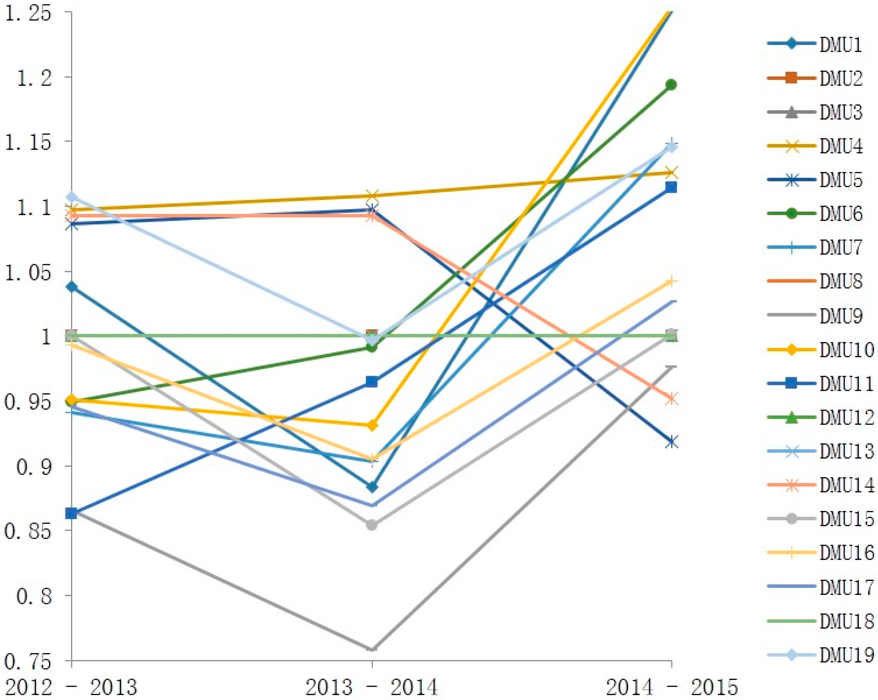
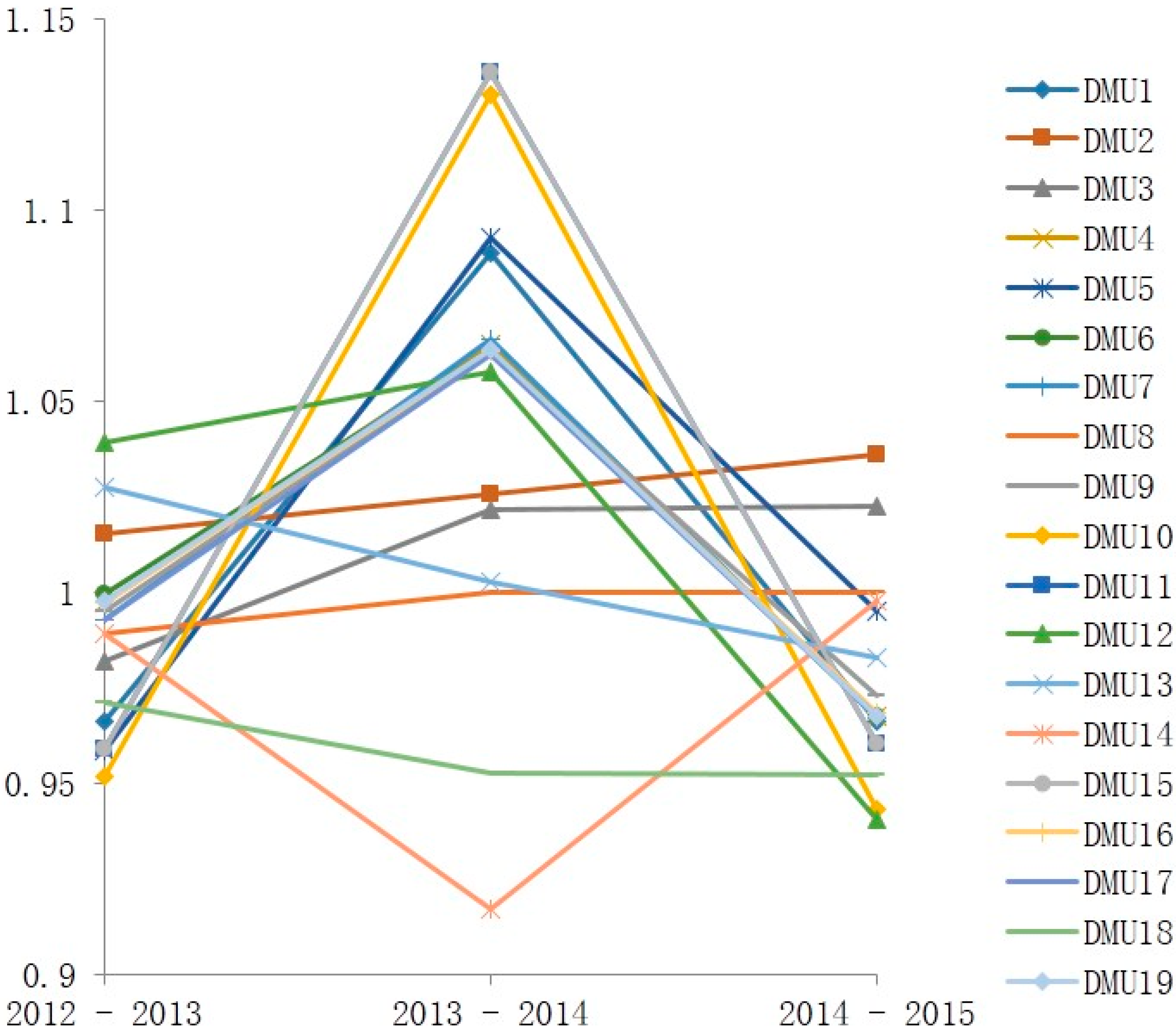
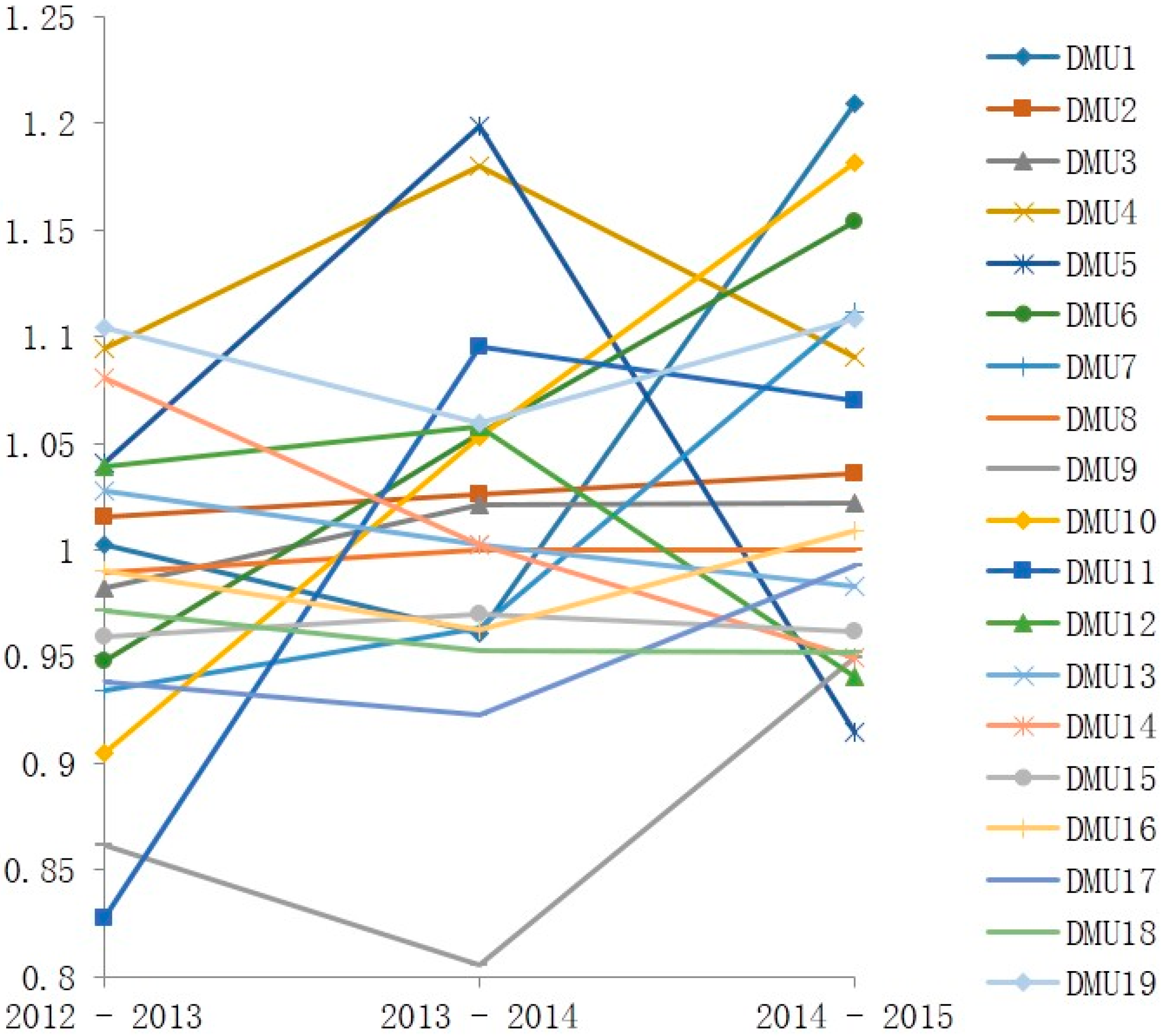
$P{I}_0$ measures the productivity change between periods $t$ and $t+1$. Productivity declines if $P{I}_0>1$, remains unchanged if $P{I}_0=1$ and improves if $P{I}_0<1$. Note that $P{I}_0$is expressed by the radial efficiency scores obtained from several input-oriented DEA models. Therefore, this $P{I}_0$ is called the input-oriented radial Malmquist productivity index.

The following modification of $P{I}_0$ makes it possible to measure the change in technical efficiency and the movement of EPF for $DM{U}_0$:

$$P{I}_0=\frac{{\theta }_0^t(x_0^t,y_0^t)}{{\theta }_0^{t+1}(x_0^{t+1},y_0^{t+1})}{\left[\frac{{\theta }_0^{t+1}(x_0^{t+1},y_0^{t+1})}{{\theta }_0^t(x_0^{t+1},y_0^{t+1})}\frac{{\theta }_0^{t+1}(x_0^t,y_0^t)}{{\theta }_0^t(x_0^t,y_0^t)}\right]}^{\frac{1}{2}}$$

The first term on the right-hand side measures the magnitude of technical efficiency change between period $t$ and $t+1$ and whether technical efficiency improves, remains or declines, accordingly. The second term measures the shift in the EPF between periods $t$ and $t+1$:

$$\frac{{\theta }_0^t(x_0^t,y_0^t)}{{\theta }_0^{t+1}(x_0^{t+1},y_0^{t+1})=1}$$

(2)

We should note the possibility that two different period EPFs may have intersections. The facets of EPF may not shift in the same direction; some facets may shift forward and some backward. In this situation, the movement of EPF is DMU-specific. The Malmquist productivity index measures the performance of a specific DMU in terms of the change or referent DMUs.

The selection of ${\alpha }_i$ is independent of the corresponding input units. Possible choices of ${\alpha }_i$ can be ${\alpha }_i=1/x_{i0}$ and ${\alpha }_i=x_{i0}/{\sum }_{j=1}^n{x}_{ij}$. However, if additional information (e.g., con ratios) is available, then the lower bounds on multipliers can be used as weights ${\alpha }_i$.

Furthermore, if $v_i=\frac{\alpha }{x_{i0}^t{\sum }_{i=1}^m{\alpha }_i}$ $i=1,\dots ,m$, then ${\sum }_{r=1}^s{u}_r{y}_{rj}^t\le A_j$ $j=1,\dots ,n$, where$A_j={\sum }_{i=1}^m\frac{{\alpha }_i}{x_{ij}^t{\sum }_{i=1}^m{\alpha }_i}$, which can be interpreted as the weighted output for $DM{U}_j$ at time period $t$. Thus, we may use ${\sum }_{i=1}^m\widehat{{\alpha }_i}{x}_{ij}^t$ to estimate un-normalized $\widehat{{\alpha }_i}$ given the information on $A_j$. $A_j$ can be obtained from additional information (e.g., the total expenditure for each $DMU$ in a particular time period or the prices on outputs).

3.4. Measuring Sustainability Performance

This study is concerned with the metrics that can accurately reflect sustainability performance in logistics, utilizing the intellectual cost of goods sold, selling, general and administrative, equity and current assets. The input variables adopted in this study are as follows: X1: cost of goods sold, selling, general and administrative [26,27]; X2: total equity [28]; X3: total current assets [29], Y1: net income [28], Y2: gross profit [23]; and Y3: operation income [23].

4. Results and Discussions

4.1. Results and Analysis of the Grey Forecasting of the Input and Output Values for Logistics Companies

The author used the GM (1,1) model to predict the realistic input/output values of the top 19 logistics companies from 2016–2019. The crisis escalates from a problem in a few geographically peripheral countries to a full-blown financial and sovereign debt crisis engulfing the core logistics industry from the previous years, due to companies’ focus on investing in business transportation goods. However, according to GM (1,1) forecasting and data, this article estimates the data value of logistics companies from 2012–2019. An explanation follows.

The sequence of raw data $X^{\left(0\right)}=\left(x^{\left(0\right)}\right(1),x^{\left(0\right)}(2),x^{\left(0\right)}(3),x^{\left(0\right)}(4\left)\right)=(11,779,12,619,13,399,14,197)$ simulates this sequence$X^{\left(0\right)}$ by respectively using the following three GM (1,1) and comparing the accuracy of the simulation:

From $x^{\left(0\right)}\left(k\right)+a{z}^{\left(1\right)}\left(k\right)=b$; compute the accumulation generation of $X^{\left(0\right)}$ as follows:

$$X^{\left(1\right)}=(x^{\left(1\right)}(1),x^{\left(1\right)}(2),x^{\left(1\right)}(3),x^{\left(1\right)}(4))=(11,779,12,979,13,616.78,14,896.275)$$

We check the quasi-smoothness. From ${\sigma }^{\left(1\right)}(k)=\frac{x^{\left(0\right)}(k)}{x^{\left(1\right)}(k-1)}$, it follows that ${\sigma }^{\left(1\right)}\left(2\right)$ = 0.972, ${\sigma }^{\left(1\right)}\left(3\right)$ = 0.984 and ${\sigma }^{\left(1\right)}\left(4\right)$= 0.953. Therefore, k > 3, ${\sigma }^{\left(1\right)}\left(k\right)\in (0.5,1]$ with $\sigma =0.9(\mathrm{i}.\mathrm{e}.$, the law of the quasi-exponential and the condition of quasi-smoothness is stratified). Thus, we can establish a GM (1,1) model for $X^{\left(1\right)}$. Using the adjacent neighbors of sequence, let $Z^{\left(1\right)}=\left(z^{\left(1\right)}\right(1),z^{\left(1\right)}(2),\dots ,z^{\left(1\right)}(n\left)\right)$ be the sequence generated from $X^{\left(1\right)}$ by the adjacent neighbor means sequence $Z^{\left(1\right)}=\left(z^{\left(1\right)}\right(2),z^{\left(1\right)}(3),z^{\left(1\right)}(3),z^{\left(1\right)}(4\left)\right)$ = (18,286.5, 31,566.4, 45,822.9).

In addition, matrix $B$ and constant vector $Y_N$ are accumulated as follows:

$$B=\left[\begin{array}{cc}-18,268.5& 1\\ -31,566.4& 1\\ -45,822.9& 1\end{array}\right]Y_N=\left[\begin{array}{c}12,979\\ 13,616\\ 14,896\end{array}\right]$$

By using the least squares estimation, we obtain the sequence of parameters$\widehat{a}={[a,b]}^T$ as follows $\widehat{a}={\left(B^{T}B\right)}^{-1}{B}^{T}Y=\left[\begin{array}{c}0.069\\ 11,604.3\end{array}\right]$. We establish the model $\frac{d{x}^{\left(1\right)}}{dt}-0.0698x^{\left(1\right)}=11,604.3$ and its time response form $\widehat{x}(k+1)=(x^{\left(0\right)}(1)-\frac{b}{a})e^{-a\left(k\right)}+\frac{b}{a}=(x^{\left(0\right)}(1)-\frac{11604.3}{(-0.0698)})e^{-\left(0.069\right)k}+\frac{11604.3}{(-0.0698)}$. We substitute different values of $k$ into the equation: $k=1X^{\left(1\right)}\left(1\right)=11,979$; $k=2X^{\left(1\right)}\left(2\right)=24,649.86$; $k=3X^{\left(1\right)}\left(3\right)=38,451.53$; $k=4X^{\left(1\right)}\left(4\right)=53,251.32$; $k=5X^{\left(1\right)}\left(5\right)=69,121.41$; $k=6X^{\left(1\right)}\left(6\right)=86,139.21$; $k=7X^{\left(1\right)}\left(7\right)$ = 104,387.71; $k=8X^{\left(1\right)}\left(8\right)=123,955.92$.

We compute the simulated values of $X^{\left(0\right)}$ in the original series according to the accumulated generating operation by using ${\widehat{x}}^{\left(0\right)}(k+1)={\alpha }^{\left(1\right)}{\widehat{x}}^{\left(1\right)}(k+1)-{\widehat{x}}^{\left(1\right)}(k)$:

• $X^{\left(0\right)}\left(1\right)=x^{\left(1\right)}\left(1\right)=11,979$—forecast of the year 2012
• $X^{\left(0\right)}\left(2\right)=x^{\left(1\right)}\left(2\right)-x^{\left(1\right)}\left(1\right)=12,870.86$—forecast of 2013
• $X^{\left(0\right)}\left(3\right)=x^{\left(1\right)}\left(3\right)-x^{\left(1\right)}\left(2\right)=13,801.67$—forecast of 2014
• $X^{\left(0\right)}\left(4\right)=x^{\left(1\right)}\left(4\right)-x^{\left(1\right)}\left(3\right)=14,799.78$—forecast of 2015
• $X^{\left(0\right)}\left(5\right)=x^{\left(1\right)}\left(5\right)-x^{\left(1\right)}\left(4\right)=15,870.09$—forecast of 2016
• $X^{\left(0\right)}\left(6\right)=x^{\left(1\right)}\left(6\right)-x^{\left(1\right)}\left(5\right)=17,017.79$—forecast of 2017
• $X^{\left(0\right)}\left(7\right)=x^{\left(1\right)}\left(7\right)-x^{\left(1\right)}\left(6\right)=18,248.5$—forecast of 2018
• $X^{\left(0\right)}\left(8\right)=x^{\left(1\right)}\left(8\right)-x^{\left(1\right)}\left(7\right)=19568.21$—forecast of 2019.

Implementing the above computation process, the study could calculate the forecasting input and output of all DMUs from 2016–2019. To measure the accuracy of our forecasting results, we calculate the mean absolute percent error (MAPE) of each DMU from 2012–2015 (see

Table 2. Average MAPEs of decision-making units (DMUs).

DMUs	Average MAPE (%)	DMUs	Average MAPE (%)
DMU1	0.9462	DMU11	1.4125
DMU2	0.7709	DMU12	1.227
DMU3	0.27	DMU13	0.6516
DMU4	1.2972	DMU14	2.742
DMU5	1.983	DMU15	0.384
DMU6	0.505	DMU16	0.469
DMU7	1.263	DMU17	1.083
DMU8	1.4853	DMU18	1.65
DMU9	2.662	DMU19	0.588
DMU10	3.0697
Average MAPE		1.2815%

); the average forecasting error is hence computed as 1.2815%.

The results shown in Table 2 indicate that the MAPE of DMU₃ is the lowest (0.27%), while the maximum MAPE is 3.0697% (DMU₁₀). According to Liu [30], if the average residual error is below 10%, the forecasting process is highly reliable. Table 1 shows that all 19 DMUs have a MAPE smaller than 10%, which means that the forecasting process is very accurate. Consequently, GM (1,1) proves to provide a highly accurate prediction. The detailed forecasting results can be found in Appendix A and Appendix B.

4.2. Logistics Companies’ Productivity Changes: The Malmquist Productivity Index and Its Decomposition

To understand the trend in the transportation (logistics and trucking) industry’s logistics, this study analyzed changes in productivity during a four-year period for each company using the Malmquist productivity index calculated by DEA-Solver Pro 5.0 Software.

4.2.1. Components of the Malmquist Productivity Index: Catch-up Efficiency Change

We began by presenting the results of change values for the sustainability efficiency of logistics companies, followed by a measure of productivity growth (MPI). The results of the changes in the catch-up of logistics companies are shown in

Table 3. The Malmquist productivity index catch-up efficiency change.

Catch-up	2012–2013	2013–2014	2014–2015
DMU1	1.038	0.883	1.251
DMU2	1	1	1
DMU3	1	1	1
DMU4	1.097	1.108	1.126
DMU5	1.086	1.097	0.919
DMU6	0.949	0.991	1.193
DMU7	0.941	0.903	1.149
DMU8	1	1	1
DMU9	0.866	0.758	0.976
DMU10	0.951	0.932	1.253
DMU11	0.863	0.964	1.114
DMU12	1	1	1
DMU13	1	1	1
DMU14	1.092	1.093	0.951
DMU15	1	0.854	1.001
DMU16	0.993	0.905	1.042
DMU17	0.945	0.869	1.026
DMU18	1	1	1
DMU19	1.107	0.997	1.146

and Figure 1.

The change in technical efficiency is defined as the diffusion of best-practice technology in the management of the activity and is attributed to investment planning, technical experience and sustainability management and organization in the logistics company. According to Figure 1, between 2012 and 2015, the average rise in the catch-up criteria stood at 1.0075, a slight increase of 0.75% in the Malmquist index. On the other hand, the Malmquist index of catch-up criteria from 2012–2013 is 99.62%. This means that logistics companies do not focus on technical efficiency in terms of freight transportation as long as the economic crisis remains unresolved. The figure shows that the average index of 2013–2014 was lowest (a decrease of 3.02%), but rose by 6.44% in the year 2015. It indicates that companies invested more in technology to support goods transportation in sustainability logistics. It is also noticeable that in a period of three years (2012–2015), eight out of 19 companies had Malmquist index values higher than one. Of these eight companies, DMU₄ accounted for the highest Malmquist index (1.110649), a rise of over 11%. This led to growth in the Malmquist index of the catch-up criteria in this period.

4.2.2. Components of the Malmquist Productivity Index: Frontier-Shift

The next diagram, the change values for transportation level, shows the trend of the change index frontier-shift or innovation effect. This component captures the effect of the frontier individual sustainability global logistics companies and the effect of technical change on productivity change. The annual frontier efficiency index for each company is shown in

Table 4. The Malmquist productivity index frontier-shift.

Frontier	2012–2013	2013–2014	2014–2015
DMU1	0.966	1.088	0.966
DMU2	1.015	1.026	1.036
DMU3	0.982	1.021	1.022
DMU4	0.997	1.065	0.968
DMU5	0.958	1.093	0.995
DMU6	1.000	1.063	0.967
DMU7	0.993	1.066	0.967
DMU8	0.989	1	1
DMU9	0.995	1.063	0.973
DMU10	0.952	1.130	0.943
DMU11	0.959	1.136	0.960
DMU12	1.039	1.058	0.940
DMU13	1.027	1.003	0.983
DMU14	0.989	0.917	0.998
DMU15	0.959	1.136	0.960
DMU16	0.997	1.063	0.968
DMU17	0.993	1.062	0.968
DMU18	0.971	0.953	0.952
DMU19	0.997	1.063	0.968

and Figure 2.

The application of advanced technologies is one of the primary factors that determines a logistics company’s existence. Thus, logistics companies should focus on equipment and new technologies. As for Figure 2, the average increase in the Malmquist index of logistics companies was 1.0056 from 2012–2015. In other words, there was a marginal rise of 0.56% in the Malmquist index over this period. The reason for this is that the Malmquist index is 98.83% in 2012–2013 and increases by 6.455% (2013–2014), but drops by 7.739% between 2014 and 2015. From 2014–2015, 16 out of 19 companies had a Malmquist index of frontier-shift higher than one. These differences reveal that some companies were not yet concerned about the frontier-shift and did not invest in new technologies (methodologies, procedures and techniques) or upgrading the commensurate skills.

As a result, most of the companies focused on applying techniques for effectiveness in sustainability goods transportation, and this investment helped them mitigate the risks of goods shipping. The investments in equipment also helped companies have better transportation systems and bring the best service quality to customers.

4.2.3. Productivity Changes: The Malmquist Productivity Index and Its Decomposition

Productivity change is an overview of elements, such as technology, environment, economy, policy and sustainability, which have a great impact on goods transportation. This study applies the Malmquist productivity index to interpret productivity changes in the top 19 logistics companies in the world as shown in

Table 5. The Malmquist productivity index and its decomposition.

Malmquist	2012–2013	2013–2014	2014–2015
DMU1	1.003	0.961	1.209
DMU2	1.015	1.026	1.036
DMU3	0.982	1.021	1.022
DMU4	1.094	1.180	1.090
DMU5	1.041	1.199	0.914
DMU6	0.948	1.054	1.154
DMU7	0.934	0.963	1.111
DMU8	0.989	1	1
DMU9	0.861	0.806	0.949
DMU10	0.905	1.053	1.182
DMU11	0.827	1.096	1.070
DMU12	1.039	1.058	0.940
DMU13	1.027	1.003	0.983
DMU14	1.081	1.002	0.949
DMU15	0.959	0.970	0.961
DMU16	0.991	0.962	1.009
DMU17	0.938	0.923	0.993
DMU18	0.971	0.953	0.952
DMU19	1.104	1.060	1.108

and Figure 3 below.

The Malmquist Productivity Diagram 3 shows the trend of the change index over the period 2012–2015. Figure 3 displays the calculated annual productivity changes in the logistics and shipping industry worldwide, as represented by the Malmquist out-based productivity in DEA. As noted earlier, a greater-than-one Malmquist productivity index denotes improvement in the sustainability performance of transportable management in the logistics industry. In the period of 2012–2013, the average Malmquist productivity index fell to its lowest point (98.47%). In the period of 2014, the index rose by 3.04% compared to the period of 2012–2013; between 2014 and 2015, this index increased 1.82% against the 2013–2014 time period in the Malmquist productivity. Of the 19 companies, 10 had a Malmquist index larger than one. DMU₁ accounted for the highest growth, at 20.91%, and DMU₅ amounted to the lowest fall, at 8.58%. This fact suggests that these companies need to increase production in the logistics industry.

Therefore, on average, logistics productivity change was due to improvements in innovation efficiency rather than technical efficiency in sustainability performance evaluation. As a whole, the innovation in technology growth of the logistics industry over the past four years was positive. In general, efficiency change slightly influenced technical change in terms of contribution to MPI improvement. However, both catch-up and frontier (innovations) effects were predominantly attributed to the global shipping logistics industry productivity growth.

5. Conclusions

Sustainability performance management plays an important role in logistics systems, and its activities appear in various sections of logistics processes. Without the linking of sustainability performance management in transportation, a powerful logistics strategy cannot achieve its potential. A review of logistics systems in a broad sense might help raise the advantages of different application cases in overcoming their current disadvantages. Additionally, the review of transportation systems provides a clearer idea of transportation applications in sustainability logistics activities. The development of logistics will still be vigorous in the following decades, and logistics concepts might be applied in additional fields. To be profitable, logistics companies must improve sustainability in transportation; low transportation costs are proportional to the enterprise profits and help companies enhance their competition in the sustainability logistics industry. To lower transportation costs, companies should improve management efficiency; consequently, estimating management efficiency is crucial. Based on this evaluation, managers can understand the weaknesses and strengths of their companies and develop suitable strategies.

This research focuses on the relationship between sustainability performance and performance management in the logistics industry using GM (1,1) and the DEA as empirical instruments and through literature reviews, data collection, GREY analysis and DEA analysis. The existing practice of examining several single input/output comparisons provides an accurate picture of the true strategic sustainability performance evaluation value of freight transportation to senior executives. The research results suggest that performance management, with investment in technology, quality improvement and structural management, is a primary source of competitive advantage. This study argues that sustainability performance management is a necessary strategic tool for use against competitors. Emphasis on intellectual capital can help firms implement new initiatives for enhancing their performance. Logistics is a major industry; measuring the sustainability performance and competitiveness of each company will enable firms in this industry to examine whether they have managed vital intangible assets efficiently. The above discussion recommends that firm managers increase firm liquidity to an adequate level, use operation management restructuring to lower the leverage from external conditions, transport goods in a shorter time and collect invoices, letters of credit and process documents from customers more quickly, to improve firm sustainability performance.

This study tries to fill the gap of previous ones, but this research also has some limitations, which could be addressed by future research. First, due to the small size of each industry sample, we could not incorporate many performance drivers and outcomes in the current study. Second, due to the lack of data about the logistics industry, the study only used measures of the sustainability performance management cycle, while the cargo traffic conversion cycle was considered a very important measure of the performance management cycle in other literature. Finally, the researchers used six dimensions to measure firm sustainability performance, while there are many ways to measure it, such as gross operating profit, stock return and return on capital employment. Those different measures provide distinct perspectives that enable a deeper analysis. Therefore, future research should fill this research gap by generalizing findings using larger sample sizes in order to have a more general, imperative vision and provide solutions for enterprises. More measures of sustainability firm performance management, as well as measurement performance components should be applied in future research to produce a better evaluation.

References

1. Li, D.C.; Chang, C.J.; Chen, C.C.; Chen, W.C. Forecasting short-term electricity consumption using the adaptive grey-based approach—An Asian case. Omega 2012, 40, 767–773. [Google Scholar] [CrossRef]
2. Searcy, C. Corporate sustainability performance measurement systems: A review and research agenda. J. Bus. Ethics 2012, 107, 239–253. [Google Scholar] [CrossRef]
3. Zhang, L.; Zheng, Y.; Wang, K.; Zhang, X.; Zheng, Y. An optimized Nash nonlinear grey Bernoulli model based on particle swarm optimization and its application in prediction for the incidence of Hepatitis B in Xinjiang, China. Comput. Boil. Med. 2014, 1, 67–73. [Google Scholar] [CrossRef] [PubMed]
4. Samvedi, A.; Jain, V. A grey approach for forecasting in a supply chain during intermittent disruptions. Eng. Appl. Artif. Intell. 2013, 26, 1044–1051. [Google Scholar] [CrossRef]
5. Yang, Q.; Wan, X.; Ma, H. Assessing green development efficiency of municipalities and provinces in China Integrating models of super-efficiency DEA and malmquist index. Sustainability 2015, 7, 4492–4510. [Google Scholar] [CrossRef]
6. Armstrong, M.; Baron, A. Performance Management. In Human Resource Management, 1st ed.; Heinemann Education Publishers: Chicago, IL, USA, 2000; pp. 69–84. [Google Scholar]
7. Aracıoğlu, B.; Zalluhoğlu, A.E.; Candemir, C. Measuring and evaluating performance within the strategic management perspective: A study on performance measurement of a seafood company. Procedia Soc. Behav. Sci. 2013, 99, 1026–1034. [Google Scholar] [CrossRef]
8. Amaratunga, D.; Baldry, D. Moving from performance measurement to performance management. Facilities 2002, 20, 217–223. [Google Scholar] [CrossRef]
9. Deng, J. Introduction to grey system theory. J. Grey Syst. 1989, 1, 1–24. [Google Scholar]
10. Ren, J.; Gao, S.; Tan, S.; Dong, L. Prediction of the yield of biohydrogen under scanty data conditions based on GM (1,N). Int. J. Hydrog. Energy 2013, 38, 13198–13203. [Google Scholar] [CrossRef]
11. Ren, J.; Tan, S.; Dong, L.; Mazzi, A.; Scipioni, A.; Sovacool, B.K. Determining the life cycle energy efficiency of six biofuel systems in China: A Data Envelopment Analysis. Bioresour. Technol. 2014, 162, 1–7. [Google Scholar] [CrossRef] [PubMed]
12. Chen, Y. A non-radial Malmquist productivity index with an illustrative application to Chinese major industries. Int. J. Prod. Econ. 2003, 83, 27–35. [Google Scholar] [CrossRef]
13. Juan, A.A.; Mendez, C.A.; Faulin, J.; de Armas, J.; Grasman, S.E. Electric vehicles in logistics and transportation: A survey on emerging environmental, strategic, and operational challenges. Energies 2016, 9, 86. [Google Scholar] [CrossRef]
14. Thanassoulis, E.; de Witte, K.; Johnes, J.; Johnes, G.; Karagiannis, G.; Portela, C.S. Applications of data envelopment analysis in education. In Data Envelopment Analysis; Springer: New York, NY, USA, 2016; pp. 367–438. [Google Scholar]
15. Kaplan, R.S.; Norton, D.P. Transforming the balanced scorecard from performance measurement to strategic management: Part I. Account. Horiz. 2001, 15, 87–104. [Google Scholar] [CrossRef]
16. Ren, J.; Manzardo, A.; Mazzi, A.; Fedele, A.; Scipioni, A. Emergy analysis and sustainability efficiency analysis of different crop-based biodiesel in life cycle perspective. Sci. World J. 2013, 2013, 918514. [Google Scholar] [CrossRef] [PubMed]
17. Soteriou, A.C.; Stavrinides, Y. An internal customer service quality data envelopment analysis model for bank branches. Int. J. Bank Market. 2013, 17, 780–789. [Google Scholar]
18. Doyle, J.; Green, R. Efficiency and cross-efficiency in DEA: Derivations, meanings and uses. J. Oper. Res. Soc. 1994, 45, 567–578. [Google Scholar] [CrossRef]
19. Smith, P.C.; Goddard, M. Performance management and operational research: A marriage made in heaven? J. Oper. Res. Soc. 2002, 53, 247–255. [Google Scholar] [CrossRef]
20. A&A’s Top 25 Global Freight Forwarders List. Available online: http://www.3plogistics.com/3pl-market-info-resources/3pl-market-information/aas-top-25-global-freight-forwarders-list/ (accessed on 5 January 2016).
21. The stock companies Gurufocus.com. Available online: http://www.gurufocus.com/economic_indicators/58/sp-500-earnings (accessed on 6 January 2016).
22. Liu, S.; Forrest, J.Y. Grey Systems: Theory and Applications; Springer: Chennai, India, 2010. [Google Scholar]
23. Bergendahl, G. DEA and benchmarks—An application to Nordic banks. Ann. Oper. Res. 1998, 82, 233–250. [Google Scholar] [CrossRef]
24. Färe, R.; Grosskopf, S.; Lindgren, B.; Roos, P. Productivity developments in Swedish hospitals: A Malmquist output index approach. In Data Envelopment Analysis: Theory, Methodology, and Applications; Springer: New York, NY, USA, 1994; pp. 253–272. [Google Scholar]
25. Caves, D.W.; Christensen, L.R.; Diewert, W.E. The economic theory of index numbers and the measurement of input, output, and productivity. Econometrica 1982, 50, 1393–1414. [Google Scholar] [CrossRef]
26. Thore, S.; Phillips, F.; Ruefli, T.W.; Yue, P. DEA and the management of the product cycle: The US computer industry. Comput. Oper. Res. 1996, 23, 341–356. [Google Scholar] [CrossRef]
27. Yang, J.; Han, Q.; Zhou, J.; Yuan, C. The influence of environmental management practices and supply chain integration on technological innovation performance—Evidence from China’s manufacturing industry. Sustainability 2015, 7, 15342–15361. [Google Scholar] [CrossRef]
28. Liu, C.M.; Hsu, H.S.; Wang, S.T.; Lee, H.K. A performance evaluation model based on AHP and DEA. J. Chin. Inst. Ind. Eng. 2005, 22, 243–251. [Google Scholar] [CrossRef]
29. Xiaogang, C.; Skully, M.; Brown, K. Banking efficiency in China: Application of DEA to pre-and post-deregulation eras: 1993–2000. China Econ. Rev. 2005, 16, 229–245. [Google Scholar]
30. Rajak, S.; Vinodh, S. Application of fuzzy logic for social sustainability performance evaluation: A case study of an Indian automotive component manufacturing organization. J. Clean. Prod. 2015, 108, 1184–1192. [Google Scholar] [CrossRef]
Figure 1. Catch-up efficiency.
Sustainability 08 00866 g001
Figure 2. The Malmquist productivity index frontier-shift.
Sustainability 08 00866 g002
Figure 3. The Malmquist productivity index and its decomposition.
Sustainability 08 00866 g003