As stated at the beginning of the abstract, globalization could not have occurred if the world community had not advanced to the point where it is now. This fact is accompanied by population growth, specifically in developing countries which leads to land use expansion, which is the focus of this study. Urban sprawl is a term used in describing low-density contemporary settlement patterns with slight comprehensive public planning that ends with emerging economically inefficient, socially inequitable, environmentally damaging and non-aesthetic cities [
1]. Increasing awareness of the negative aspects of urban sprawl is a major topic of debate [
2]. Urban change should be managed in a manner where the environmental and social sustainability of an ever-growing urban population of the world is ensured [
3] which by 2050 is expected to account for 60% of the world population according 10 UN predictions [
4].
According to the importance of the issue, knowledge-based management of urban growth is the focus of relevant literature on urban planning [
5]. Since the 1960s, this modeling has been used in an extensive manner [
6] in describing the previous, current and future patterns in urban development [
7]. The logistic regression-based Cellular Automata (CA) model was first introduced by Wu [
8]. This combined model, which was applied by [
9,
10]. By comparison, the logistic regression-based analysis is one of the most frequently applied in the past two decades for land use modeling prediction where many inductive modeling are applied [
11,
12,
13]; but it should be noted that this model lacks quantification of change and temporal analysis [
14,
15,
16]. On the contrary, the MC models can predict the volume of land use change and identify the structural utility, since MCs only compute the probabilities of land use transitions and the amount of change are spatially non-explicit [
17]. Obviously the error problems in CA models are not without uncertainty. Some of the errors in these models are innate due to human error and incomplete technologies and like any computerized model CA models, may not fit the real state given that the inputs are error-free, because these models are only an approximation to reality. It can be deduced that due to this fact each CA model can be defined as serving a specific purpose. In order to achieve accurate modeling the cellular automata must be calibrated. This essential procedure has been ignored for some time but it was revived when it became a necessity to develop cellular automata as a reliable procedure for urban development simulation. Temporal calibration is made through DEM and a sequence of remote sensing images in order to extract land use information of different periods per year. These models required a greater amount of data input variables which are not without drawbacks. Many uncertainties become evident during the simulation process and the results obtained from available studies indicate that the use of images and DEM reduced the need for input data mass, that is a reduction in stochastic uncertainty. Temporal calibration is subject to multi-temporal which allows the transition rule values to become changed over time in order to correspond with the variable urban patterns [
18]. In this article an attempt is made to prepare and calibrate multi-temporal images and geo-referencing image data through DEM and 1/25,000 topographic layers. Here in order to obtain high accuracy and to reach low uncertainty rates in CA modeling, all the extracted layers from the images and DEM are calibrated in a uniform manner where a cell size of 30 m is defined for all layers. The spatial CA models overcome this limitation of MC based on predefined site-specific rules which mimic land use transitions [
19], while the CA models are not able to determine the actual amount of change. Since every modeling technique has its unique limitations [
9], proposed is a hybrid approach based on logistic regression and CA transition rules, which resulted in an improved model quality; nevertheless, this model was not able to quantify the amount of land use change. Puertas and Meza [
16] came up with some promising results after integrating the logistic regression, MC and CA models in simulating urban expansion but the hybrid model failed to consider a spatial auto-regression in determining the driving forces of LUCCs and was missing in this. CA-based models are simple and allow for dynamic spatial simulation [
20,
21]. Rienow and Goetzke [
22] combined CA SLEUTH with support vector machines (SVM) approaches for modeling dynamic urban simulation of different types of urban growth along with the analyses of various geophysical and socioeconomic forces that determine local urbanization suitability. In this study for simulating urban growth dynamics we used integrated techniques CA, MC and logistic regression modeling.
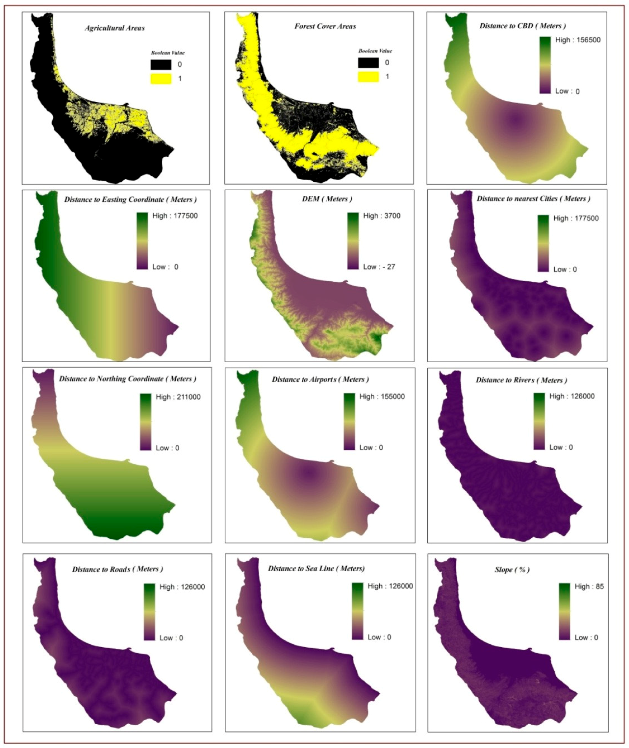
CA, when combined with logistic regression models as done by Wu [
8] and Puertas and Meza [
16], can predict a complex urban reality, thus the potential in being applied in this study. This hybrid framework can form the basic structure of this presented model but when such models are applied in the context of Gilan Province, several considerations will have to be made. The first important consideration is to adopt the CA framework which would suit the realities in the city in a sense that the outputs of the model would provide information at an appropriate scale for urban policy making. The second consideration is to insert the designated variables into the logistic regression models. Given the availability of data, it is important to identify the methods that can be adopted in quantifying the inputs fed into the logistic regression model. The third consideration is to build a link with the policy framework, that is, the CA-based framework and to implement the model by using inputs from the logistic regression model and urban policies in a manner that the model would able to establish forward and backward linkages with urban development and control policies. This consideration should ultimately be reflected in the simulation of urban development and growth. Therefore this study furthers the work conducted on modeling the urban development and growth of Gilan Province Jat et al. [
23], which are mostly examples of modeling urban sprawl but not able to model the development of different land uses. How could some recent applications introduced in the empirical literature on urban growth modeling be adopted in this study?
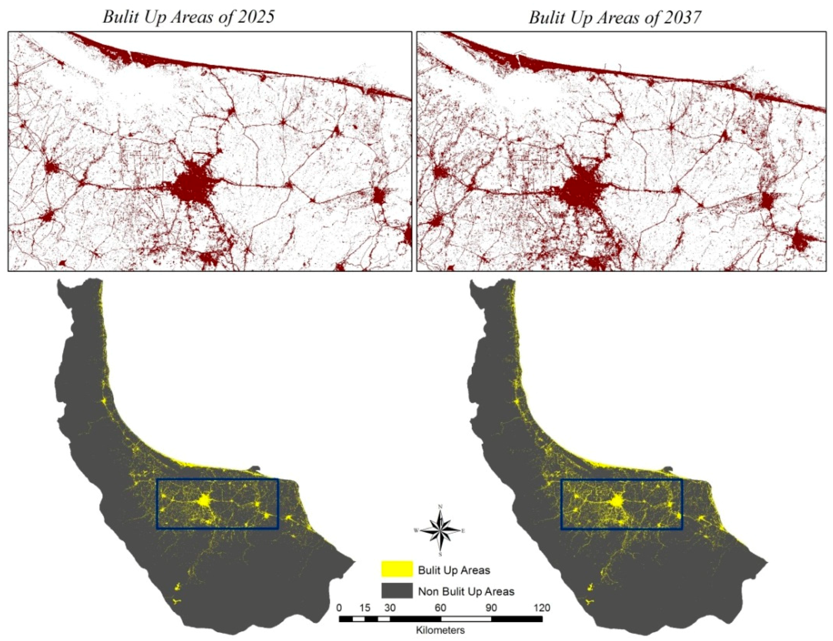
Due to its geo-logistic stance, Gilan experienced significant growth with respect to urban land use areas in recent decades. Annual rural influx expands urban population and promotes the urbanization culture. Unsustainable growth of the city has caused many socioeconomic and environmental problems like reshaping the landscape, emissions, heavy traffic jam, deforestation, and changes in land use. All in all, due to the pleasant climate and picturesque landscape of the Hyrcanian forests and the Caspian Sea have made this part of country one of the most densely populated areas. It is usually the first choice of tourism, domestic and Middle Eastern with low accommodation costs. This fact can pave the way to forecasting sustainable growth in future development by applying the necessary administrative-planned measures and avoiding uncontrolled construction and shapeless growth. Accordingly, this study is run with the objective of presenting a dynamic hybrid model based on LR, MC and CA to forecast the auto-spreading orientation by the years 2025 and 2037 and to answer the question of which land use class would lead to the most negative effects of urban development. The outputs here can equip the decision makers and relevant authorities with future orientations of the restricted urban growth. The main questions for this research are: Which one of the efficiency classes would have the most effect on assessing future plans regarding urban development with respect to its quantitative aspect, orientation and the relevant drivers in a given study zone?; does the combination of Markov and LR in CA method yield an acceptable pattern as an output in urban development for a 12 year period (2025 and 2037) with respect to environmental and socio-economical features of a given zone?


 and
and 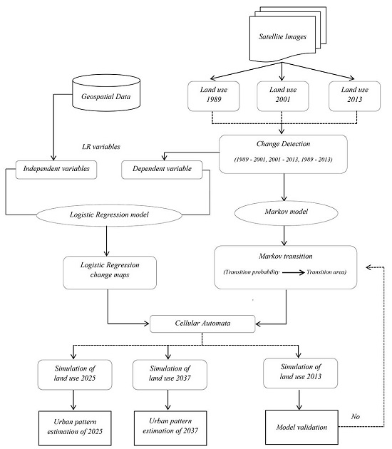


