Simulation and Assessment of Whole Life-Cycle Carbon Emission Flows from Different Residential Structures

Abstract

To explore the differences in carbon emissions over the whole life-cycle of different building structures, the published calculated carbon emissions from residential buildings in China and abroad were normalized. Embodied carbon emission flows, operations stage carbon emission flows, demolition and reclamation stage carbon emission flows and total life-cycle carbon emission flows from concrete, steel, and wood structures were obtained. This study is based on the theory of the social cost of carbon, with an adequately demonstrated social cost of carbon and social discount rate. Taking into consideration both static and dynamic situations and using a social discount rate of 3.5%, the total life-cycle carbon emission flows, absolute carbon emission and building carbon costs were calculated and assessed. The results indicated that concrete structures had the highest embodied carbon emission flows and negative carbon emission flows in the waste and reclamation stage. Wood structures that started the life-cycle with stored carbon had the lowest carbon emission flows in the operations stage and relatively high negative carbon emission flows in the reclamation stage. Wood structures present the smallest carbon footprints for residential buildings.

1. Introduction

Buildings account for 37% of total global energy consumption and carbon emissions, while transportation accounts for 28%, industry accounts for 27%, and the remainder accounts for 8%. Buildings lead the world in energy consumption and carbon emissions [1]. Civilian construction projects can be divided into two main categories: public and residential, with a large proportion of carbon emissions from residential buildings. Moreover, various residential structures have different carbon emission characteristics. In general, concrete, steel, and wood housing units emit different amounts of carbon over their life-cycles. Research using cash flow theory was conducted on the distribution characteristics of carbon emission flows over the whole life-cycle of different residential structures. The differences were compared and analyzed, and the terminal carbon emission flow values were evaluated. This is particularly important in the selection of an optimal low-carbon-emission building structure.

Many scholars have published their calculations of carbon emissions from different residential structures; these include Alcorn and Baird [2], Buchanan and Honey [3], Björklund et al. [4], Canadian Wood Council (CWC) [5], Guggemos et al. [6], Arima [7], Shang et al. [8], Li [9], Rossi et al. [10], Griffin et al. [11], Kim et al. [12], and Li et al. [13]. Their results provide the basic carbon emissions data in the embodied carbon, operations and reclamation stages of various residential structures. Some studies focused on the comparative analysis of concrete and steel structures, concrete structures and wood structures, while some compared all three structures. However, due to differences in the boundaries, methodologies, data sources, and case backgrounds, there were significant differences in the calculated results. To a certain extent, relevant comparisons of the results cannot be made. Thus, an effective normalization method is required to eliminate differences in boundaries, methodologies, regions, etc. to derive the relative ratios of carbon emissions in the life-cycle stages of different residential structures.

Since 2005, extensive research has been performed internationally on the social cost of carbon, coupled tightly with the social discount rate. As an economic indicator for measuring the real impact of carbon emissions on climate change, the social carbon cost reflects the increase in social cost due to carbon emissions–induced climate change in the absence of any reduction measures. Tol [14], Stern [15], Hope [16], Klassen et al. [17], Oliva et al. [18] and the IWGSCC (US Interagency Working Group on the Social Cost of Carbon) [19] all used PAGE2002 (Policy Analysis of the Greenhouse Effect), PAGE2009 or DICE (Dynamic Integrated Climate-Economy) models. The models calculate the social marginal cost under adverse climate conditions and predict the unit social cost of carbon in 2030 or 2050. The research cited above resolved the values of the unit social cost of carbon and social discount rate. However, there are few studies on the impact and degree of impact of the unit social cost of carbon and social discount rate on different industries, especially on construction carbon emissions.

In this paper, residential carbon emissions from the various studies were normalized, abstracting the calculated carbon emissions as flow values to simulate the whole life-cycle carbon emission flow diagrams of concrete, steel, and wood structures. Over the buildings’ whole life-cycles, the total carbon emission flow, absolute carbon emissions, and building cost of carbon were calculated for various structures. This approach removed differences due to factors of data dimension, country, depth of research, case, methodology, and original database to explore the intrinsic characteristics in the whole life-cycle carbon emissions flow from concrete, steel, and wood residential structures.

2. Literature Review

2.1. Whole Life-Cycle Carbon Emissions from Residences

The whole life-cycle of a residence consists of the following stages: materials production and transportation, building construction, operation, maintenance, demolition and reclamation. Normally, carbon dioxide (CO₂) emitted during the materials production and transportation phase and building construction phase are known as embodied carbon. Many research studies have been conducted on embodied carbon in buildings [5,6,7,8,9,10,11,12]. Canadian Wood Council (CWC) [5], Arima [7], Shang et al. [8] and Li [9] performed a comprehensive comparison of embodied carbon in concrete, steel and wood residential structures. Their results are shown in

Table 1. Embodied carbon emissions in different residential structures.

Type	Embodied Carbon (kg CO2/m2)
	CWC	Arima	Shang et al.	Li
Concrete	433	407	338	332
Steel	354	513	278	241
Wood	288	266	172	108

.

The studies found no close relationship between carbon emissions and structure during the operations phase. Guggemos et al. were of the opinion that, in a fifty-year lifetime of a residential building, the differences in carbon emissions of steel and concrete structures are small [6]. Gustavsson et al. found that in the operations phase, energy consumption will not differ because of the structure [20]. Adalberth believed that the differences in carbon emissions from various structures in the operations stage were less than 1% [21]. Cole found that the differences in carbon emissions in the operations stage were negligible [22]. In reality, the carbon emissions in the operations phase of concrete, steel, and wood structures are different, but the disparities are masked by regional economic factors, energy structures and the energy consumption habits of the residents. Thus, it is important to remove these factors to assess the differences in carbon emission flows from different structures.

Glover discovered that the difference between the thermal insulation properties of concrete and wood is small, while the thermal insulation property of steel is worse than that of wood and concrete; the thermal resistance (R-value) of steel is 5% lower than that of wood and concrete [23]. Griffin et al. noted that the specific heats of various construction materials are different: 480 J/kg·K for steel, 840 J/kg·K for concrete, and 1700 J/kg·K for wood [11]. Thus, steel has a low thermal mass and wood has the highest thermal mass. From these values, two basic conclusions followed: (1) the thermal insulation property of steel is worse than that of concrete and wood by at least 5%; and (2) in a comparison of wood and concrete structures, a wood structure has a better thermal insulation property, but the difference in carbon emissions in the operations stage may not be significant.

Gerilla et al. unearthed that for a 150 m² single-family residence, the annual carbon emissions from wood and concrete structures in the operations stage were 1650 kgC and 1900 kgC, respectively, or 40 kg CO₂/m²·year and 47 kg CO₂/m²·year, respectively, upon further conversion [24]. Rossi et al. believed that for a 50-year life-cycle, the carbon emissions from a steel structure in the operations stage were 1050 kg CO₂/m² or 21 kg CO₂/m²·year [10]. Rossi also noted that the carbon emissions from the same construction in the operations stage would be different in different regions: 24.09 kg CO₂/m²·year in Belgium, 38.72 kg CO₂/m²·year in Portugal, and 2.79 kg CO₂/m²·year in Sweden. These differences are closely related to the energy structures of the individual countries. Li et al. found that in the operations stage, carbon emissions in a 50-year life-cycle of a concrete block structure were 1590 kg CO₂/m² or 32 kg CO₂/m²·year [13]. In the absence of data, we assumed that, in the operations stage, the carbon emissions from wood and concrete structures were identical and were 5% higher for a steel structure.

In the demolition and reclamation phase, Pongiglione et al. believed that recycling of steel could result in 30% higher energy savings and lower carbon emissions than a traditional building [25]. Li et al. noted that in the demolition stage, carbon emissions from a concrete block structure were 30.3 kg CO₂/m² and that in the waste materials reclamation stage, carbon emissions were −31.9 kg CO₂/m²; corresponding values for a steel structure were 15 kg CO₂/m² and −319 kg CO₂/m² (assuming a 90% steel recovery rate), respectively [13]. Gustavsson et al. stated that the residual biofuels from wood structures could replace fossil fuels, resulting in higher “negative carbon emissions.” In their study of an 1190 m² apartment building, the negative carbon emissions from biofuel substitution were −105 tC or −324 kg CO₂/m² [20]. Carbon emissions from wood structures in the demolition phase were assumed to be identical to those of steel structures; thus, the carbon emissions from wood structures in the demolition and reclamation stage were −309 kg CO₂/m².

There are significant differences in carbon emissions in the different life-cycle stages of a residence. Emissions from building materials accounted for 9.15%–22.22% of emissions in Taiwan and 15.67%–22.69% in Japan [26]. Lin indicated that over the whole life-cycle of residential buildings, the materials production stage accounted for 22% of carbon emissions, the operations stage accounted for approximately 78%, and the demolition and reclamation stage accounted for 0.44%–0.46% [27]. Ju et al. calculated that the materials and operations phases accounted for 10%–30% and 60%–80% of carbon emissions, respectively, while the demolition and reclamation phase accounted for only 0.18% [28]. She et al. believed that the operation and material production stages had the highest contribution to carbon emissions, accounting for 79% and 19%, respectively, with the demolition stage only accounting for 2% [29]. The results of the various studies were in general agreement: the materials production and construction phase accounted for 15%–20% of carbon emissions, the operations phase accounted for 60%–80%, and the demolition and reclamation phase accounted for 0.5%–2%.

2.2. Social Carbon Cost

Social carbon cost (SCC) refers to marginal losses incurred by an increase in carbon emissions. SCC is the marginal cost due to climate change, i.e., additional costs when no countermeasures to climate change are taken. This cost uses an economic value to reflect the real impact of carbon emissions. The generally negative effects are observed in agriculture, ecology, environment, society, and human health. Current research in social carbon cost is mostly based on marginal cost theory, and its essence is the unit social cost of carbon. Naturally, from the perspective of a cost-benefit framework, SCC can be contrasted to the marginal cost of climate protection. Comparing the marginal social carbon cost to the marginal emission reduction cost, SCC is the marginal benefit due to reduced carbon emissions. The marginal benefit can be derived from the trading prices of carbon on the carbon exchange market. However, SCC is not observable from any market; it is the shadow price of social carbon emissions [14,15,16,17,18,19].

There is a wide range of social carbon costs in various studies. In 2005, Tol arrived at $20/tCO₂ from data in 22 publications [14]. The estimate of Watkiss et al. was $45–$57/tCO₂ [30]. Based on the PAGE2002 model with a very low discount rate of 1.4%, Stern obtained $110/tCO₂ as the marginal cost due to increases in carbon emissions [15]. In 2010, the assessment of the US IWGSCC was $21/tCO₂, and the predicted cost in 2020 was $26/tCO₂ [19]. In 2013, using the PAGE2009 model, Hope calculated the cost to be $106/tCO₂ under the Intergovernmental Panel on Climate Change (IPCC) A1B scenario [16]. In 2014, Oliva et al. conducted technical and economic analyses on rooftop photovoltaic systems in Australia, arriving at a social carbon cost of $20–$30/tCO₂. However, they eventually adopted the value of Hope [18].

The assessment and prediction by the UK Department of Energy & Climate Change indicated the marginal cost of carbon in 2050 to be $165–$495/tCO₂. Applying the PAGE and DICE models, McKinsey & Company calculated the average social carbon cost in 2050 to be $45/tCO₂ and $64/tCO₂, respectively, but the 95% probability value would be $136/tCO₂ [19]. In studying a low-cost pathway for reducing carbon emissions of a particular commercial building and its benefits, Cox et al. believed that the unit social carbon cost would rise from $25/tCO₂ in 2015 to $47/tCO₂ in 2050 (based on the 2009 price) [31].

Although SCC is the shadow price of increasing societal carbon emissions, it cannot be equated to the price of carbon on market exchanges. However, to a certain degree, we can compare it to the trading price of carbon. From 2005 to 2007, in the first phase of the European Union EU-ETS carbon-trading system, the price of carbon increased from €16.85/tCO₂ to €30.45/tCO₂. During the second phase of the EU-ETS, from 2008 to approximately 2012, the price of carbon increased from €15/tCO₂ to €28.59/tCO₂ [32]. The European Union predicted that in the third phase (2013–2020), the price would be maintained at approximately €30/tCO₂ [32,33]. In the US, McKibbin et al. predicted that from 2012 to 2030, the price would increase from $23/tCO₂ to $46/tCO₂ [34]. Sousa et al. assumed that although the price of carbon would fluctuate significantly after 2012, the EU-ETS market would nevertheless stabilize as the market moves toward the intended target [35]. Based on the study conducted on the first and second phases of EU-ETS, Creti et al. believed that the equilibrium price of carbon in 2009–2012 was underestimated [36]. The China Emissions Exchange in Shenzhen successfully commenced operation in June 2013. From 2013 to 2014, the price of carbon on the Shenzhen exchange increased steadily, ranging from 28¥/tCO₂ to 143¥/tCO₂ and stabilizing in the range of 60¥/tCO₂ to 90¥/tCO₂. As of April 2014, the total value traded on the Shenzhen exchange was 191 million ¥ [37].

2.3. Social Discount Rate of Carbon Emissions

The study of SCC is often associated with the social discount rate. Yu compared the present values of expected losses from 1 t of carbon emission in 2005 using 6% and 1% discount rates [38]. Stern, IWGSCC, and Borenstein believed that the social discount rate could be reduced to 2% or 1% [15,19,39]. However, Borenstein recommended a rate of 3% [39]. In 2010, in the assessment of SCC, IWGSCC held that the risk-free rate and climate-risk rate should be included in the social discount rate and that the risk-free rate should be lower than 2.7%. The IWGSCC has usually recommended a discount rate of 3% to the US government for use in policy analyses [19]. Dorbian et al. employed discount rates of 2% and 3% in calculating the social carbon cost from emissions by the aerospace industry [40]. Ackerman et al. Cox et al. and others adopted a discount rate of 3% [19,31]. Klaassen et al. in the technical and economic assessment of a natural gas combined cycle, combined heat and power in the Netherlands and applied a discount rate of 4% [17]. In 2014, Oliva et al. employed a social discount rate of 4%, including 2% risk-free and 2% climate-risk rates [18].

In the studies on the value of the social discount rate cited above, both risk-free and climate-risk rates were taken into consideration. The risk-free rates used were not higher than 2.7% [19] and the climate-risk rate was based on the rate of increase in global carbon emissions. The IPCC noted that from 1750 to 2005, the atmospheric concentrations of CO₂ increased from 280 ppm to 380 ppm at an annualized rate of 1.4% [41]. Fib also noted that over the next 100 years, atmospheric CO₂ concentrations would increase at a 3% annual rate [42]. Stewart et al. predicted that in the 2000–2100 period, it will be possible to divide atmospheric CO₂ concentrations into low, medium, and high levels and three scenarios: IPCC, A1B, and A1F1. A1F1 is considered a very fast economic growth scenario [43]. Based on A1F1, A1B took into consideration the balance between fossil fuel and non-fossil fuel energy sources. The data from Stewart et al. indicated that from 2000 to 2100, the atmospheric CO₂ concentration would be 360–550 ppm under the IPCC scenario, with a 5.3% annual rate of increase; 360–680 ppm under the A1B scenario, with an 8.9% annual rate of increase; and 360–980 ppm under the A1F1 scenario, with a 1.7% rate of increase.

3. Methodology

3.1. Matrix Normalization

Matrix normalization is a form of data standardization. Indicators of different assessments normally have different dimensions and dimensional units that will affect the results of data analysis. To eliminate the dimensional impact of the indicators, the data matrix must be normalized to resolve the issue of comparability among the data indicators. Commonly used normalization methods include sum-product, min–max, and Z-score algorithms [44,45]. The sum-product method normalizes the row and column of the matrix, finds the sum of the rows, and continues on with the normalization of sum-vectors.

Due to the superiority of the sum-product method in the assessment and normalization of multiple data sets, this method was used in this paper to process the various carbon emissions data from the different studies. The carbon emissions matrix was first constructed based on existing data. After normalization, the dimensions of carbon emissions were removed, resulting in the carbon emission flows from different residential structures. Carbon emission flows refer to the value of annual carbon flow over the whole life-cycle of a building, expressed in units of cf.

In the embodied carbon stage, the source of all embodied carbon data come from previous studies. In addition, 433 kg CO₂/m², 354 kg CO₂/m², 288 kg CO₂/m² which are on behalf of concrete structure, steel structure, and wood structure, respectively, come from the study of CWC [5], 407 kg CO₂/m², 513 kg CO₂/m², 266 kg CO₂/m² come from Arima [7], 338 kg CO₂/m², 278 kg CO₂/m², 172 kg CO₂/m² from Shang et al. [8], 332 kg CO₂/m², 241 kg CO₂/m², 108 kg CO₂/m² from the study of Li [9].

The rows of matrix A_em of embodied carbon were first normalized, resulting in Matrix B_em. Matrix A_em and B_em are given by Matrix (1) below:

$$\left(\stackrel{A_{em}}{\begin{array}{c}Concrete\\ Steel\\ Wood\end{array}\begin{array}{cccc}433& 407& 338& 332\\ 354& 513& 278& 241\\ 288& 266& 172& 108\end{array}}\right)\to \left(\stackrel{B_{em}}{\begin{array}{c}\text{Concrete}\\ Steel\\ Wood\end{array}\begin{array}{cccc}0.403& 0.343& 0.429& 0.488\\ 0.329& 0.433& 0.353& 0.354\\ 0.268& 0.224& 0.218& 0.159\end{array}}\right).$$

(1)

Next, the columns of matrix B_em were summed, resulting in vector W_em. Matrix B_em and vector W_em are given by Matrix (2) below:

$$\left(\stackrel{B_{em}}{\begin{array}{c}Concrete\\ Steel\\ Wood\end{array}\begin{array}{cccc}0.403& 0.343& 0.429& 0.488\\ 0.329& 0.433& 0.353& 0.354\\ 0.268& 0.224& 0.218& 0.159\end{array}}\right)\to \left(\stackrel{W_{em}}{\begin{array}{c}Concrete\\ Steel\\ Wood\end{array}\begin{array}{c}1.662\\ 1.469\\ 0.869\end{array}}\right).$$

(2)

Finally, vector W_em was normalized and multiplied by a factor of 1000, resulting in the embodied carbon emission vector F_em for concrete, steel, and wood structures. Vector W_em and vector F_em are given by Matrix (3) below:

$$\left(\stackrel{W_{em}}{\begin{array}{c}Concrete\\ Steel\\ Wood\end{array}\begin{array}{c}1.662\\ 1.469\\ 0.869\end{array}}\right)\to \left(\begin{array}{c}Concrete\\ Steel\\ Wood\end{array}\begin{array}{c}0.416\\ 0.367\\ 0.217\end{array}\right), \mathrm{i}.\mathrm{e}., \left(\stackrel{F_{em}}{\begin{array}{c}{f}_{emc}\\ f_{ems}\\ f_{emw}\end{array}}\right)=\left(\begin{array}{c}416\\ 367\\ 217\end{array}\right)(\mathrm{cf}).$$

(3)

Additionally, at the beginning of the life-cycle, a wood structure has stored carbon. Arima found that the amount of carbon stored in a wood structure exceeded the carbon emitted during construction. In Japan, carbon emissions (total 3,100,000 tC) from buildings less than three stories tall were less than the stored carbon (total 3,400,000 tC) [7]. Based on this information, the ratio of stored and emitted carbon was 34:31 in the embodied carbon phase. Combined with the embodied carbon emission flows of 217 cf for a wood structure, we arrived at −238 cf for the negative carbon emission flows of stored carbon.

Similarly, in calculating the carbon flow in the operations stage, in addition to normalizing the existing results, the ratios for the embodied, operations, and demolition and reclamation phases must be taken into consideration. This paper assumed the ratios to be 19:79:2 [26,29]. The calculation was conducted in two steps: (1) based on the results from various studies on carbon emissions in the operations stage, the carbon flow vector was derived by matrix normalization; and (2) the vector of the initial carbon flow was multiplied by a coefficient, ${\alpha }_{op}=\frac{79}{19\times 50}=0.083$, and then multiplied by an amplification factor of 1000, resulting in the carbon flow vector for the operations phase. Combining the existing calculated values and coefficient α_op, matrix A_op was transformed into the carbon flow vector F_op for the operations stage.

The sources of carbon emission data in the operations stage also come from previous studies. In addition, 40 kg CO₂/m²·year for wood and 47 kg CO₂/m²·year for concrete come from the study of Gerilla et al. [24], 49 kg CO₂/m²·year for steel is calculated by 47 kg CO₂/m²·year with a multiply factor of 1.05, which is based on the assumption that thermal insulation property of steel is worse than that of concrete and wood by at least 5%. Furthermore, 21 kg CO₂/m²·year for steel comes from the study of Rossi et al. [10]. In addition, 20 kg CO₂/m²·year for concrete and wood is calculated by 21 kg CO₂/m²·year divided by 1.05. Here, we also assume that the difference of carbon emissions between wood and concrete structures in the operations stage may not be significant. Data of 32 kg CO₂/m²·year for concrete structures comes from the study of Li et al. [13]. The other two pieces of data—32 kg CO₂/m²·year for wood and 34 kg CO₂/m²·year for steel—are also based on the two assumptions above. Matrix A_op and vector F_op are given by Matrix (4) below:

$$A_{op}=\left(\stackrel{A_{op}}{\begin{array}{c}Concrete\\ Steel\\ Wood\end{array}\begin{array}{ccc}47& 20& 32\\ 49& 21& 34\\ 40& 20& 32\end{array}}\right),F_{op}=\left(\stackrel{F_{op}}{\begin{array}{c}{f}_{opc}\\ f_{ops}\\ f_{opw}\end{array}}\right)=\left(\begin{array}{c}28\\ 29\\ 26\end{array}\right)(\mathrm{cf}).$$

(4)

In the demolition and reclamation stages, −1.6 kg CO₂/m² for concrete structure comes from the study of Li et al. who noted that, in the demolition stage, carbon emissions from a concrete block structure were 30.3 kg CO₂/m² and that, in the waste materials reclamation stage, carbon emissions were −31.9 kg CO₂/m² [13]. Another data −304 kg CO₂/m² for steel structure also comes from the study of Li et al. There are corresponding values 15 kg CO₂/m² for carbon emissions and −319 kg CO₂/m² for reclamation emission [13]. Data of −309 kg CO₂/m² for wood structures comes from the study of Gustavsson et al. [20]. Thus, combined with the ratio coefficient α_re, the matrix A_re can be transformed to the carbon flow vector F_re for the demolition and reclamation phase. Matrix A_re and vector F_re are given by Matrix (5) below:

$$A_{re}=\left(\stackrel{A_{re}}{\begin{array}{c}Concrete\\ Steel\\ Wood\end{array}\begin{array}{c}-1.6\\ -304\\ -309\end{array}}\right),F_{re}=\left(\stackrel{F_{re}}{\begin{array}{c}{f}_{rec}\\ f_{res}\\ f_{rew}\end{array}}\right)=\left(\begin{array}{c}-0.3\\ -52\\ -53\end{array}\right)(\mathrm{cf}),{\alpha }_{re}=\frac{2}{19}=0.105.$$

(5)

3.2. Construction of the Model for Residential Carbon Emission Flows

A cash flow diagram is generally used in assessing different construction schemes for a project. It reflects the states of funds flows over the life-cycle of a construction project and can be used to calculate the net present value, net annual value, and terminal value. These are dynamic economic indicators that can be used to assess the feasibility as well as advantages and disadvantages of different construction schemes. Over the whole life-cycle of a residence, carbon emissions in the construction, operations, and demolition and reclamation stages are analogous to the inflow and outflow of cash, named carbon flows, expressed in units of cf.

In the simulation of carbon emissions flow from different residential structures, the study was divided into three phases based on the whole life-cycle theory of buildings: embodied carbon stage, operations stage, and demolition and reclamation stage. Because the material production, transportation, and construction phases of normal residential buildings are relatively short, the building embodied carbon phase corresponded to time zero in the building’s whole life-cycle in this paper. Although countries, regions and building types are different, the whole life-cycle of all three types of construction is assumed to be 50 years. The operations stage corresponds to year 1 to year 50 in the cycle. The demolition and reclamation phase corresponds to the fiftieth year.

The sum total of carbon flows from all of the phases is the total carbon flow. The total carbon flow can be divided into total static and total dynamic flows, or Cf_k and Cf_dc,k, respectively. Total static carbon flows are the sum total of the carbon flow in each year over the 50-year full life-cycle. Total dynamic carbon flows are the terminal values of carbon flows in each year, taking into account the social discount rate over the entire 50-year life-cycle of a building.

Residential static carbon emissions are given by Equation (1) below:

$$C{f}_k=f_{em,k}+50f_{op,k}+f_{re,k}.$$

(1)

In Equation (1), k denotes the type of building construction, i.e., concrete, steel, or wood; Cf_k denotes the total static carbon flows of type k construction; f_em,k denotes the embodied carbon flows of type k (cf); f_op,k denotes the annual carbon flows of type k in the operations stage; and f_re,k represents the carbon flows of type k in the demolition and reclamation phase (cf).

Taking the social discount rate, i, into account, the dynamic carbon emissions are given by Equation (2) below:

$$C{f}_{dc,k}=f_{em,k}{(1+i)}^{50}+f_{op,k}\times \frac{{(1+i)}^{50}-1}{i}+f_{re,k}.$$

(2)

In Equation (2), Cf_dc,k denotes the dynamic carbon emissions of type k construction; i is the social discount rate; and the rest of the variables are the same as in Equation (1). The unit of Cf_dc,k is also cf. In Equations (1) and (2), the ranges of the values of f_em,k, f_op,k and f_re,k are (0, 1000), (0, 83), and (0, 105), respectively.

The static and dynamic values of carbon flow and total carbon flow are all relative. While beneficial to the selection of residential structure type and assessment of residential functions, the results can be applied to compare different residential structures but cannot be used in the absolute quantitative analysis of carbon emissions of a residence. Absolute carbon emissions refer to the total amount of carbon emitted per area by different residential structures over the whole life-cycle in units of $\mathrm{kg}{\mathrm{CO}}_2/{\mathrm{m}}^2$. This reflects the carbon emissions over the whole life-cycle of a building and is more specific and intuitive than the indicators for the relative assessment of carbon flow. Absolute carbon emissions also include total static and total dynamic amounts, which are called static absolute carbon emissions and dynamic absolute carbon emissions. The whole life-cycle absolute static carbon emissions are given by Equation (3):

$$C{E}_k=C{f}_k\times K_k.$$

(3)

In the above equation, k denotes the residential structure type; Cf_k denotes the total static carbon emission flow of type k; CE_k represents the static absolute carbon emissions of type k; and K_k is the absolute emissions values of carbon emission flow for per cf × m².

The absolute dynamic carbon emissions are given by Equation (4):

$$C{E}_{dc,k}=C{f}_{dc,k}\times K_k.$$

(4)

In the above equation, Cf_dc,k denotes the total dynamic carbon flow of type k; CE_dc,k denotes the dynamic absolute carbon emissions of type k; and K_k is the same as above.

The carbon cost of construction is another indicator corresponding to absolute carbon emissions. The carbon cost of construction is the shadow price of carbon emissions over the whole life-cycle of a building. It represents the whole life-cycle cost due to carbon emissions under the condition that no energy-saving measures are implemented in a construction project. It reflects the opportunity cost of building carbon in the global carbon exchange market, which reflects the benefits of reducing emissions.

The whole life-cycle static carbon costs of construction of various residential structures are given in Equation (5):

$$SC{C}_k=(f_{em,k}{P}_{em}+50f_{op,k}{P}_{op}+f_{re,k}{P}_{re})K_k.$$

(5)

In the above equation, SCC_k denotes the whole life-cycle static carbon cost of construction of type k; P_em, P_op, and P_re represent the unit social carbon cost in the embodied carbon, operations, and demolition and reclamation phases, respectively; and f_em,k, f_op,k, f_re,k, and K_k are the same as in the above equations.

The whole life-cycle dynamic carbon costs of construction of various residential structures are given in Equation (6):

$$SC{C}_{dc,k}=f_{em,k}{(1+i)}^{50}\times K_k\times P_{em}+f_{op,k}\times \frac{{(1+i)}^{50}-1}{i}\times K_k\times P_{op}+f_{re,k}\times K_k\times P_{re},$$

(6)

where SCC_dc,k denotes the whole life-cycle dynamic carbon cost of construction of type k and P_em, P_op, P_re, f_em,k, f_op,k, f_re,k, k, i, and K_k are the same as in the above equations.

4. Results

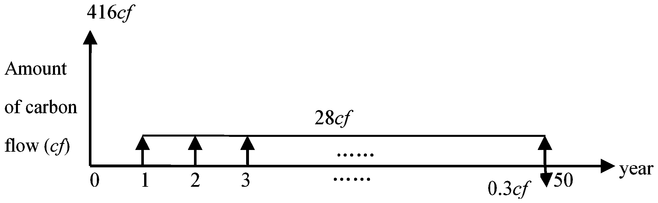
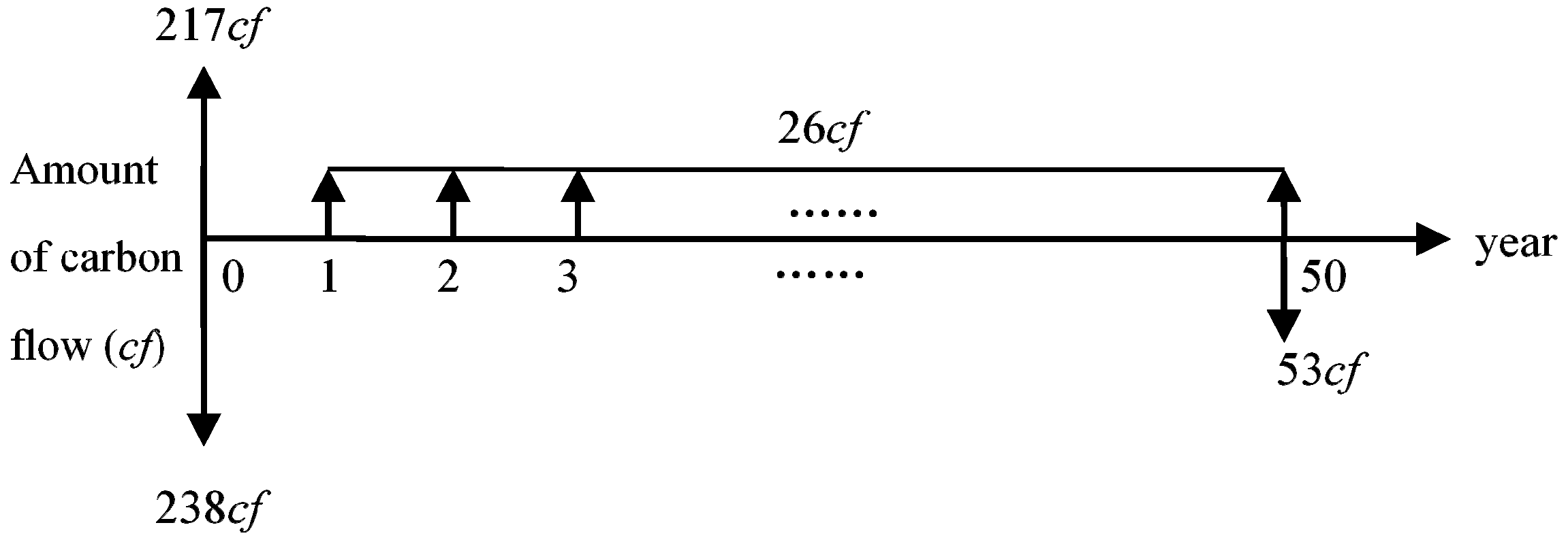
4.1. Simulation of Whole Life-Cycle Carbon Emission Flow Diagrams for Different Residential Structures

In the simulation of residential carbon emission flows, time is the axis, divided into three stages: embodied carbon, operations, and demolition and reclamation. Carbon emissions are shown as positive values, while carbon storage and negative carbon emissions are shown as negative values. A positive carbon emissions flow points up in the diagram, and a negative emissions flow points down. For the three different residential structures, based on normalized carbon flow vectors and values at specific time points (years) in the three life-cycle stages of a building, the carbon emissions flow diagram was simulated as shown in Figure 1, Figure 2 and Figure 3.

There are differences in carbon emissions among the various structures over the whole life-cycle. Concrete had the highest positive embodied carbon emissions flow (416 cf), followed by steel (367 cf) and wood (217 cf). The carbon stored in the wood structure in the embodied carbon stage was −238 cf. In the operations stage, all of the structures had positive carbon flows, and the differences among the three structures were small. All of the structures had negative carbon emissions in the demolition and reclamation stage; the values of steel and wood structures were similar, while the negative carbon value (−0.3 cf) for the concrete structure was negligible. Due to the high recycling rate of steel and the use of wood as a substitute for fossil fuel, both structures had high negative emissions in the demolition and reclamation phase. The difficulty in recycling concrete materials resulted in a low recovery rate. Taking the impact of carbon emissions in demolishing concrete structures into account resulted in a very small negative carbon flow.

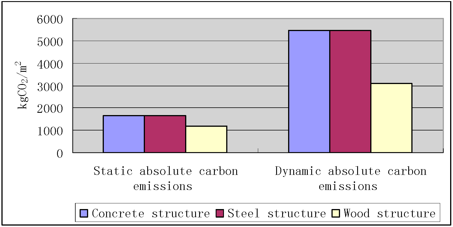
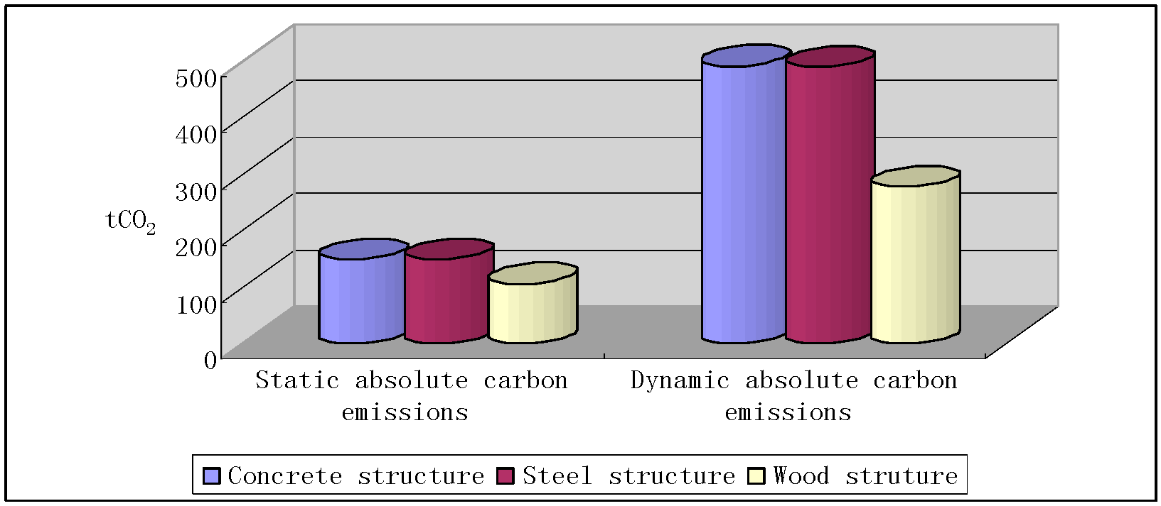
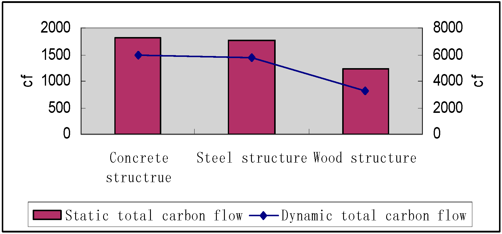
4.2. Assessment of Total Carbon Emission Flows and Absolute Carbon Emissions of Different Residential Structures over Their Whole Life-Cycle

According to the results of CWC [5], Arima [7], Shang et al. [8] and Li [9] pertaining to the emissions of embodied carbon from the three structures (Table 1) and the carbon emissions flow diagrams of embodied carbon for different structures, the indicator K_k for the absolute emissions values for the unit carbon flow of different residential structures can be obtained as follows:

$$K_c=\frac{433+407+338+332}{4\times 416}=0.91(kgC{O}_2/cf·m^2),$$

$$K_s=\frac{354+513+278+241}{4\times 367}=0.94(kgC{O}_2/cf·m^2),$$

$$K_w=\frac{288+266+172+108}{4\times 217}=0.96(kgC{O}_2/cf·m^2).$$

Because the embodied carbon flows of different residential structures were derived from normalized results, despite the significant differences in the four original studies, the indicators of absolute carbon emissions values were in agreement after the average values were divided by the corresponding carbon flows. All three indicators fell in the range of 0.90–1.00.

Furthermore, based on the results of IWGSCC [19], Oliva et al. [18], and Stewart et al. [43] in the calculation and assessment of the dynamic carbon emissions from various residential structures, the risk-free social discount rate was prone to be 2% [18], and the climate-risk rate was 1.5% (A1F1 scenario) [43]. The risk-free rate follows internationally accepted values. The climate-risk rate took into account the results of Stewart et al. [43], i.e., a social discount of 3.5%.

Equations (1) and (3) combined the carbon emission flow diagrams of three residential structures and the three K_k indicators to calculate the static total carbon emission flow and absolute carbon emissions over the whole life-cycle of the various structures. Using a social discount rate of 3.5%, the dynamic total carbon emission flow and dynamic absolute carbon emissions were calculated from Equations (2) and (4). The results are shown in

Table 2. Total carbon flow and absolute carbon emissions over the whole life-cycle of the various residential structures.

Type	Total Carbon Flow (cf)		Absolute Carbon Emissions (kg CO2/m2)
	Static	Dynamic	Static	Dynamic
Concrete	1815.7	5991	1652	5452
Steel	1765	5797	1659	5449
Wood	1226	3236	1177	3107

.

Static total carbon flow and absolute carbon emissions reflect the schematic estimates of carbon emissions over the whole life-cycle of residential structures. Dynamic total carbon flow and absolute carbon emissions are more suitable for assessing a long life-cycle of 50 years because they are based on a dynamic perspective and expound the functional relationship between carbon flow and time. Using time as a basic variable, dynamic total carbon flow and absolute carbon emissions depict the environmental impact of carbon emissions. As global low-carbon politico-economic development changes, the risks of residential carbon emissions evolve with time, becoming more apparent from the initial to later periods of operation. Therefore, the terminal values of dynamic total carbon flow and absolute carbon emissions are more objective than static indicators for the whole life-cycle of a residential structure. Dynamic indicators should be regarded as primary indicators, with static indicators as secondary when estimating carbon emissions over the whole life-cycle of various residential structures.

Figure 4 depicts the difference between the dynamic and static total carbon flows of various structures over the whole life-cycle of residential structures. The differences between concrete and steel structures are small, while the total carbon flows from wood structures are lower. Dynamic and static total carbon flows have similar characteristics; i.e., concrete is the highest and wood the lowest. The line graph for the dynamic case shows a more prominent drop for the wood structure. Figure 5 reflects the differences in static and dynamic absolute carbon emissions among the three structures. In the static case, the variation in the curve is small, and the difference among the structures is small: wood is 0.71 of concrete and steel. In the dynamic case, there is a significant rise in the curve for steel and concrete, and the differences among the three structures are obvious. Thus, from the long 50-year life-cycle perspective, there are significant differences in the absolute carbon emissions among the three structures, with wood having the lowest value at 0.57 of concrete and steel.

Using an area of 90 m² for a typical residential unit, the whole life-cycle static and dynamic absolute carbon emissions for a concrete structure are 149 tCO₂ and 491 tCO₂, respectively; the corresponding numbers for a steel unit are similar as 149 tCO₂ and 490 tCO₂, respectively, while those for a wood structure are 106 tCO₂ and 280 tCO₂, respectively, as shown in Figure 6.

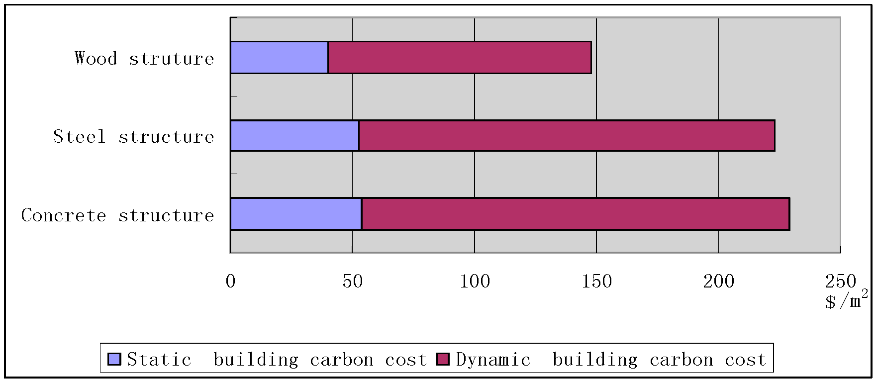
4.3. Assessment of Whole Life-Cycle Building Carbon Cost of Various Structures

The unit social carbon cost based on previous studies formed the basis of this research; in this study, the cost was assumed to be $25/tCO₂ [14,18,19], which reflects the current cost. The average annual cost over the next 50 years was assumed to be $35/tCO₂ [32,33], and in the fiftieth year, the average annual cost was assumed to be $58/tCO₂ [18,19,31]. The unit social carbon cost in the embodied carbon, operations, and demolition and reclamation stages corresponds to the current unit cost of carbon, the average annual social carbon cost over the next 50 years, and the cost in the fiftieth year, respectively. The unit carbon costs in the different phases are shown in

Table 3. Unit social carbon cost of residences in the various phases.

Social Carbon Cost ($/kg CO2)
Embodied Carbon Phase	Operations Phase	Demolition and Reclamation Phase
0.025	0.035	0.058

.

With a social discount rate of 3.5%, Equations (5) and (6) were used to calculate the carbon cost of construction in the life-cycle stages, as shown in

Table 4. Building carbon costs of various structures in the life-cycle stages.

Building Carbon Cost ($/m2)
Type	Static Building Carbon Cost	Dynamic Building Carbon Cost
Concrete	54	175
Steel	53	170
Wood	40	109

.

The ratios of static building carbon costs of concrete, steel and wood structures over the life-cycle are 54:53:40, or 1.35:1.33:1. The corresponding dynamic ratios are 175:170:109, or 1.61:1.56:1. Figure 7 depicts the difference in static and dynamic building carbon costs over the life-cycle.

The wood structure has the lowest building carbon cost, while concrete has the highest. This indicates that in future international carbon trade and political maneuvers, wood structures have the lowest societal carbon cost risk, while concrete has the highest. Using dynamic building carbon cost as an example, the risk of a wood structure is 38% lower than that of concrete and 36% lower than that of steel. Thus, building carbon cost should be an important factor in addition to actual construction cost.

5. Discussion

An increase in existing publications and data led to higher accuracy in the calculation and simulation of whole life-cycle residential carbon emission flows based on matrix normalization. At the present time, data for carbon emissions in building operations and demolition and reclamation phases are relatively lacking. Orders n (3 × n) of the embodied carbon emissions matrix (A_em), operations matrix (A_op), and demolition and reclamation matrix (A_re) can be infinitely expanded from the foundation provided by existing studies. The research can also be extended to different functional buildings (m × n) to construct the matrices (A_em, A_op, and A_re) of different functions for the simulation of carbon emission flow.

In the matrix normalization process, the difference in perspective and understanding of the ratio of carbon emissions in the different phases of a building’s full life-cycle will affect the coefficients α_op and α_re. This will change the value and range of carbon flows in the operations and demolition and reclamation stages. Differences in the understanding of the thermal insulation properties of the various structures will change the carbon flow values in the operations phase, for example, whether the thermal insulation properties of a steel structure are lower than wood and concrete structures by 5% or more or whether the thermal insulation properties of concrete and wood structures are the same. Differences in the understanding of the recovery rate will change the carbon flow value in the demolition and reclamation phase; e.g., whether the recovery rate of steel is 90% or changes in the calculation of the negative carbon emission of wood recovery will change the carbon flow value. However, these changes will not fundamentally alter the relative characteristics of the three structures and their environmental impacts.

If the social discount rate drops to 2%, the dynamic total carbon flow and absolute carbon emissions will decrease by 35%–42%. In this case, the magnitude of the decrease is essentially the same as that of the social discount rate. If the social discount rate rises to 5%, the dynamic total carbon flow and absolute carbon emissions will increase by 59%–78%, higher than the rise in the social discount rate. However, the change in value will not fundamentally alter the structures’ relative carbon emission impact. As the social discount rate drops, the advantage of wood relative to concrete and steel structures will be less significant. For example, with a social discount rate of 2%, the total carbon flow and absolute carbon emissions of wood structures are 0.60 and 0.62 of concrete and steel structures, respectively. Conversely, wood structures have a clear advantage over concrete and steel structures when the social discount rate rises. At a 5% social discount rate, the total carbon flow and absolute carbon emissions of wood structures are 0.48 and 0.50 of concrete and steel structures, respectively.

6. Conclusions

This paper is based on existing calculations of residential carbon emissions. By normalizing the carbon emission matrices and adjusting the coefficients, various factors leading to differences in the previous studies were eliminated. This normalization allowed for exploration of the intrinsic characteristics of carbon emission flows over the whole life-cycle of concrete, steel, and wood structures.

For carbon emission flows from three residential structures, our findings are as follows:

1)

In the embodied carbon stage, concrete structures have the highest carbon flow, followed by steel, while wood structures have net negative carbon flow.

2)

In the operations stage, there are no significant differences in carbon emission flows among the structures.

3)

In the demolition and reclamation stage, due to the recyclability of steel and use of wood as a substitute fuel source, both structures have large negative carbon emissions, whereas due to difficulties in materials recovery and thus a low recovery rate, concrete structures have negligible negative carbon emissions.

For the assessment of residential carbon emission flows over the whole life-cycle:

1)

Concrete structures have the highest total carbon flow, absolute carbon emissions, and dynamic building carbon cost. Concrete has a higher risk in low-carbon residential construction.

2)

Wood structures have the lowest values in all indicators. Wood structures are the best option for low-carbon residential construction.

References

1. Brinnel, V.; munstermann, S.; Bleck, W.; Foldmenn, M.; Reese, S. Structural requirements and material solutions for sustainable buildings. Rev. Metall. 2013, 110, 37–46. [Google Scholar] [CrossRef]
2. Alcorn, J.A.; Baird, G. Use of a hybrid energy analysis method for evaluating the embodied energy of building materials. Renew. Energy 1996, 8, 319–322. [Google Scholar] [CrossRef]
3. Buchanan, A.H.; Honey, B.G. Energy and carbon dioxide implications of building construction. Energy Build. 1994, 20, 205–217. [Google Scholar] [CrossRef]
4. Björklund, T.; Jönsson, Å.; Tillman, A.M. LCA of building frame structures: Environmental impact over the life cycle of concrete and steel frames. Int. J. Life Cycle Assess. 1998, 3, 216–224. [Google Scholar]
5. Canadian Wood Council (CWC). IBS4—Sustainability and Life Cycle Analysis for Residential Buildings [EB/OL]. Available online: http://cwc.ca/publications/technical/fact-sheets/ (accessed on 6 August 2016).
6. Guggemos, A.A.; Horvath, A. Comparison of environmental effects of steel- and concrete-framed buildings. J. Infrastruct. Syst. 2005, 11, 93–101. [Google Scholar] [CrossRef]
7. Arima, T. Wood construction as “Urban Forest Reserves”. In Proceedings of the 11th World Conference on Timber Engineering, Trentino, Italy, 20–24 June 2010.
8. Shang, C.J.; Chu, C.L.; Zhang, Z.H. Comparison of different structures carbon emissions in building lifecycle. Build. Sci. 2011, 27, 66–70. [Google Scholar]
9. Li, S.H. Embodied Environmental burdens of wood structure in Taiwan compared with reinforced concrete and steel structures with various recovery rates. Appl. Mech. Mater. 2012, 174, 202–210. [Google Scholar] [CrossRef]
10. Rossi, B.; Marique, A.F.; Reiter, S. Life-cycle assessment of residential building in three different European locations, case study. Build. Environ. 2012, 51, 402–407. [Google Scholar] [CrossRef]
11. Griffin, C.T.; Donville, E.; Thompson, B.; Hoffman, M. A multi-performance comparison of long-span structural systems. In Proceedings of the 2nd International Conference on Structures and Architecture, Guimaraes, Portugal, 24–26 July 2013.
12. Kim, S.; Moon, J.H.; Shin, Y.; Kim, G.H.; Seo, D.S. Life comparative analysis of energy consumption and CO2 emissions of different building structural frame types. Sci. World J. 2013, 2013, 175702. [Google Scholar] [CrossRef] [PubMed]
13. Li, F.; Cui, S.H.; Gao, L.J. Comparative study on the carbon footprint of brick and concrete shear wall building structures. Environ. Sci. Technol. 2012, 35, 18–22. [Google Scholar]
14. Tol, R.S.J. The marginal costs of carbon dioxide emissions: An assessment of the uncertainties. Energy Policy 2005, 33, 2064–2074. [Google Scholar] [CrossRef]
15. Stern, N. The stern review on the economic effects of climate change. Popul. Dev. Rev. 2006, 32, 793–798. [Google Scholar]
16. Hope, C. Critical issues for the calculation of the social cost of CO2: Why the estimates from PAGE09 are higher than those from PAGE2002. Clim. Chang. 2013, 117, 531–543. [Google Scholar] [CrossRef]
17. Klaassen, R.E.; Patel, M.K. District heating in the Netherlands today: A techno-economic assessment for NGCC-CHP (Natural Gas Combined Cycle combined heat and power). Energy 2013, 54, 63–73. [Google Scholar] [CrossRef]
18. Oliva, H.S.; MacGill, I.; Passey, R. Estimating the net societal value of distributed household PV systems. Sol. Energy 2014, 100, 9–22. [Google Scholar] [CrossRef]
19. Ackerman, F.; Stanton, E.A. Climate Risks and Carbon Prices: Revising the Social Cost of Carbon. Economics 2012, 6, 1–27. [Google Scholar] [CrossRef] [Green Version]
20. Gustavsson, L.; Sathre, R. Variability in energy and carbon dioxide balances of wood and concrete building materials. Build. Environ. 2006, 41, 940–951. [Google Scholar] [CrossRef]
21. Adalberth, K. Energy Use and Environmental Impact of New Residential Buildings; Lund University: Lund, Sweden, 2000. [Google Scholar]
22. Cole, R.J. Energy and greenhouse gas emissions associated with the construction of alternative structural systems. Build. Environ. 1998, 34, 335–348. [Google Scholar] [CrossRef]
23. Glover, J.; White, D.O.; Langrish, T.A.G. Wood versus concrete and steel in house construction—A life cycle assessment. J. For. 2002, 100, 34–41. [Google Scholar]
24. Gerilla, G.P.; Teknomo, K.; Hokao, K. An environmental assessment of wood and steel reinforced concrete housing construction. Build. Environ. 2007, 42, 2778–2784. [Google Scholar] [CrossRef]
25. Pongiglione, M.; Calderini, C. Material savings through structural steel reuse: A case study in Genoa. Resour. Conserv. Recycl. 2014, 86, 87–92. [Google Scholar] [CrossRef]
26. Luo, Z.X. Study on the computation method of CO2 emission from building materials and the strategies for emission reduction. Constr. Sci. 2011, 27, 1–7. [Google Scholar]
27. Lin, B.R.; Liu, N.X.; Peng, B.; Zhu, Y.X. Comparative study on international building life-cycle energy consumption and CO2 emission. Constr. Sci. 2013, 29, 22–27. [Google Scholar]
28. Ju, Y.; Chen, Y. Study on the computation method of building carbon emission under the whole life-cycle theory—Statistical analyses based on 1997–2013 publications on CNKI. Resid. Technol. 2014, 5, 32–37. [Google Scholar]
29. She, J.Q.; Zhang, Y.B.; Qi, S.J. Whole life-cycle carbon emission characteristics and emission reduction strategy of public building in subtropical region—Case study on Xiamen. Constr. Sci. 2014, 2, 13–18. [Google Scholar]
30. Watkiss, P.; Downing, T.; Handley, C.; Butterfield, R. The Impacts and Costs of Climate Change, AEA Technology Environment, Stockholm Environment Institute; Commissioned by European Commission DG Environment: Oxford, UK, 2005. [Google Scholar]
31. Cox, M.; Brown, M.A.; Sun, X. Energy benchmarking of commercial buildings: A low-cost pathway toward urban sustainability. Environ. Res. Lett. 2013, 8, 035018. [Google Scholar] [CrossRef]
32. Mizrach, B. Integration of the global carbon markets. Energy Econ. 2012, 34, 335–349. [Google Scholar] [CrossRef]
33. Boersen, A.; Scholtens, B. The relationship between European electricity markets and emission allowance futures prices in phase II of the EU (European Union) emission trading scheme. Energy 2014, 74, 585–594. [Google Scholar] [CrossRef]
34. McKibbin, W.J.; Morris, A.C.; Wilcoxen, P.J. Pricing carbon in the U.S.: A model-based analysis of power-sector-only approaches. Resour. Energy Econ. 2014, 36, 130–150. [Google Scholar]
35. Sousa, R.; Aguiar-Conraria, L.; Soares, M.J. Carbon financial markets: A time-frequency analysis of CO2 prices. Available online: http://repositorium.sdum.uminho.pt/handle/1822/27957 (accessed on 6 August 2016).
36. Creti, A.; Jouvet, P.A.; Mignon, V. Carbon price drivers: Phase I versus Phase II equilibrium. Energy Econ. 2012, 34, 327–334. [Google Scholar] [CrossRef]
37. Chen, X.H. Selling 27K Tons of “Carbon” in 11 Months. Shenzhen Economic Daily, 11 June 2014; A04. [Google Scholar]
38. Yu, M.K.W. The social discount rate on climate change: A case study of Part L of Schedule 1 of the UK Building Regulations—Conservation of fuel and power. Prop. Manag. 2006, 24, 144–161. [Google Scholar]
39. Borenstein, S. The private and public economics of renewable electricity generation. J. Econ. Perspect. 2012, 26, 67–92. [Google Scholar] [CrossRef]
40. Dorbian, C.S.; Wolfe, P.J.; Waitz, I.A. Estimating the climate and air quality benefits of aviation fuel and emissions reductions. Atmos. Environ. 2011, 45, 2750–2759. [Google Scholar] [CrossRef]
41. IPCC. Fourth Assessment Report of the Intergovernmental Panel in Climate Change; Cambridge University Press: Cambridge, UK, 2007. [Google Scholar]
42. Fib. Model Code for Service Life Design; Bulletin 34; Fib: Lausanne, Switzerland, 2006. [Google Scholar]
43. Stewart, M.G.; Wang, X.; Nguyen, M.N. Climate change impact and risks of concrete infrastructure deterioration. Eng. Struct. 2011, 33, 1326–1337. [Google Scholar] [CrossRef]
44. Wei, C.P. The optimization basis and properties of the sum-product method in AHP. Syst. Eng. Theory Pract. 1999, 9, 113–115. [Google Scholar]
45. He, B.; Chen, C. Theoretical derivation of ranking results in analytic hierarchy process. J. Yunnan Norm. Univ. 2002, 4, 11–14. [Google Scholar]
Figure 1. Carbon emissions flow diagram of a concrete structure.
Sustainability 08 00807 g001
Figure 2. Carbon emissions flow diagram of a steel structure.
Sustainability 08 00807 g002
Figure 3. Carbon emissions flow diagram of a wood structure.
Sustainability 08 00807 g003
Figure 4. Whole life-cycle total carbon emission flow.
Sustainability 08 00807 g004
Figure 5. Whole life-cycle absolute carbon emissions.
Sustainability 08 00807 g005
Figure 6. Whole life-cycle absolute carbon emissions from a 90 m2 residence.
Sustainability 08 00807 g006
Figure 7. Static and dynamic building carbon costs of various residential structures.
Sustainability 08 00807 g007