Article

Assessment of Environmental and Economic Impacts of Vine-Growing Combining Life Cycle Assessment, Life Cycle Costing and Multicriterial Analysis

Department of Agriculture (AGRARIA), Mediterranean University of Reggio Calabria, Feo di Vito, Reggio Calabria 89122, Italy
*
Author to whom correspondence should be addressed.
Sustainability 2016, 8(8), 793; https://doi.org/10.3390/su8080793
Submission received: 15 April 2016 / Revised: 8 July 2016 / Accepted: 5 August 2016 / Published: 13 August 2016

Abstract

:
The wine sector is going through a significant evolution dealing with the challenges of competition issues in international markets and with necessary commitments to sustainability improvement. In the wine supply chain, the agricultural phase represents a potential source of pollution and costs. From the farmers’ point of view, these contexts require them to be more attentive and find a compromise among environmental benefits, economic benefits, and costs linked to farming practices. This paper aims to make a sustainability assessment of different wine-growing scenarios located in Calabria (Southern Italy) that combines conflicting insights, i.e., environmental and economic ones, by applying Life Cycle Assessment (LCA) and Life Cycle Costing (LCC) to identify the main hotspots and select the alternative scenarios closest to the ideal solution through the VIKOR multicriteria method. In particular, the latter allowed us to obtain synthetic indices for a two-dimensional sustainability assessment. Conventional practices associated to the espalier training system represent the best compromise from both environmental and economic points of view, due to the higher yield per hectare. The choices regarding Functional Unit (FU) and indicators were shown to have a high influence on results.

1. Introduction

According to the definition provided in 1989 by the American Agronomy Society, sustainable agriculture can be considered as an activity “that, over the long term, enhances environmental quality and the resource base on which agriculture depends; provides for basic human food and fiber needs; is economically viable; and enhances the quality of life for farmers and society as a whole” [1]. Since then, a heightened scientific debate occurred over which paradigms, approaches and methodologies are more appropriate to solve these issues, and how to consider the multifarious aspects and implications characterizing a complex agricultural [2]. In this sense, Kajikawa et al. [3] affirmed that, within the latest scientific literature on sustainability discourses, agricultural sustainability is the more representative disciplines-focus issue, proving the relevance of research advances in this field.
Nevertheless, the growing need to find new methods and tools for the impacts assessment of agricultural sector is confirmed by its crucial responsibility in generating negative externalities, mainly due to production practices. For example, it is well known that the reduction of pollution impacts represents the most ambitious challenge for developed countries. This aim has been strongly supported by the European Union that, in coherence with the “Europe 2020” strategy, works toward the goal of 20% emissions reduction, 20% increase of renewable energy and 20% increase in energy efficiency [4]. The agro-food sector is one of the most polluting economic sectors [5], producing around 10% of European emissions of greenhouse gases [6], around 90% of acidifying pollutants emissions and depleting nearly 34% of freshwater resources [7]. These phenomena are attributable to the large use of fertilizers, methane emissions by ruminant’s digestion, the use of agricultural machines etc.; furthermore, the rate of growth of these environmental externalities is faster than the regeneration rate of ecosystems. The resulting damages such as global warming, loss of biodiversity, energy resources depletion and wastes production, in the long term, could lead to serious social and economic consequences.
At the same time, the conscious adoption of more environmental sustainable practices, necessarily, has to meet the economic needs of entrepreneurs, in terms of farmers’ income stabilization, costs reduction, productivity and competitiveness increase through marketing strategies based on value-added products supply. The recognition of the multi-dimensional requirements for a sustainable agricultural production entails a special effort to provide solutions applicable by real subjects to real problems, overcoming the traditional single-criterion decision-making [8].
As is the case with the most important agro-food supply chains, the wine sector is going through a significant evolution dealing with the challenges of the competition on international markets, and answering to commitments to sustainability improvements. Mariani and Vastola [9] argued that the main perspectives in sustainable winegrowing are related mainly to producers and consumers’ needs. In particular, from the farmers’ point of view, the urgency is to balance environmental protection, economic benefits, and costs linked to sustainable practices. Concerning the consumers, the objective can be reached through marketing strategies oriented at fostering the confidence toward sustainable wine, for example by improving communication through labels. Indeed, findings of several consumer’s analyses suggest that wine firms should pay attention to the requirements of environmentally conscious consumers [10], and sustainable certification on wine labels may help wineries to become more competitive by differentiating their products.
OIV [11], in its guidelines, defined sustainable vitiviniculture as a global strategy that takes into account, both in the agricultural and processing phases, the economic sustainability of a territory producing quality products as well as environmental risks, product safety and consumers’ health, as well as many other social aspects (e.g., cultural heritage, history).
In this context, the Life Cycle Thinking (LCT) conceptual model was conceived as a new approach to investigate all impacts (i.e., environmental, economic and social ones) generated by products and services life cycles, from planning to disposal [12]. Under this conceptual model, many methodologies were developed, included in the so-called Life Cycle Management (LCM) framework, useful for the evaluation of all production phases, “from cradle to grave”, in order to make products and services more environmental, economic and societal friendly. This methodological toolbox has gained great consensus as support for strategies to decrease footprints, to add value to products and supply chains and to improve the sustainability performances of a business or organization [13]. In particular, to evaluate the environmental and economic impacts, respectively, Life Cycle Assessment (LCA) and Life Cycle Costing (LCC) were developed and, successively, validated through standardization processes [14,15,16].
What emerges in most of the studies available in literature, is the impelling necessity to combine, integrate, and/or find a compromise between conflicting purposes and criteria of sustainability, especially when different typologies of stakeholders are implicated. To conduct a sustainability assessment by combining different dimensions, Multi-Criteria Decision Analysis (MCDA) tools can be useful to compare results of different analyses and to balance, for example, environmental, social and economic data [17,18,19]. In particular, there is a growing scientific literature on the advantages of combining MCDA with life cycle tools.
The purpose of the present study is to make a sustainability assessment that combine conflicting insights (environmental and economic ones), applying LCA and LCC methodologies to identify main hotspots and selecting the alternative scenarios closest to the ideal solution through the VIKOR method [20,21,22]. The reason for the choice of this method, among other MCDA tools, is threefold: it entails a higher sensitivity analysis compared to other MCDA methods; its software package is flexible [23]; it allows to solve discrete decision problems by determining the compromise solution with incommensurable or discordant criteria [24].
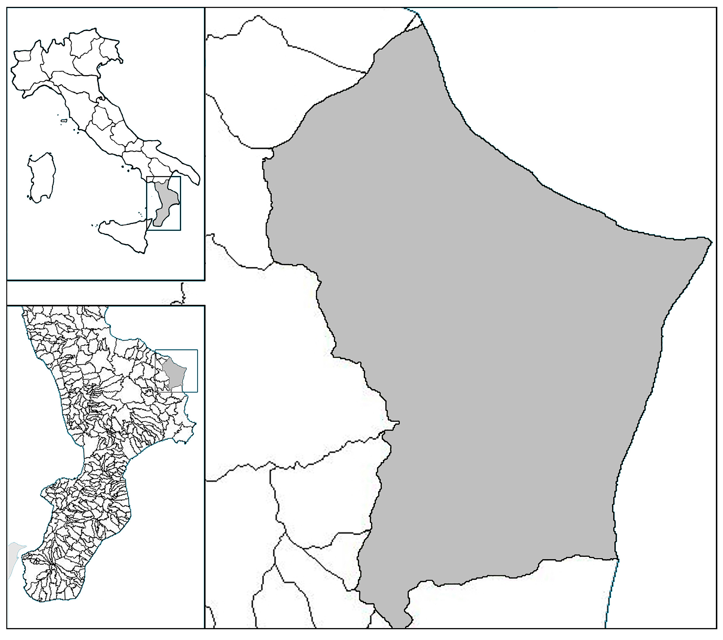
The methodological proposal is then applied to a real case study, i.e., the sustainability assessment of grapevine production systems in Cirò production area, in Calabria (South Italy), with the purpose to find a compromise between the economic concerns of farmers, and the environmental issues to satisfy the claims of more conscious consumers. The methodology allowed us to obtain indices of sustainability to implement a two-dimensional sustainability assessment, merging the values of different criteria in a single indicator.
Furthermore, the study also contributes to expanding the knowledge of grape vine production linked to environmental and economic concerns, through the extension of system boundary to the whole life cycle of vineyard and providing a location-specific dataset useful as reference for LCA practitioners.
Findings can be useful to interpret economic and environmental sustainability issues and to accompany decision-making processes providing transparent, perceivable and systematic information about trade-offs involved in a complex production process.

2. Methodological Background

LCA methodology has raised a growing interest, leading to the development of many applications within different productive systems, including the food farming sector. The latter represents a challenging field due to the need to solve complex matters from both methodological and technical point of views [25]. Regarding the application of LCA to agro-food productions, several studies are available in the literature [26,27,28]; in particular, research in fruit sector has assumed a growing relevance starting from 2005. Concerning the wine sector, in the last decade there was an increasing interest in LCA applications, underlining the great relevance that the environmental issues play also in this sector [29,30].
Splitting the life cycle of wine into five sub-systems (farming, transformation, packaging, distribution and use), it has been found that the agricultural phase represents the most important potential source of greenhouse gas emissions, due to the consumption of fossil fuels for mechanical operations [30,31,32]. Comparative assessment is one of principal types of application performed by international scholars. Regarding the farming phase, several studies have aimed to compare different agricultural management, focusing in particular on comparison between conventional and organic or biodynamic cultivation [33,34,35,36,37].
The most common Functional Unit (FU) applied in LCA studies on wine growing is the mass unit as the bottle, the volume of wine or the mass of grapes [31,38,39]. Only few studies used a cultivated area unit to compare different farming strategies [35,40]. Among the studies that declare a system boundary from “cradle to grave”, the agricultural phase considered only consists in the full production phase, disregarding other phases such as the planting or the growing and decreasing production phases [41,42,43,44]. Only a few papers include the planting of a vineyard (e.g., [45,46]) and a minority considers the whole cultivation cycle (e.g., [40]). According to Petti et al. [29], as in the case of every perennial crop, it is important to assess the overall life cycle of a vineyard, including planting, the unproductive phase, as well as the productive senescence phases and removal. Most studies restrict the system boundaries by excluding the consumption phase because of a lack of significant data; in doing so, the impact generated is limited to transportation from the point of sale to the place of consumption—and for some types of product to refrigeration facilities—and can be omitted because it is negligible [42,43].
Some specific issues are often neglected because of the lack of data or the difficulty to apply specific estimation models (e.g., wastewater treatments or emissions of herbicides and pesticides) [29]. One of the most significant issues related to LCA methodology concerns data quality. The agricultural production systems are strictly linked to the natural environment; for this reason, the use of plurennial average data avoids misinterpretations due to particular natural phenomena [47]. On the other hand, the use of average data may increase data uncertainty, making difficult the understanding of individual scenario results [48]. Most of studies use direct data collection from primary sources for grape growing, winemaking and bottling, while data for fuel and electricity supply chain, manufacturing and transport of agrichemicals, wine additives and glass bottles are often derived from secondary sources [29].
Generally, most of the LCA studies concerning wine production are based on the evaluation of more impact categories, even if many times the assessment is also made by calculating a single environmental issue [36,49,50,51,52,53,54,55].
Literature analysis showed that LCA represents an appropriate methodology to assess grape-growing management systems, because it allows pointing out every environmental hotspot linked to the life cycle and to design more sustainable process according to its results. However, there are some issues that can limit the use of this methodology, as the high engagement of resources (in terms of human resources, costs and time), especially in data gathering, but also the difficulty for practitioners to conduct a complete and comprehensive study and the complexity of results to be interpreted.
From an economic point of view, LCC represents the most common economic tool used jointly with LCA [56,57]. LCC allows us to assess all costs incurred throughout the whole production process, from acquisition phase to final disposal of a product or system [58,59]. The principal application of LCC insights is to identify the main cost factors on which the firm’s management should be focused to reduce them and optimize the economic performances of enterprises [60]. Although LCC was originally developed in the management accounting context, as an analysis tool for ranking different investment alternatives, in the last years different procedures and several standards were developed for performing and harmonizing the method [16,61].
Many of these approaches are based on cash flows models, in which future costs are actualized to their present value. In this sense, the economic evaluation is usually done from a solely financial point of view. This typology of LCC has been identified as Conventional LCC [62,63], which follows the guidelines by [16]. However, a univocal procedure to calculate costs does not yet exist [63] and, therefore, inconsistent approaches and conceptual confusions may lead to misinterpretation [64].
Since LCC is not standardized like LCA [65], several efforts have been undertaken for integrating life cost analysis and LCA [61,66,67,68,69]. However, issues have been found in the substantial difference inherent the computational structures of the two methods. These differences mainly concern purposes, system boundaries, flows accounting and time treatment. While LCA considers all processes connected to the physical life cycle of the product including background processes [70] from a multi-stakeholder perspective, conventional LCC takes into account all activities causing cost and benefit monetary flows during the product’s lifetime from a single-stakeholder perspective. Heijungs et al. [71] have attempted adapting the computational structures of LCC and LCA by means of a matrix-based approach that can be applied to both physical and monetary flows. Recently, Moreau and Weidema [72] challenged the validity of this study, by highlighting some conceptual errors inherent in the methodological approach.
Concerning the LCA-LCC combined applications to food products, although LCC is a discounted cash flows analysis applied to durable goods, Roy et al. [73] showed that LCC can be used as a decision support tool within LCA of food products. However, the scientific literature provides few applications of LCC to food products and, more generally, to non-durable products, and the adopted approaches vary significantly [65]. Focusing on agricultural production, in some studies, LCC was integrated with LCA analysis through the adoption of a common database, considering the same functional unit and system boundary and assessing in monetary terms the physical flows resulting from the life cycle inventory. The resultant costs from all unitary processes have been aggregated for all life-cycle phases during the whole lifetime. Notarnicola et al. [74] adopted this approach to assess the environmental and cost profiles of conventional and organic extra-virgin olive oil production, by combining LCA and LCC methods, and compared their environmental performances and highlighted the reasons for the higher market price of the organic oil.
In some other studies, the LCC approach was combined with a cash flow analysis in order to determine the profitability of agricultural systems through specific economic indicators. This is the case of De Gennaro et al. [75], who examined the environmental and economic performances of two innovative olive-growing systems by using a model of LCC based on input-output analysis, and in particular, whether high trees density orchards were able to reduce production costs without worsening environmental sustainability. Mohamad et al. [76] investigated the environmental impacts and economic performances of two organic and conventional olive production systems, focusing on field agricultural practices, with the aim to recognize the hotspots of each system and optimizing olive field operation. De Luca et al. [77] analyzed the level of sustainability of different Clementine production systems—conventional, integrated and organic—from both an economic and environmental standpoint: results allowed to compare and to rank performances of each scenario for every methodology applied. Pergola et al. [78] added, to the combination of LCA and LCC methods, an energy analysis to compare organic and conventional farming systems of lemon and orange productions, in order to evaluate also their energy consumption. To the authors’ knowledge, apart from Amienyo [79], who performed a comparative analysis in the beverage sector by coupling LCA, LCC and social indicators, there are only two works that evaluate the economic performance of grapevine production systems applying LCC and/or LCA (e.g., [40,80]).
Concerning, in a broad sense, the economic evaluation of vine growing, many studies focused mainly on the production costs analysis. It is the case of Bates and Morris [81], who compared the costs of different commercial pruning systems for wine growing. Garcia, et al. [82], performed a cost-benefit analysis to determine the profitability of wine grape production under different irrigation regimes. Tudisca et al. [83], estimated the production cost and the profitability of wine grape cultivars, comparing different harvesting techniques. Di Vita and D’Amico [84] evaluated the cost-effectiveness of wine grape productions with the aim of verifying if micro and small size farm can remain viable in an increasingly competitive wine market. Marone et al., [85] used a specific cost accounting model to verify the production costs composition of a single wine bottle. Santiago-Brown, et al. [86], have focused on the establishment of representative economic, environmental, and social indicators for assessment of the sustainability of vineyards.
Conducting a bibliographic research on the principal on-line scientific databases (Scopus, ScienceDirect), 65 indexed papers have been published from 1997 to 2015 (89% are journal articles, 6% book chapters, 5% conference proceedings), with a positive trend, showing a growing interest and need in combining the strengths of both families of methodologies. The two families of methodologies have been combined in many different ways. In some cases, LC methodologies (LCA, LCC, sLCA, LCSA) are applied as a part of a multi-criterial framework, i.e., they provided insights that were later compared to others (see for example [87,88,89,90]). In other cases, MCDA methodologies are applied to LC evaluation frameworks to improve or facilitate some specific step, such as the selection of relevant scenarios to be assessed, the choice of impact categories or their weighting according to different criteria, sometimes recurring to stakeholders’ participation (see for example [22,91,92]).
According to Miettinen and Hämäläinen [93] and Gaudreault, et al. [94], the benefit of combining MCDA and LC methodologies also consists in overcoming the subjective elements (assumptions) in LCA and LCC [95,96]. Moreover, MCDA is considered useful to solve the trade-offs between multiple objectives and to address the interpretation phase in LC methodologies [97].
Within the broad umbrella of MCDA methods, VIKOR technique (Vlse Kriterijumska Optimizacija Kompromisno Resenje) [98,99] allows to solve discrete decision-making problems with conflicting criteria, by determining a compromise solution rather than an optimal solution. An updated state of the art on VIKOR can be found in Mardani et al. [100] that provide a systematic literature review of this technique in various application fields. Over the years, since the pioneering study by Opricovic [101], VIKOR technique was used, proposed, integrated, modified or extended by several scholars. As affirmed by review’s authors, VIKOR method is increasingly popular and applied frequently in multicriteria optimization for finding solution to real problems in complex systems.
However, among the above-mentioned 65 studies found in literature, the most applied MCDA methods are the “Analytic Hierarchy Process” (AHP), the “ELimination Et Choix Traduisant la REalité” (ELECTRE) and the “Technique for Order Performance by Similarity to Ideal Solution” (TOPSIS). Up to now, few references can be found about the application of VIKOR and LC methodologies [20,21,22].

3. Materials and Methods

3.1. Case Study

Italy is the second largest wine producer in the world, with 40.06 million hectolitres (Mhl) produced in 2012, and the second most important exporter with a value of 4690.6 million euros in 2012 [102]. The Italian regions Sicily, Apulia, Veneto and Tuscany count together over 50% of national vineyard surface [103]. In this context, despite the Calabria region has a vineyard surface equal to 10,028.10 ha (representing only 1.5% of total Italian vineyard area) [104], its small production is renowned for an excellent wine quality [40]. In particular, the province of Crotone counts a vineyard surface of 3236 ha, equal to 32.3% of the regional viticultural area [105], whose “Cirò” production area (where the case study is located) (Figure 1) represents about 80% of Calabrian “Protected Designations of Origin” (PDO) wines production regulated by procedural guidelines [105].
Geographically, this area is characterized by a diversified orography, with a coastal strip at the sea level and terraced hills (around 300–350 meters above the sea level). The precipitations are distributed mainly in the autumn-winter season (from 7.5 in July to 117.6 in November, with a yearly average of about 715 mm), maximum temperatures occur in August when rescue irrigation are needed (with a maximum average equal to 30.0 °C), while the minimum ones occur in January (with a minimum average equal to 7.7 °C) [106]. The soils texture varies from sandy loam to medium texture [107]. Farms structures are mainly obsolete, with traditional techniques and low levels of mechanization. The most common training systems are “gobelet” or “espalier” (cordon and Guyot) which require high levels of human work and therefore, high production costs.

3.2. Data Collection

A preliminary territorial survey allowed highlighting two main cropping systems—organic and conventional—and two training systems—espalier and gobelet—that were chosen as production scenarios to be analyzed: “organic-espalier” (OE), “conventional-espalier” (CE), “organic-gobelet” (OG) and “conventional-gobelet” (CG). Table 1 shows the main differences between scenarios in terms of technical parameters and agricultural operations.
An in-depth survey to 20 grapevine producers from “Cirò” area was performed. The present study extends the analysis to the whole life cycle of vineyard, by including planting, training, grubbing up and disposal of plants. This represents a fundamental choice in order to avoid the overlooking of critical stages as planting and training. However, this approach is not without limitations and involves the need to carry out a modelling of the life cycle. The major issues are related to the data collection. Obtaining data for the entire life cycle of the same plant is particularly problematic. This difficulty has been overcome by selecting farms that had a dynamic management, with vineyards under planting, training, increasing, and constant production stages at the moment of the survey. This constraint entailed the selection of companies with a medium-large cultivated area. For the stage of decreasing production, and according to the interviews with entrepreneurs, it has been hypothesized that the cultivation technique remains unchanged; the yield reduction was estimated according to literature data.
A semi-structured questionnaire was built for data gathering [108] to realize an all-inclusive environmental (Table 2) and economic (Table 3) Life Cycle Inventory (LCI). The questionnaire was handed out to a group of 20 ordinary farms characterized by an average surface between 15 and 20 ha, which cover about 22% of the total PDO surface. These farms were chosen due to their productive significance among the others and they were equally distributed between the four scenarios considered (i.e., five farms for each scenario).
The collection of inputs and outputs data was carried out directly from farms, by means of the above-mentioned semi-structured questionnaires and face-to-face interviews with the farmers [109,110]. According to the methodological suggestions by [40,77,80,111], environmental and economic data were collected, for each stage of the vineyard life cycle. Data of three growing seasons (i.e., 2009, 2010 and 2011) were collected in order to reduce the uncertainty degree connected to seasonality and subjectivity of farms management, but also to attenuate production fluctuations and other external factors that could influence the productivity of plants. Data gathering concerned in particular: farm production (yield); farm inputs (types and quantities of agricultural inputs); machinery use for farm management (e.g., fertilizer application, tillage, pruning, and weed mowing, etc.); outsourced cost items (e.g., expert consultancies, transport and outsourced cultivation operations); wages; all those cost items not directly attributable to specific growing operations, represented by quotas (depreciation, maintenance, and insurance), levies, interests (remuneration of working capital) and rent (remuneration of land). Average data were used for both LCA and LCC analyses. Additional surveys in subsequent years of productions (2013, 2014) have been conducted to verify former data, and no significant differences were found.

3.3. Life Cycle Assessment Implementation

According to ISO 14040 [14], the first step of LCA is the definition of goal and scope of the study that, in this paper, is the comparison between conventional and organic productions of two different grapevine training systems with the purpose to identify the most environmental suitable solution. In terms of system boundaries, the study extends the analysis from cradle to farm gate by considering the whole life cycle of farming plant and by including planting, training and orchard disposal. Due to difficulty in collecting data, the nursery stage was excluded from system boundaries; this is an issue often occurring in fruit sector LCA studies [47].
The four above-mentioned scenarios were analyzed considering the whole life cycle of the plant (25 years), partitioned in four main stages (Figure 2):
  • Planting Stage, that considers all operations from vineyard design to plantation of trees;
  • Training Stage, from the 1st to the 3th year, as unproductive stage that includes all operations necessary for training system formation;
  • Production Stage from the 4th to the 25th year, that includes three different sub-stages: increasing production stage (from 4th to 7th year), constant production stage (from 8th to 22th year) and decreasing production stage (from 23th to 25th);
  • Disposal Stage at 25th year, in which plantation and supporting systems are removed.
In line with PDO procedural guidelines, the yield of grapes into wine must not exceed 75% but, whereas the yield normally is between 70% and 75% by grapes weight so, the Functional Unit (FU) used in this study is 1 kg of grapevine that, approximately, corresponds to one wine bottle (750 mL of wine). This choice allowed conducting the analysis in terms of product; furthermore, in advances of this work, it will allow to use results as partial LCA [38] of wine production. Instead, in similar studies 1.1 kg of grapevines was used as FU [37], because this mass is closer to the quantity needed for one bottle of 750 mL; however, it must consider that this alternative can make more difficult the scaling operations when the final product is packaged in containers different from 750 mL bottles.
For LCI implementation, the following data for foreground processes were directly collected: fuel consumption, for each technical operation; annual lubricants consumption, water consumption for rescue irrigations; modality of water distribution and related energy consumptions; quantity, type, period and distribution modality of fertilizers and pesticides, distances of transports and mass of products dislocated; wastes typology, mass and disposal modality.
Data on nitrous oxide and ammonia emissions were estimated according to Nemecek and Kägi [112]; nitrate emissions were estimated according to Brentrup et al. [113]; pesticides emissions were estimated according to Margni et al. [114] results.
Data for background processes related to fuel, lubricant, energy, fertilizers, pesticides and capital goods production, as well as wastes process, were obtained from Eco-invent V. 2.2 database (Ecoinvent, Zurich, Switzerland) [115]. In particular, the plastic wastes were accounted for packaging, considering delivery to the recycling center, and the wastes from dismantling the supporting structures, considering delivery of inert materials to the landfill and of metals to the recycling center. Concerning wood wastes, a disposal scenario was not considered, because different reuse typologies exist. The accumulation of CO2 in the biomass was not taken into account.
No cut-off criteria were fixed, and allocation procedures were defined in order to determine the quantity of lubricant for each mechanical operation. In particular, the annual consumption was divided for total hours of work of the machine and then multiplied for the time needed for every operation.
When possible, data have been referred to the Italian sources on the Eco-invent 2.2 database.
Environmental inventory data were processed using SimaPro 7.3 software (PRé Consultants bv, Amersfoort, The Netherlands), and EPD (Environmental Product Declaration) 2008 method [116] was chosen as Environmental Life Cycle Impact Assessment (EnLCIA) method to elaborate results for each scenario analyzed. The recourse to the standardized requirements of EPD (Environmental Product Declaration) framework allowed to conduct a partial LCA of the upstream stage, useful to compare results and integrate further analyses of core and downstream stages (i.e., wine processing stage) [111]. Moreover, according to Petti et al. [29], this method takes in account the main environmental issues related to the wine life cycle stages, that are also the most investigated impact categories in LCA of fruit sector [107,117,118], i.e., Global Warming Potential (GWP) 100a, Acidification Potential (AP), Eutrophication Potential (EP), Ozone layer Depletion Potential (ODP), Photochemical Oxidation (POCP) and Non-renewable Fossil (NRF). The selected EnLCIA method allows investigating all main impact categories and it is consistent with EPD certification criteria [119].
In this study, LCA results, related to the above-mentioned six impact categories (i.e., GWP, AP, EP, ODP, POCP and NRF), were used and combined with six economic indicators (Section 3.4), through the implementation of a multi-criteria decision technique, in order to perform an environmental and economic sustainability assessment. In addition to the above-mentioned impact categories required by EPD, and in order to deepen further relevant aspects of agricultural production [120,121], four additional indicators were included. In particular, Human toxicity (HTP), Terrestrial ecotoxicity (TETP), Freshwater ecotoxicity (FAETP) and Marine ecotoxicity (MAETP) were selected by means of ReCiPe Midpoint Impact assessment method [122] and included in the analysis.
Finally, to assess the uncertainty of LCIA results, a sensitivity analysis was conducted, by applying the Monte Carlo sampling technique [123]. The analysis was carried out using SimaPro software, running 1000 iterations [124]. A triangular distribution was assumed for primary data, while the distribution considered in Ecoinvent database was held for secondary data [125].

3.4. LCC Implementation

The LCC approach was applied to evaluate all the costs—for each production year—including farm labor remuneration, land and working capital and assuming the same LCA’s parameters, both in terms of system boundary and FU [40,77,80]. Each environmental input and output considered in LCA analysis (i.e., each single component of data inventory) was monetized by multiplying the average quantity (of the three-year period) by its unit price referred to the last year. In particular, start-up costs (design and plantation cost, training costs), operating costs of each Production Stage (increasing, constant and decreasing production costs) and disposal useful costs (considering expenses and revenue arising from the disposal) were analyzed. To calculate the amount of total cost, fixed costs (shares of maintenance and insurance, interests on advance capital, taxes and services) were also considered. Following the framework suggested in ISO [14], an inventory costs complementary to LCA inventory [126,127] was carried out (Table 3), by splitting up each unit process into its elementary components [70].
Once all costs were downscaled for kg of product along the whole life cycle of each grapevine production system investigated, we actualized them in order to identify the economic indicators useful for VIKOR implementation. A discount rate equal to 1.8% [76,78] was chosen due to the low risk and long-term of agricultural investments.
Based on the same Temporal Horizon (TH) of 25 years, the LCC approach adopted can be expressed through Equation (1):
T V n C j = 0 T H = V n D C 0 + V n P C 0 + j = 1 3 V n O C T p h ( 1 + r ) j + j = 4 7 V n O C I p h ( 1 + r ) j + j = 8 22 P l O C C p h ( 1 + r ) j + j = 23 25 V n O C D p h ( 1 + r ) j V n D U 25 ( 1 + r ) 25
where:
  • j = 0, …, n represents years of useful life (TH = 25);
  • T V n C j = 0 T H = Total Vineyard Cost;
  • V n D C 0 = Vineyard Design Cost “Planting stage”;
  • V n P C 0 = Vineyard Plantation Cost “Planting stage”;
  • j = 1 3 V n O C T p h ( 1 + r ) j = Vineyard Operating Cost “Training stage”;
  • j = 4 7 V n O C I p h ( 1 + r ) j = Vineyard Operating Cost “Increasing production stage”;
  • j = 8 22 V n O C C p h ( 1 + r ) j = Vineyard Operating Cost “Constant production stage”;
  • j = 23 25 V n O C D p h ( 1 + r ) j = Vineyard Operating Cost “Decreasing production stage”;
  • V n D U 25 ( 1 + r ) 25 = Vineyard Disposal Useful.
In order to conduct an Economic Life Cycle Impact Assessment (EcLCIA) coherent with the above-explained LCA framework, six indicators from LCC analysis were identified. Table 4 shows the economic indicators used and their optimizing direction (i.e., maximization or minimization).
After obtaining the economic results for each scenario analyzed, a sensitivity analysis is implemented to investigate the effect caused on the economic indicators by discount rate fluctuations. Indeed, the adoption of a range of discount rates allows overcoming the uncertainty related to the choice of a single rate [128]. The sensitivity analysis was performed by using a range equal to ±0.4 percentage points (p.p.).

3.5. Implementation of MultiCriteria Decision Analysis (MCDA)

The multicriteria VIKOR technique developed by Opricovic and Tzeng [98,99] was implemented to elaborate sustainability indices useful to conduct an integrated assessment of scenarios analyzed. This method based on the “Theory of the Displaced Ideal” by Zeleny [129] is suitable to solve discrete decision-making problems with conflicting criteria, by determining a compromise solution that considers simultaneously all criteria selected [100]. Scenarios ranking is performed by introducing a multicriteria index based on measure of closeness to an ideal solution. This method started from the form of aggregating function Lp-metric (Equation (2)), where:
  • k = 1 , 2 , ... , m represents the alternative S1, S2, …, Sm;
  • j = 1 , 2 , ... , n represents the criteria C1, C2, …, Cn with which alternative performances are measured;
  • f k , j is the performance score of S K relative to Cj;
  • W j is the weight of Cj;
  • f j and f j are respectively the best and the worst value of ideal point relative to Cj.
    L p , k = { j = 1 n [ W j ( | f j f k , j | ) / ( | f j f j | ) ] p } 1 / p
According to Opricovic and Tzeng [99], the compromise-ranking algorithm, applied to this study, consists in the following steps:
(a) Construction and normalization of the decision matrix; the quantitative values of the selected criteria (i.e., the environmental and economic indicators) are expressed in matrix form and their different measurement units are homogenized by a linear normalization to elaborate dimensionless indices;
(b) Determination of the best ( f j * ) and worst ( f j ) values for each Cj; therefore, Equations (3) and (4) are used as follows:
f j * = max f k , j ; f j = min f k , j
if the criterion function is a benefit;
f j * = min f k , j ; f j = max f k , j
if the criterion function is a cost;
(c) Elaboration of the distance of alternatives to ideal solution by calculating S k (Equation (5)) and R K (Equation (6)) indices; the first represents the distance of the k m alternative to the positive ideal solution, while the second represents the distance of the k m alternative to the negative ideal solution:
S k = L k p = 1 = j = 1 n W j ( f j * f k , j ) ( f j * f j )
R k = L k p = = max j [ W j ( f j * f j ) ( f j * f j ) ]
In this study the weights of each criterion are assumed equal, therefore: w1 = w2 = ... = wn = 1/n.
(d) Calculation of Pk (Equation (7)) that represents the VIKOR synthetic index; the lowest value of Pk corresponds to the better scenario which is the closest from the ideal value, where:
  • S * = m i n [ ( S k ) | k = 1 , 2 , , m ] ; S = max [ ( S k ) | k = 1 , 2 , , m ] ;
  • R * = m i n [ ( R k ) | k = 1 , 2 , , m ] ; R = max [ ( R k ) | k = 1 , 2 , , m ] ;
v represents the weight of the alternative with the maximum utility and, normally, is equal to 0.5.
P k = v ( S K S * ) ( S S * ) + ( 1 v ) ( R K R * ) ( R R * )
In this implementation of VIKOR technique two single indices, Environmental and Economic Performance Indices (EnPI and EPI) were defined; then an overall Composite Index of Sustainability (CIS) has been generated. The different scenarios were ranked in terms of sustainability levels expressed by the indices with a scale of values between 0 and 1, where the lowest values represent the closest distance from the ideal value, i.e., the best performance in terms of sustainability.

4. Results

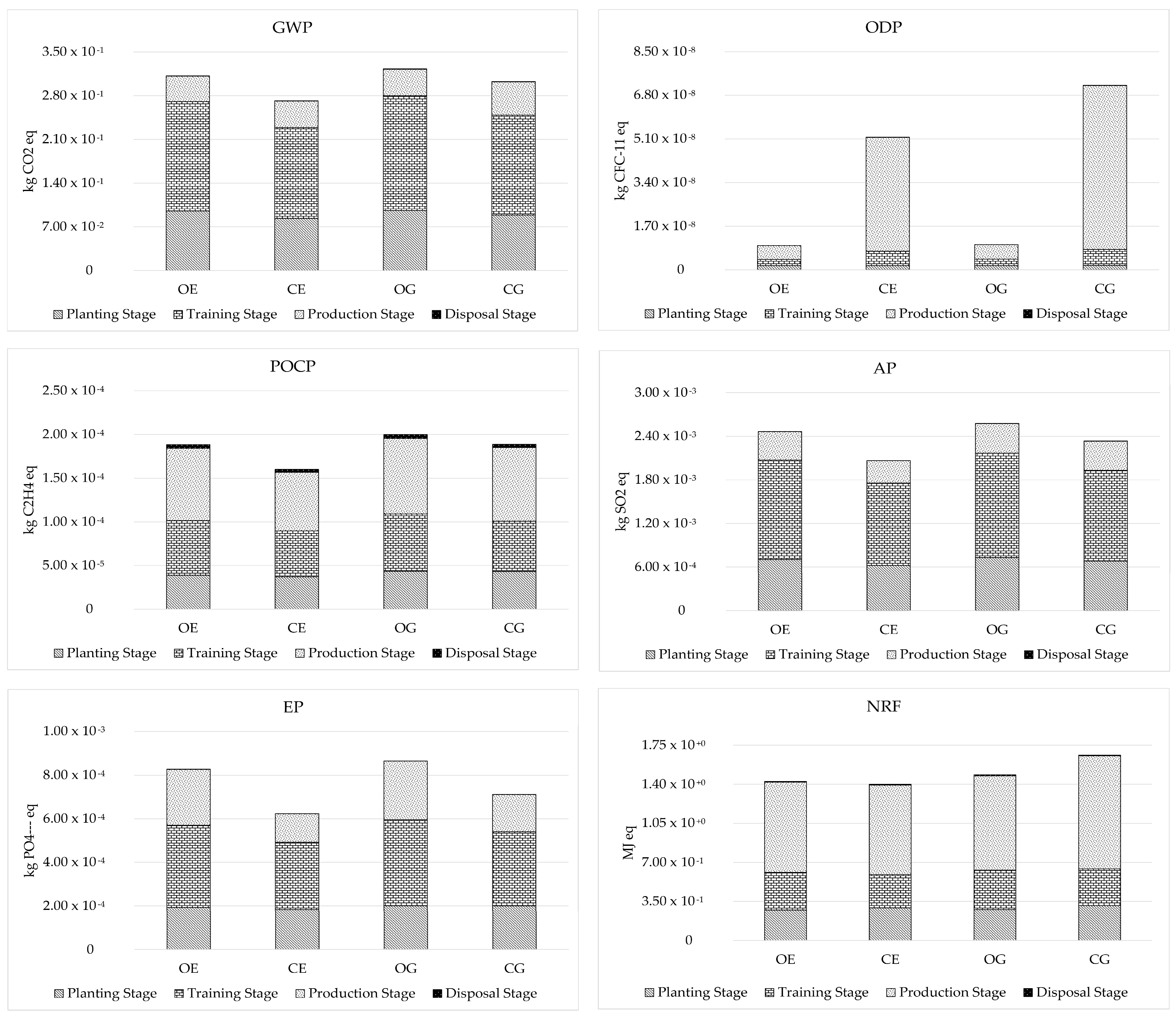
Results of EnLCIA are illustrated for each scenario by distinguishing the different stages of life cycle (Figure 3). In terms of GWP, the CE scenario shows the best performance, equal to 0.271 kg CO2 eq for one kg of grapes, attributed to Training Stage for 53% and to Planting Stage for 30%. For the same indicator (GWP), the worse result is attributable to OG scenario (0.329 kg CO2 eq), due to the greater influence of mechanical operation during the Production Stage. Acidification (AP) and Eutrophication (EP) impacts follow the same trend of GWP in terms of scenario performances. Regarding to Photochemical Oxidation (POCP), the Production Stage is most impacting (about 43%), followed by Training Stage (30%) and Planting Stage (20%), due to fuel combustion.
The impacts on Ozone layer Depletion Potential (ODP) are higher for the two conventional scenarios (CE, CG), due to pesticides use in production stage.
The impacts related to the use of Non Renewable Fossil (NRF) are similar for all scenarios, with only exception of CG that records a worse performance with a depletion of 1.66 MJ eq, 18% more impacting than CE scenario, due to the larger incidence of mechanical operations.
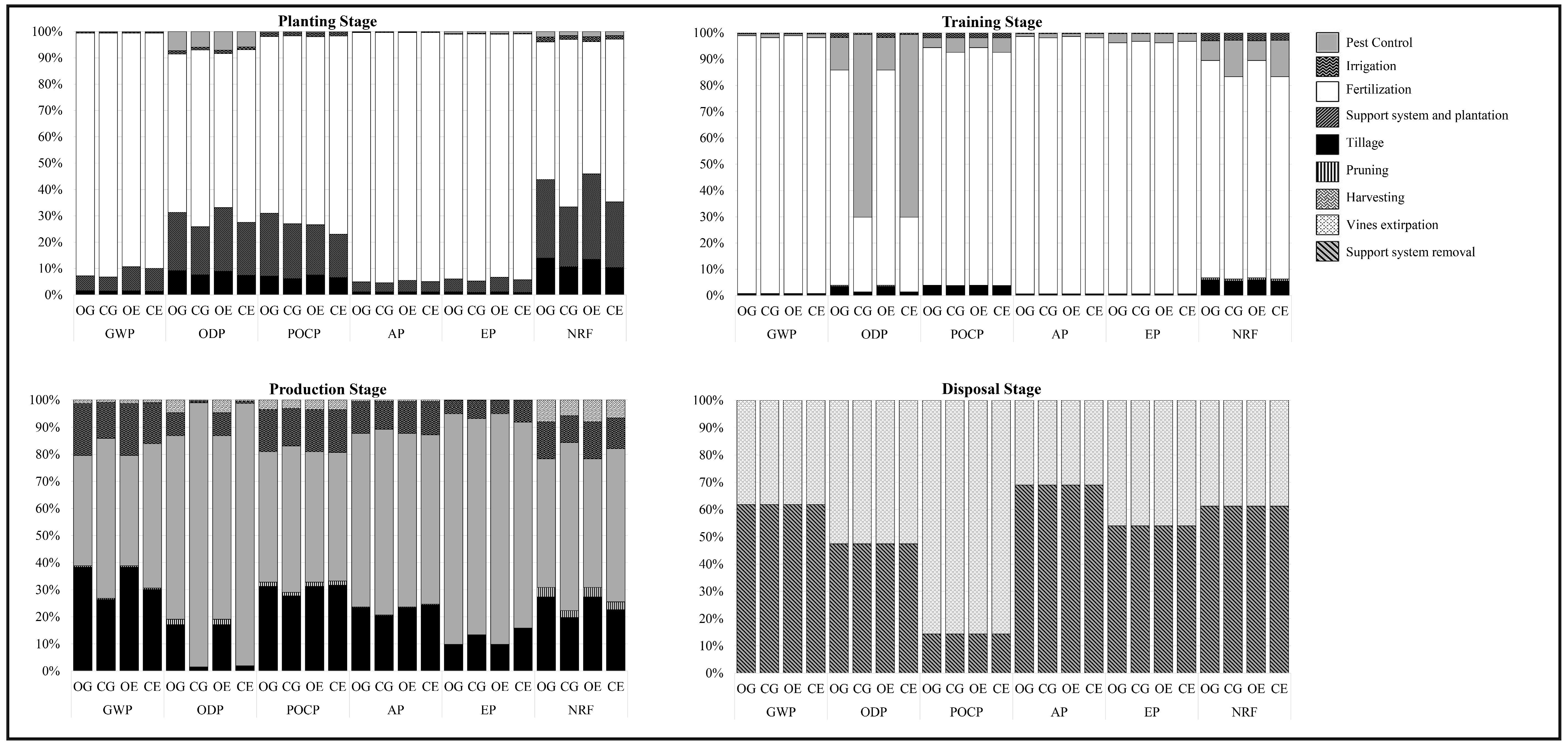
Concerning the environmental impacts of farming practices, LCA implementation shows different results for each life cycle stage (Figure 4). In Planting Stage, in all scenarios and for all indicators, the fertilization causes the most significant part of impacts, equal to about 90%.
For ODP, POCP and NRF impacts, the installation of support systems and plantation represents the second impacting farming operation, in particular due to the large use of metal and building material (e.g., concrete materials).
Training Stage shows similar incidence of farming operations impacts of the Planting Stage. Significant differences are in relation to ODP impacts category for which, in conventional scenarios, the pest control operations have greater incidence. In the production stage, the pest control represents, doubtless, the most impacting operation, followed by the tillage operations.
During the disposal stage (removal of support system and extirpation of plants), the impacts are caused by gasoil and gasoline combustion during removal operations.
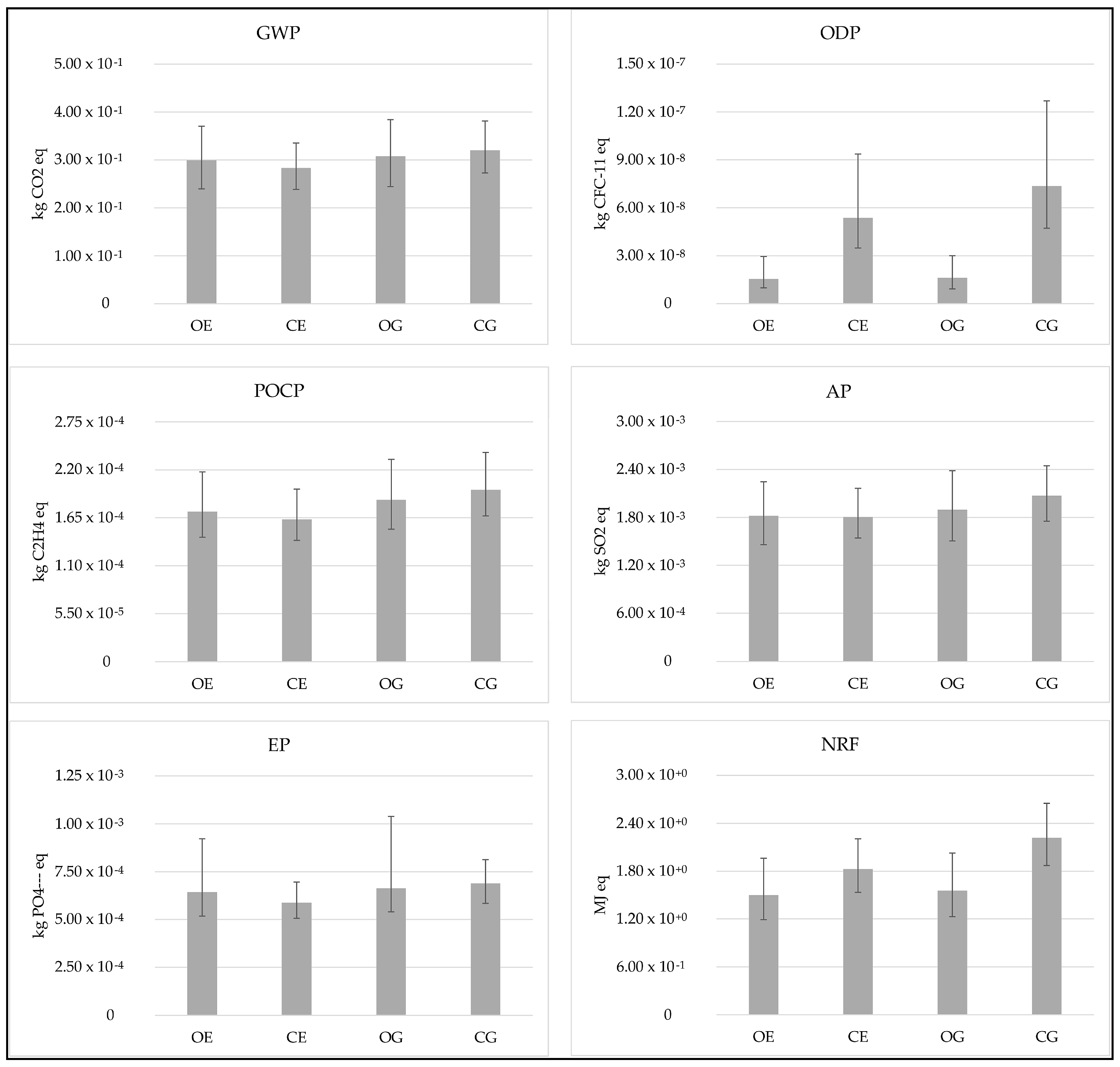
The sensitivity analysis performed through 1000-runs Monte Carlo simulation (Figure 5) allowed analyzing the uncertainty degree of results for each Impact Assessment Category, by considering the probability distribution of LCI parameters. Results of GWP, POCP, AP and NRF impact categories showed a lower uncertainty, as shown by the coefficients of variation in Table 5. On the contrary, ODP values have a lower confidence, as well as EP category, that showed a greater uncertainty for organic scenarios but lower for conventional ones.
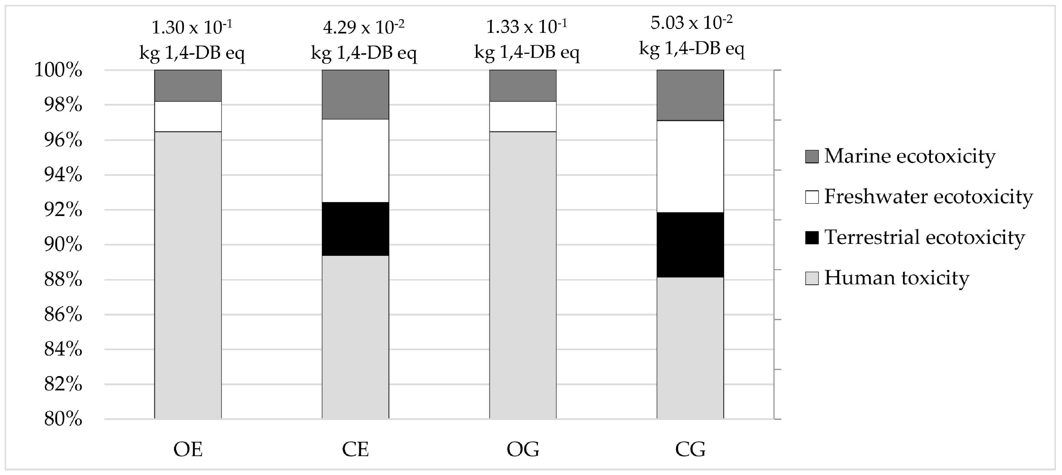
Toxicity indicators values are higher in organic scenarios and, in particular, HTP represents the most impacting category, accounting more than 90% of 1.4-dichlorobenzene eq kg−1 emissions. Pesticides production and emissions also represent the greatest contributor for TETP, MAETP and FAETP categories (Figure 6).
Conventional scenarios showed lower impacts related to toxicity indicators, thanks to smaller quantities of pesticides distributed and more homogeneous incidence among impact categories values. However, even in conventional scenarios, pesticides represent the most polluting factors with machineries production and usage. Regarding espalier (E) scenarios, the construction of supporting systems plays a relevant role in toxicity impacts.
Sensitivity analysis for the Toxicity Impact Assessment Categories showed a very high uncertainty degree, in particular concerning HTP in CG scenario (Table 6).
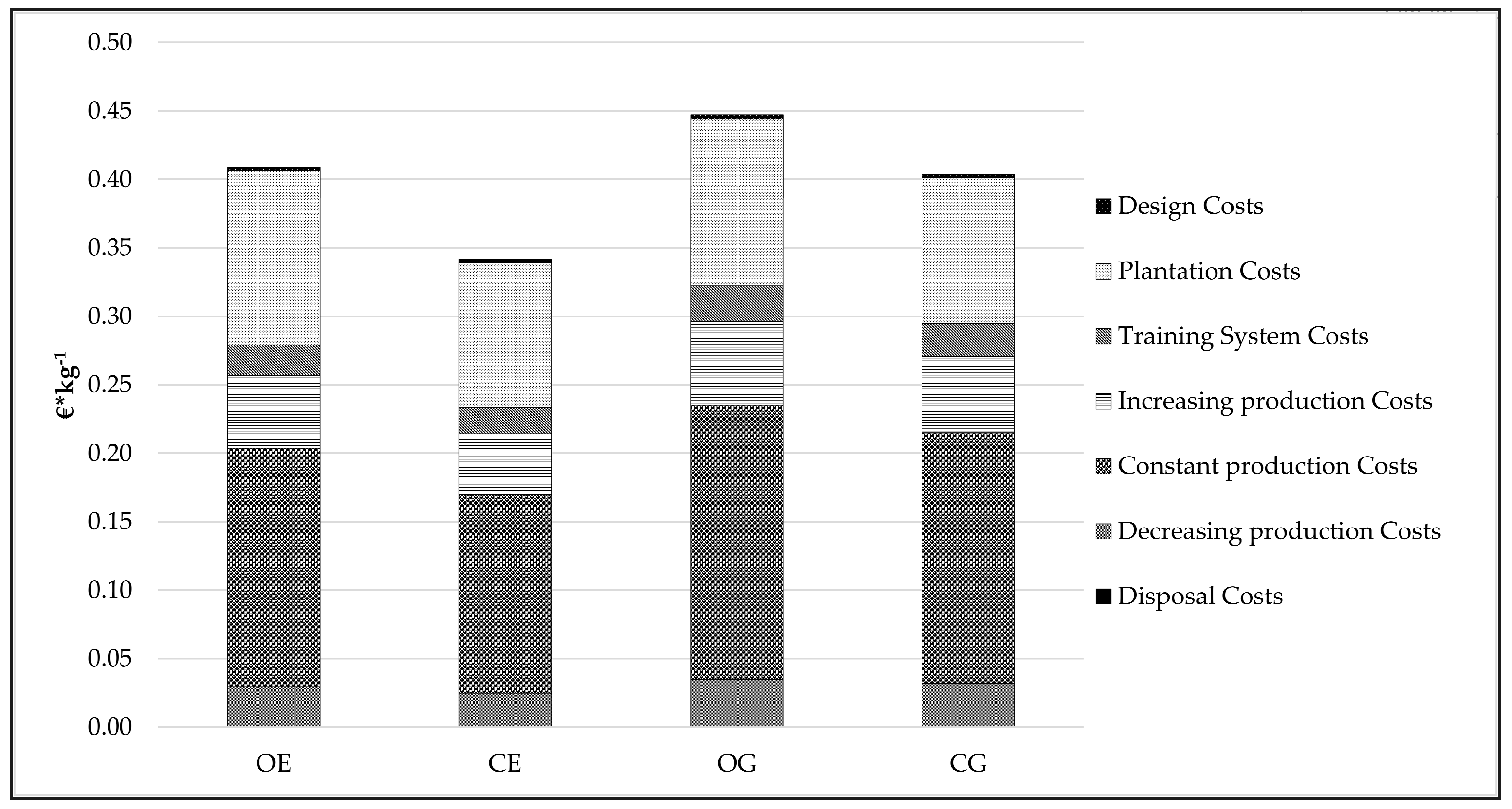
The LCC implementation has allowed to calculate all start-up, operating and disposal costs of each grapevine production system analyzed and for the whole life cycle.
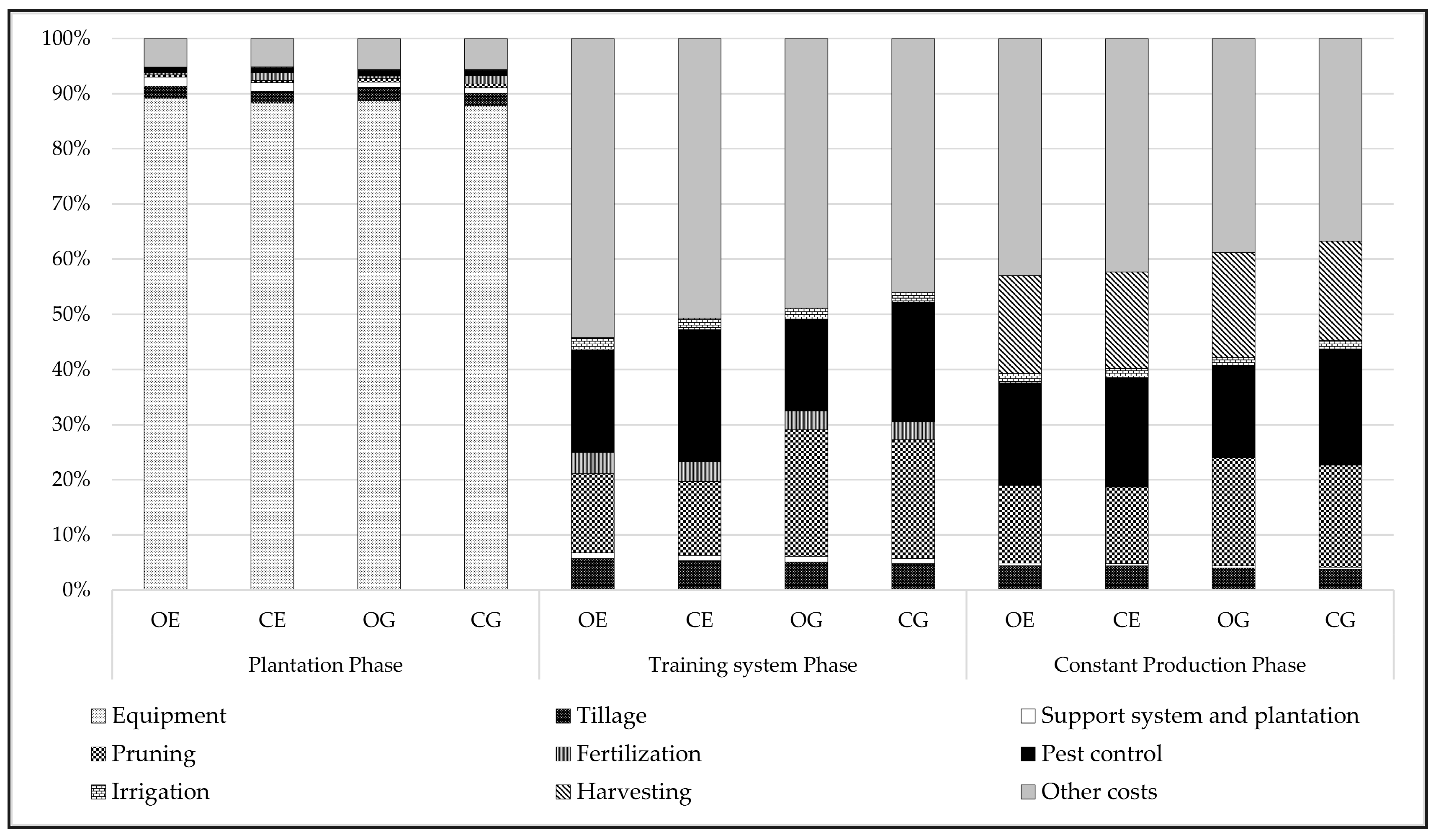
 Figure 7 and Figure 8 show for each scenario, in terms of FU, respectively the total life cycle costs for each stage and the operating costs for agricultural operations in the Production Stage, by including the expenses for materials, work and energy. The OG scenario represents the most expensive cultivation, with 0.447 € kg−1, followed by OE scenario (0.409 € kg−1). In both systems, the initial investment related to the Planting Stage and the constant Production Stage have the most impact. In more detail, for the same scenarios, the start-up costs are higher due to high purchase costs of raw materials and equipment. During the constant production stage, the higher operating costs are heavily influenced by both the harvesting and pruning operations (in terms of labor cost), and the pest control activities (in terms of input used). In contrast, the CE scenario registers the lower costs (0.342 € kg−1). However, with regard to the constant production stage, this scenario shows higher pest control costs than the organic scenarios.
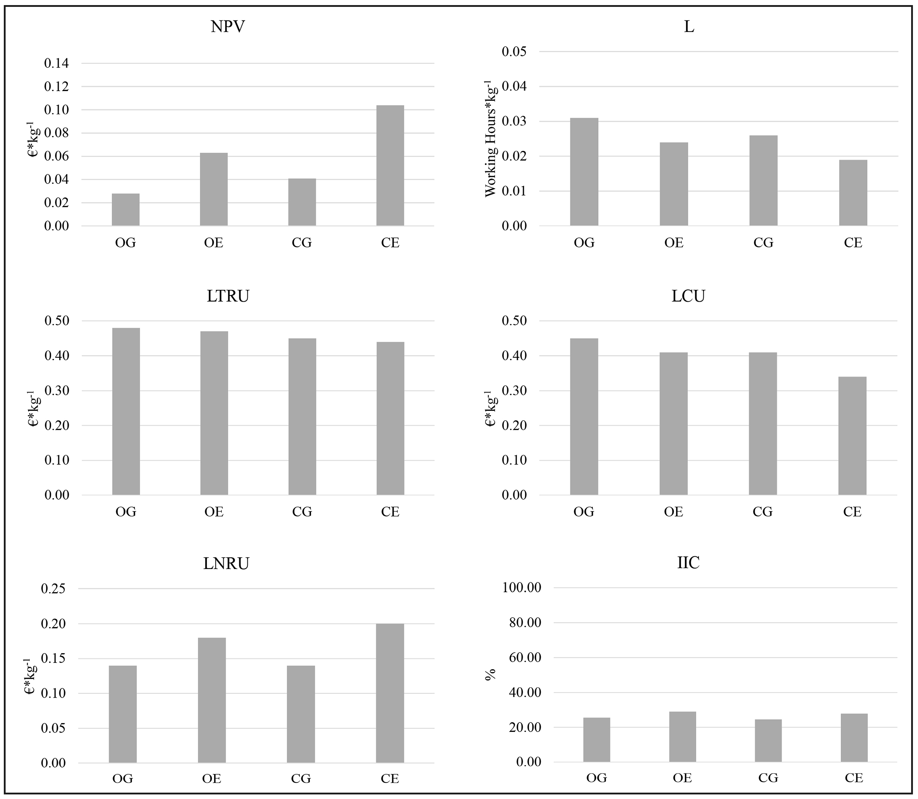
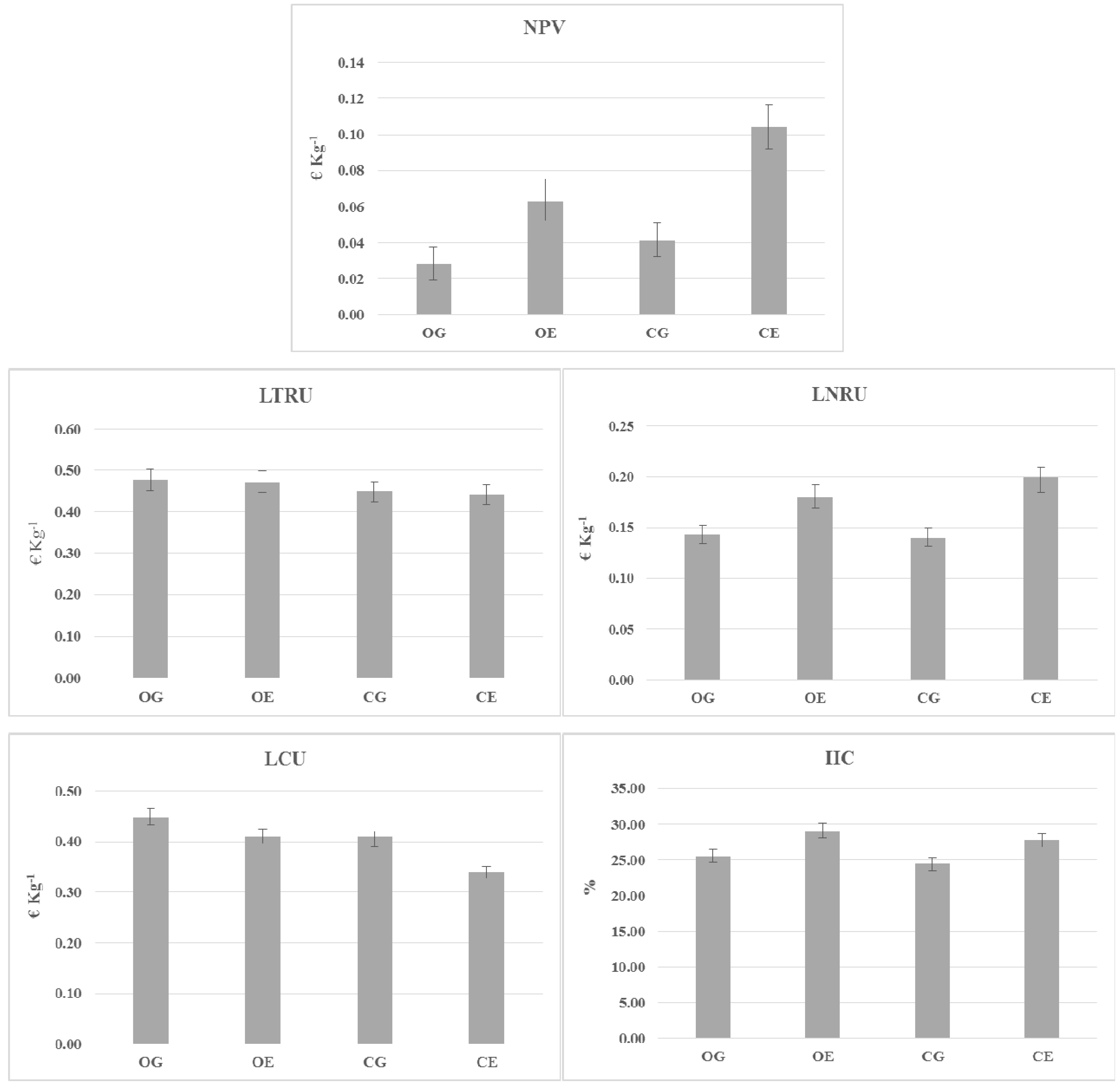
Figure 9 illustrates the results of economic indicators obtained from LCC analysis. The results show that the CE scenario realizes the better performances for all indicators examined, except for LTRU (Life Total Return Unit) and IIC (Initial Investment Cost), while the OG scenario shows the lowest performances, except for LTRU. More in detail, the NPV indicator, equal to 0.104 € kg−1 for CE scenario and to 0.028 € kg−1 for OG scenario, shows a greater investment profitability for the first scenario, due to the higher production yield than the organic system.
In terms of unit revenue (LTRU indicator), the CE and OG scenarios show opposite trends, with values of 0.44 € kg−1 and 0.48 € kg−1, respectively. At the same market prices, this is due to the greater subsidies to organic farms than the conventional systems. Regarding L (Labour per Production Unit) and LCU (Life Cost Unit) indicators, respectively equal to 0.019 € kg−1 and 0.34 € kg−1, the CE scenario achieves the best performances compared to OG scenario, due to the lowest incidence in terms of working hours and of total investment cost recorded by the conventional systems.
The sensitivity analysis on economic results was carried out by assuming a variation of ±0.4 p.p. of discount rate (Figure 10). The variation of discount rate generates a constant impact on all economic indicators and for each scenario, which was approximately between ±0.01 and ±0.03 € kg−1 for NPV, LCU, LTRU and LNRU and between ±0.9 and ±1.0 p.p. for IIC. In particular, a rate increase generates a negative effect on NPV, LTRU and LNRU, by influencing more negatively benefits than costs, due to the deferment of revenues in the case of simple investment.
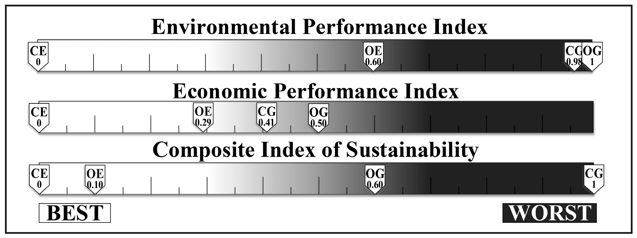
VIKOR results, in terms of Environmental Performance Index (EnPI), show that the scenarios with espalier training systems have better performances than gobelet training systems ones. Indeed, CE and OE scenarios are placed at the first two positions of the ranking, by recording, respectively, an EnPI equal to 0.00 and 0.60. The scenarios with gobelet training systems are less sustainable, because they are farther from the ideal condition; in particular, CG records a score of 0.98 while OG represents the anti-ideal scenario (EnPI equal to 1.0) (Figure 11). Furthermore, these results indicate that the conventional cropping systems are significantly better than organic ones.
Regarding the economic sustainability, the CE scenario, with an Economic Performance Index (EPI) equal to 0.00, is the closest to the ideal point, followed by OE scenario with a score of 0.29. In contrast, CG and OG scenarios have the worst performances accounting a score of 0.41 and 0.50, respectively. It follows that, similarly to the environmental results, scenarios with espalier training system have a better performance than gobelet ones and conventional systems are significantly better than organic ones.
Considering a concept of sustainability in a multidimensional perspective, results confirm that the scenario CE, with a Composite Index of Sustainability (CIS) equal to 0.00, identifies the best management strategy in terms of compromise between environmental impacts and economic ones, followed by OE scenario with a score of 0.12. Gobelet training systems scenarios are less sustainable; in particular, OG scenario records a score of 0.60, while CG represents the anti-ideal scenario with a distance equal to 1.00. It is interesting to notice that, only for the gobelet training system, does the organic cropping system record a better performance than conventional one.

5. Discussion

The results of the environmental analysis show that conventional scenarios reach generally better performances compared to organic ones. These findings are consistent with other studies [29,130], confirming that organic agriculture is not always the most suitable strategy from all point of views. In particular, the foremost issue, in the case of grapevine, is linked to the difference of yield between organic and conventional cultivation techniques (lower in the organic one) and therefore, the use of a mass FU favors the conventional scenarios [131]. The same aspect benefits espalier scenarios more than gobelet ones, the latter being less productive. However, also considering area based FU, organic production could be the worst, due to the nature of some inputs (e.g., pesticides and fertilizers such as sulphur and copper), which often cause significant impacts during their production phase and to the amount of product applied [29].
Nevertheless, the results of LCA might not be exhaustive for defining the environmental profile of an organic production because there are some environmental issues that cannot be assessed through an LCA. For example, organic farming, compared to conventional farming, increases biodiversity on a local scale, improves soil quality and increases the organic component of soils [29].
Global Warming Potential (GWP) impacts can be attributable to the higher incidence of CO2 eq emissions due to the use of mechanical operations, and the consequent diesel combustion, and to fertilization, confirming what observed by Neto et al. [43], Gazulla et al. [42] and Villanueva-Rey et al. [37]. This kind of results can be verified in conventional scenarios as well as in the organic ones, but with some differences. In fact, as showed in Figure 3, training and planting stages represent the most pollutant stages, in accordance with the study by Fusi et al. [31]; however, in the organic scenarios there are significant emissions during the production stage because of the larger use of mechanical operations (e.g., for weeding). This higher incidence in organic scenarios is in accordance with the findings by Villanueva-Rey et al. [37], relatively to biodynamic scenarios, endorsing also the results obtained by Point et al. [132] and Vázquez-Rowe et al. [48,53,133]. Overall, the organic scenarios obtain the worst results due to the lower productivity that causes the higher incidence of impacts per kg of product.
Findings showed that Ozone layer Depletion Potential (ODP) impacts are strictly connected with production stage that represents the highest influence (up to 88%). In more detail, this environmental impact (ODP) is linked with production of phytosanitary compounds, confirming also the findings by Neto et al. [43].
As expected, the impacts on Non Renewable Fossil (NRF) consumption arise mainly during the production stage and are connected to both fossil fuel consumption and chemicals production.
The detailed assessment of each agricultural life cycle stage of vine growing allowed us to understand the contribution of each stage to the eco-profile of grapevine and to highlight, in particular, the impacts generated during the unproductive stages, otherwise excluded from the analysis [29]. For example, it highlights the role of soil enrichment during the planting and the training stages. In all scenarios analyzed, fertilization represents only a temporary issue, being allowed only during unproductive stages [105]; nevertheless, it can be noticed that this operation represents a criticism. The large use of cow manure for basic fertilization enriches the soil and improves its structure, but a big part of nitrogen is lost in form of nitrous oxide and ammonia by volatilization and in form of nitrate by leaching [76].
The assessment of impacts related to the life cycle stages allowed us to underline the role that each agricultural operation plays in the vineyard eco-profile.
In the planting stage, the installation of support systems and plantation of tree represent the second most impacting operation in particular in terms of ODP, POCP and NRF indicators, due to the large use of metal and building materials (e.g., concrete materials), confirming the insights of Benedetto [45]. Probably, using recycled material for the construction of support structures would reduce the incidence of impacts in this stage.
The Training Stage shows, largely, a similar profile to the Planting Stage; however, the introduction, during the training stage, of pest control causes some significant differences in the ODP indicator.
In the Production Stage, the pest control represents the most pollutant for all impact categories. Indeed, during this stage there is a greater need for pest controls, in order to avoid loss of product. In particular, the control of Plasmopara viticola and Uncinula necator requires a constant monitoring and numerous applications of pesticides, producing high impacts due to the application and loss of active ingredients, to the use of distribution machines and to the emissions generated by diesel combustion [46]. The influence of machinery operations is confirmed by the results which show that the tillage practice represents the second most impacting operation in Production Stage [41], followed by the irrigation practice realized by tank truck.
The disposal stage entails a wider use of fossil fuels for removal of support systems and extirpation of plants, but, compared to the entire environmental life cycle performance, the incidence of this stage is minimal, while it represents an income from the economic profitability point of view.
The Monte Carlo analysis showed that environmental profiles are likely accurate for GWP, POCP, AP and NRF impact categories [50,125]; on the contrary, ODP values have a lower confidence, probably due to the higher uncertainty related to the statistical distribution of pesticide production data. The EP category showed variable results with a greater uncertainty for organic scenarios, but lower for conventional ones. Results are directly linked with statistical distribution of estimated emissions [124].
The assessment of toxicity impact showed higher values in organic scenarios, mainly due to the higher quantity of copper compounds emission in soil, confirming the studies the studies by Komárek et al. [134] and Neto et al. [43]. In conventional scenarios, even though the impacts are much lower, pesticides distribution represents once again the most polluting factors due to the incidence of the machineries production and their use during production stage [43,132]. Focusing on the espalier scenarios, the large use of metal materials for the construction of supporting systems generates a significant share of impacts [37,43]. The very high uncertainty degree shown through the sensitivity analysis makes inconsistent the obtained results; however, they can be useful as indicative values [124].
The LCC results strictly depended on production yield, that was higher in the conventional cropping systems than organic ones, and on training systems, more difficult to manage for the gobelet system than espalier ones, although these latter entailed higher initial investments. Moreover, the findings were related to the assumption of a price invariance during the reference period [75].
Because of the above-mentioned aspects, the organic grapevine production systems, compared to conventional ones, reached the worst performance. Along the whole vineyard life cycle, the major economic hotspots were found in the planting stage, due to the higher plantation costs in term of raw material and equipment, and in the constant production stage because of the higher operating costs (in terms of both labor costs for harvesting and pruning operations, and pest control costs).
The manual grape harvesting and cane pruning were costly due to the high human labor requirements. Although the mechanical grape harvest can represent a way to reduce costs and improve profit margins [83], the vine growers interviewed affirmed to prefer the manual harvesting for ensuring a high-quality wine production. For the same reasons, the vine growers preferred the manual cane pruning, which permitted a better balancing between fruiting and vegetative buds and a higher quality production compared to mechanized pruning. Moreover, the existent vineyard structure is not suitable for performing a mechanical pruning, which involves specific characteristics in terms of training system, vegetation density, quantity of shoots and length of the rows. Mechanical pruning can be cost-effective and more practical where the vegetation is more extensive and the quantity of shoots is higher, together with an adequate row length [135].
In a sustainability assessment context, further comparison between different mechanical harvesting and pruning scenarios can be examined, in order to identify the most appropriate scenario not only in economic terms but also in environmental ones.
The high economic impact for pest control in the organic systems is caused by the major use of input and number of treatments; while in the conventional ones is due to the higher market price of phytoiatric products. An efficient use of these inputs would be suitable in all grapevine systems for reducing operating costs.
In terms of profitability, the conventional-espalier (CE) grapevine cultivation is considered the most profitable investment due to the higher production yield and the lower costs than the other systems. Overall, it is noteworthy that all scenarios are strongly dependent from European subsidies, with the exception of the CE scenario whose investments could be profitable also without public financing [40,80].
The VIKOR technique has allowed identifying the compromise solution between the four selected scenarios. The CE scenario represents the most sustainable from both environmental and economic perspectives (considered alone and integrated together), followed by the OE system. This latter showed, in the environmental performance index and in the economic one, a closer position to the worst solution, while considering the composite index of sustainability it is near to the ideal solution. These kind of results highlight that it is not enough to analyze individually the different sustainability dimensions, and confirm that it is necessary to make an integrated analysis to identify the most suitable compromise in real decision-making problems.
The environmental indicators used in this work were selected according to EPD Certification. Therefore, the findings can suggest practical implications useful for entrepreneurs as well as for consumers. The former can improve and certify the environmental profile of their products and therefore increase the added value to reach market segments that are aware of sustainable production so, potentially, willing to pay a premium price. The latter can satisfy their sensibility to the environment protection by having more knowledge on the impacts of different production systems. In this study, the environmental improvement is complementary to economic performances. The economic indicators are more oriented to the farmers, who can use them to evaluate and improve their businesses. The utilization of environmental and economic indicators different from those applied in this study, could probably change the final rank and the decision-makers/stakeholders perspectives. The use of a synthetic index allows a more understandable reading of results and then a simpler measure of sustainability [20,21].
Making a general consideration for future researches, in order to improve at the same time the environmental and economic hotspots of products life cycles an iterative improvement process, as it is the combination of Life Cycle tools and MCDA, would be suitable [93,94,95,96]. However, it should be taken into account that the final rank would be obviously connected to the choice of the FU, as well as to the eventual assignment of weights to the different dimensions. Specifically, this latter aspect is strictly connected to different perspectives of involved stakeholders. The indicators selection also influences the rank and the definition of the compromise solution.

6. Conclusions

This paper has examined a specific issue concerning the environmental and economic sustainability of grapevine production systems applying LCA and LCC methodologies in order to identify their main hotspots and to select the most sustainable and appropriate scenarios through a MCDA method. The advantages obtained from the proposed methodology concern finding the compromise between environmental and economic expectations, and obtaining a tool to accompany processes of decision-making considering multiple criteria by means of a MCDA technique. In particular, the two-dimensional sustainability approach based on a joint implementation of LCA, LCC and VIKOR technique allowed us to overcome the constraints existing in single perspective-based approaches. The aggregation of conflicting indicators (environmental and economic) by means of mono-dimensional indices and multiple ones, allowed additional ranking of the alternative scenarios of sustainability. It is clear that this study is not able of encompass the whole sustainability from a multi-stakeholder perspective, due to the lack of the social aspects assessment and to the choice of environmental and economic indicators more oriented to farmers.
Accepting the present two-dimensional sustainability evaluation, this method could be useful to be applied to others products; moreover, the MCDA method would allow attributing different weights to sustainability dimensions reflecting the perspectives of possible stakeholders involved. Therefore, this work mainly provides useful information for corporate decision-making processes in order to decrease the environmental burdens and cost factors, improving agricultural management practices through a more efficient use of farm inputs. Moreover, the results may positively satisfy environmental conscious consumers.
The results showed that the conventional practices associated to espalier training system are a more sustainable strategy, from both the environmental and economic points of view. However, the findings are obviously influenced by choices made during the methodologies implementation. Firstly, the different yield between conventional and organic cultivation techniques (lower in the organic ones) certainly affected the result, especially due to the FU used (1 kg of grapes). Furthermore, these results could not be exhaustive disregarding some environmental and economic benefits generated from organic farming such as the increase of biodiversity, soil quality improvement and the increase of the organic components of soils.
The extension of the system boundary of the agricultural phase by including the unproductive stages enabled the understanding of some significant hotspots, which otherwise would not be taken into account as the fertilization, and/or the building of the support systems. The choice to carry out this extension has also led to the necessity to make some choice in order to model the vineyard life cycle. However, this extension also introduces an amplification in the uncertainty of data, which should be considered, but it is nevertheless preferable to the oversimplification by considering only productive stage.
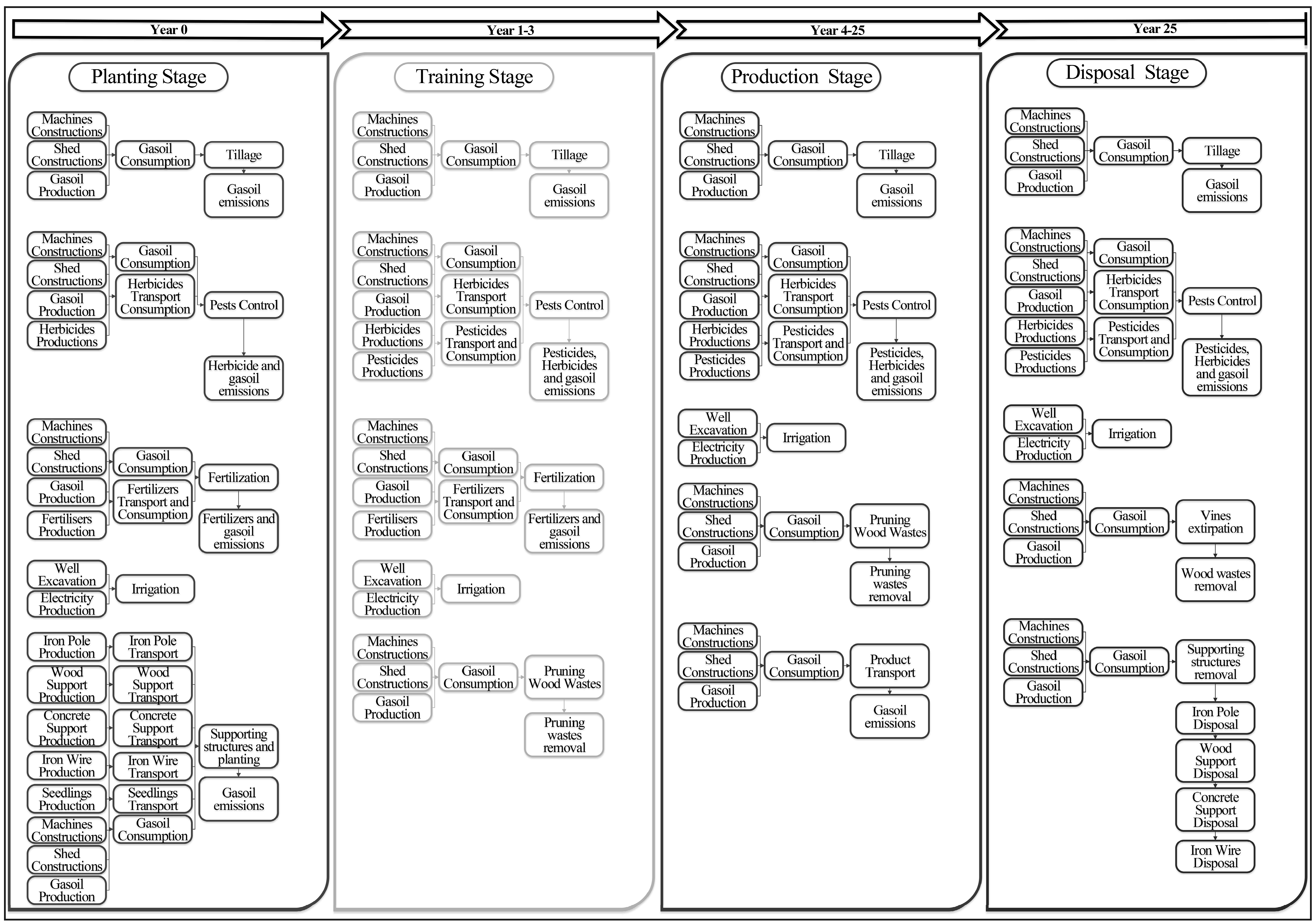
The long term (25 years) vineyard modelling certainly introduces some limitations such as the difficulty to foresee singular events that could greatly affect the management techniques or regulations changes (for example, a new norm could forbid the use of some products for pest management). Analyzing companies already in full production stage can bring limitations; but they could be overcame improving the quality of past data (previous to full production phase of the vineyard) and conducting sensitivity analyses on the future stages (from the current stage to disposal). Unfortunately, these options are not always viable because of the high engagement in terms of time and costs, both in the data gathering and in the computational phase.
A further limitation of the study was the lack of a whole adaptation of the computational structures between LCA and LCC analysis.
The implementation of the two life cycle methods was carried out adopting a common database, keeping the same FU and system boundaries and assessing in monetary terms the physical flows of the life cycle inventory. Even if it represents the most adopted approach by several researchers, it is still necessary to make remarkable efforts for the alignment of the computational structures of LCA and LCC.
From an economic point of view, a further limitation concerned the assumption of invariance of the price during the reference period; in other words, this economic analysis did not contemplate possible market dynamics. Therefore, an uncertainty analysis of the LCC results considering price variability would be suitable.
Further research advances could be related to the consideration of all these issues in order to improve the quality of results, contributing to provide the best sustainable compromise in wine supply chains.

Supplementary Files

Supplementary File 1

Acknowledgments

This research is funded by the Italian Ministry of University and Research (MIUR) within the research project: Distretto ad alta tecnologia agroindustrale della Calabria AGRIFOODTECH (PON03PE_00090_3) “Modelli sostenibili e nuove tecnologie per la valorizzazione delle filiere vegetali mediterranee”.

Author Contributions

The individual contribution and responsibilities of the authors were as follows: Giacomo Falcone contributed to research design, implemented the L.C.A. methodology and wrote Section 3.3; Teodora Stillitano contributed to research design, implemented the L.C.C. methodology and wrote Section 3.4; Anna Irene De Luca contributed to research design, wrote Section 1 and Section 3.5 and helped to draft edit and revise the whole manuscript; Giuseppa Romeo elaborated VIKOR technique; Alfio Strano designed research and wrote Section 1 and Section 3.1; Giovanni Gulisano is the research coordinator; Section 2, Section 3.2, Section 4, Section 5 and Section 6 were a team task. All authors have read and approved the final manuscript.

Conflicts of Interest

The authors declare no conflict of interest.

References

  1. Weil, R.R. Defining and using the concept of sustainable agriculture. J. Agron. Educ. 1990, 19, 126–130. [Google Scholar]
  2. De Luca, A.I.; Molari, G.; Seddaiu, G.; Toscano, A.; Bombino, G.; Ledda, L.; Milani, M.; Vittuari, M. Multidisciplinary and innovative methodologies for sustainable management in agricultural systems. Environ. Eng. Manag. J. 2015, 14, 1571–1581. [Google Scholar]
  3. Kajikawa, Y.; Tacoa, F.; Yamaguchi, K. Sustainability science: The changing landscape of sustainability research. Sustain. Sci. 2014, 9, 431–438. [Google Scholar] [CrossRef]
  4. European Commission. Communication from the Commission EUROPE 2020: A Strategy for Smart, Sustainable and Inclusive Growth; COM (2010) 2020; European Commission: Brussels, Belgium, 2010. [Google Scholar]
  5. Beccali, M.; Cellura, M.; Iudicello, M.; Mistretta, M. Resource consumption and environmental impacts of the agrofood sector: Life cycle assessment of Italian citrus-based products. Environ. Manag. 2009, 43, 707–724. [Google Scholar] [CrossRef] [PubMed]
  6. EEA (European Environment Agency). Annual European Community Greenhouse Gas Inventory Report 2014; Version 27; Technical Report No. 9; Submission to the UNFCCC Secretariat 2014; EEA: Copenhagen, Denmark, 2014. [Google Scholar]
  7. EEA. Environmental Indicator Report 2012—Ecosystem Resilience and Resource Efficiency in a Green Economy in Europe; EEA: Copenhagen, Denmark, 2012. [Google Scholar]
  8. San Cristóbal, J.R. Multi-criteria decision-making in the selection of a renewable energy project in Spain: The Vikor method. Renew. Energy 2011, 36, 498–502. [Google Scholar] [CrossRef]
  9. Mariani, A.; Vastola, A. Sustainable winegrowing: Current perspectives. Int. J. Wine Res. 2015, 7, 37–48. [Google Scholar] [CrossRef]
  10. Sogari, G.; Corbo, C.; Macconi, M.; Menozzi, D.; Mora, C. Consumer attitude towards sustainable-labelled wine: An exploratory approach. Int. J. Wine Bus. Res. 2015, 27, 312–328. [Google Scholar] [CrossRef]
  11. OIV Guidelines for Sustainable Vitiviniculture: Production, Processing and Packaging of Products, CST 1-2008. Available online: http://www.oiv.int/public/medias/2089/cst-1-2008-en.pdf (accessed on 18 May 2016).
  12. Guinée, J.B. (Ed.) Handbook on Life Cycle Assessment—Operational Guide to the ISO Standards; Kluwer Academic Publishers: Dordrecht, The Netherlands, 2002.
  13. Remmen, A.; Jensen, A.A.; Frydendal, J. Life Cycle Management—A Business Guide to Sustainability; UNEP and Danish Standards; United Nations Environment Programme (UNEP): Nairobi, Kenya, 2007. [Google Scholar]
  14. International Organization for Standardization. ISO 14040:2006 Environmental Management—Life Cycle Assessment—Principles and Framework; International Organization for Standardization (ISO): Geneva, Switzerland, 2006. [Google Scholar]
  15. International Organization for Standardization. ISO 14044:2006 Environmental Management—Life Cycle Assessment—Requirements and Guidelines; International Organization for Standardization (ISO): Geneva, Switzerland, 2006. [Google Scholar]
  16. International Organization for Standardization. ISO 15686-5:2008 Buildings and Constructed Assets-Service Life Planning-Life Cycle Costing; International Organization for Standardization (ISO): Geneva, Switzerland, 2008. [Google Scholar]
  17. De Luca, A.I.; Iofrida, N.; Strano, A.; Falcone, G.; Gulisano, G. Social life cycle assessment and participatory approaches: A methodological proposal applied to citrus farming in Southern Italy. Integr. Environ. Assess. Manag. 2015, 11, 383–396. [Google Scholar] [CrossRef] [PubMed]
  18. Linkov, I.; Satterstrom, F.K.; Kiker, G.; Batchelor, C.; Bridges, T.; Ferguson, E. From comparative risk assessment to multi-criteria decision analysis and adaptive management: Recent developments and applications. Environ. Int. 2006, 32, 1072–1093. [Google Scholar] [CrossRef] [PubMed]
  19. Linkov, I.; Seager, T. Coupling multi-criteria decision analysis, life cycle assessment and risk assessment for emerging threats. Environ. Sci. Technol. 2011, 45, 5068–5074. [Google Scholar] [CrossRef] [PubMed]
  20. De Luca, A.I.; Romeo, G.; Falcone, G.; Stillitano, T.; Strano, A. Una metodologia multicriteriale per la valutazione integrata della sostenibilità di sistemi produttivi cerealicoli. In Proceedings of the VIII Convegno Scientifico Dell’Associazione Rete Italiana LCA I Nuovi Orizzonti dell’LCA: Verso un Approccio Sistemico e Integrato Alla Progettazione di Prodotti, Processi e Servizi, Firenze, Italy, 19–20 June 2014; Scalbi, S., Dominici Lopireno, A., Eds.; Enea Agenzia Nazionale per le Nuove Tecnologie: Rome, Italy, 2014; pp. 8–14. [Google Scholar]
  21. Falcone, G.; De Luca, A.I.; Romeo, G.; Stillitano, T.; Strano, A.; Gulisano, G. Integrated sustainability assessment of agricultural processes using the multi-criteria technique vikor. In Proceedings of the Ecomondo 19a Fiera Internazionale dello Sviluppo Sostenibile, Rimini, Italy, 5–8 November 2014.
  22. Ren, J.; Manzardo, A.; Mazzi, A.; Zuliani, F.; Scipioni, A. Prioritization of bioethanol production pathways in China based on life cycle sustainability assessment and multicriteria decision-making. Int. J. Life Cycle Assess. 2015, 20, 842–853. [Google Scholar] [CrossRef]
  23. Ayman, M.M. Performance Evaluation and Improvement Technique for Organizations. Master’s Thesis, Fayoum University, Fayoum, Egypt, 2014. [Google Scholar]
  24. Opricovic, S. A compromise solution in water resources planning. Int. Ser. Prog. Wat. Res. 2009, 23, 1549–1561. [Google Scholar] [CrossRef]
  25. De Luca, A.I.; Falcone, G.; Iofrida, N.; Stillitanto, T.; Strano, A.; Gulisano, G. Life cycle methodologies to improve agri-food systems sustainability. Riv. Studi Sulla Sosten. 2015, 1, 135–150. [Google Scholar] [CrossRef]
  26. Notarnicola, B.; Salomone, R.; Petti, L.; Renzulli, P.A.; Roma, R.; Cerutti, A.K. (Eds.) Life Cycle Assessment in the Agri-Food Sector Case Studies, Methodological Issues and Best Practices; Springer: Basel, Switzerland, 2015.
  27. Poritosh, R.; Daisuke, N.; Takairo, O.; Qingyi, X.; Hiroshi, O.; Nobutaka, N.; Takeo, S. A review of Life Cycle Assessment (LCA) on some food products. J. Food Eng. 2009, 90, 1–10. [Google Scholar]
  28. Sanjuan, N.; Ubeda, L.; Clemente, G.; Mulet, A.; Girona, F. LCA of integrated orange production in the Comunidad Valenciana (Spain). Int. J. Agric. Resour. Gov. Ecol. 2005, 4, 163–177. [Google Scholar] [CrossRef]
  29. Petti, L.; Arzoumanidis, I.; Benedetto, G.; Bosco, S.; Cellura, M.; De Camillis, C.; Fantin, V.; Masotti, P.; Pattara, C.; Raggi, A.; et al. Life cycle assessment in the wine sector. In Life Cycle Assessment in the Agri-Food Sector Case Studies, Methodological Issues and Best Practices; Notarnicola, B., Salomone, R., Petti, L., Renzulli, P.A., Roma, R., Cerutti, A.K., Eds.; Springer International Publishing: Basel, Switzerland, 2015; pp. 123–184. [Google Scholar]
  30. Arzoumanidis, I.; Petti, L.; Raggi, A.; Zamagni, A. Life Cycle Assessment (LCA) for the Agri-Food Sector. In Product-Oriented Environmental Management System (POEMS)—Improving Sustainability and Competitiveness in the Agri-Food Chain with Innovative Environmental Management Tools; Salomone, R., Clasadonte, M.T., Proto, M., Raggi, A., Eds.; Springer International Publishing: Dordrecht, The Netherlands, 2013; pp. 105–122. [Google Scholar]
  31. Pattara, C.; Cichelli, A.; Civitarese, C.; Di Martino, M. A comparison of carbon footprints in wine production: The case of two cooperative wineries in central Italy. Bull. L’OIV 2012, 85, 307–316. [Google Scholar]
  32. Petti, L.; Ardente, F.; Bosco, S.; De Camillis, C.; Masotti, P.; Pattara, C.; Raggi, A.; Tassielli, G. In stato dell’arte della Life Cycle Assessment (LCA) nel comparto vitivinicolo. In Proceedings of the Scientific Convention of Rete Italiana LCA “La Metodologia LCA: Approccio Proattivo per le Tecnologie Ambientali. Casi Studio ed esperienze Applicative”, Padova, Italy, 22 April 2010.
  33. Barberini, M.; Cecchini, F.; Della Giovanpaola, M.; Franchini, F.; Mangani, F.; Neri, P.; Parmeggiani, G.; Tosi, M. Analisi del Ciclo di Vita del Vino: Confronto tra la Produzione Convenzionale e Quella Biologica. Master’s Thesis, Università di Urbino and ENEA, Urbino, Italy, 2004. [Google Scholar]
  34. Cecchini, F.; Neri, P.; Franchini, F.; Catto, G.; Feoli, E.; Altobelli, A. Analisi Ambientale Della Filiera Vitivinicola del Cabernet Sauvignon in Friuli Venezia Giulia Secondo il Metodo LCA. Master’s Thesis, Università Degli Studi di Trieste and ENEA, Trieste, Italy, 2005. [Google Scholar]
  35. Kavargiris, S.E.; Mamolos, A.P.; Tsatsarelis, C.A.; Nikolaidou, A.E.; Kalburtji, K.L. Energy resources’ utilization in organic and conventional vineyards: Energy flow, greenhouse gas emissions and biofuel production. Biomass Bioenergy 2009, 33, 1239–1250. [Google Scholar] [CrossRef]
  36. Niccolucci, V.; Galli, A.; Kitzes, J.; Pulselli, R.M.; Borsa, S.; Marchettini, N. Ecological footprint analysis applied to the production of two Italian wines. Agric. Ecosyst. Environ. 2008, 128, 162–166. [Google Scholar] [CrossRef]
  37. Villanueva-Rey, P.; Vázquez-Rowe, I.; Moreira, M.T.; Feijoo, G. Comparative Life Cycle Assessment in the wine sector: Biodynamic vs. conventional viticulture activities in NW Spain. J. Clean. Prod. 2014, 65, 330–341. [Google Scholar] [CrossRef]
  38. Fusi, A.; Guidetti, R.; Benedetto, G. Delving into the environmental aspect of a Sardinian white wine: From partial to total life cycle assessment. Sci. Total Environ. 2014, 472, 989–1000. [Google Scholar] [CrossRef] [PubMed]
  39. Arcese, G.; Lucchetti, M.C.; Martucci, O. Analysis of sustainability based on Life Cycle Assessment: An empirical study of wine production. J. Environ. Sci. Health B 2012, 1, 682–689. [Google Scholar]
  40. Strano, A.; De Luca, A.I.; Falcone, G.; Iofrida, N.; Stillitano, T.; Gulisano, G. Economic and environmental sustainability assessment of wine grape production scenarios in Southern Italy. Agric. Sci. 2013, 4, 12–20. [Google Scholar] [CrossRef]
  41. Ardente, F.; Beccali, G.; Cellura, M.; Marvuglia, A. POEMS: A case study of an Italian wine-producing firm. Environ. Manag. 2006, 38, 350–364. [Google Scholar] [CrossRef] [PubMed]
  42. Gazulla, C.; Raugei, M.; Fullana-i-Palmer, P. Taking a life cycle look at crianza wine production in Spain: Where are the bottlenecks. Int. J. Life Cycle Assess. 2010, 15, 330–337. [Google Scholar] [CrossRef]
  43. Neto, B.; Dias, A.C.; Machado, M. Life Cycle Assessment of the supply chain of a Portuguese wine: From viticulture to distribution. Int. J. Life Cycle Assess. 2013, 18, 590–602. [Google Scholar] [CrossRef]
  44. Notarnicola, B.; Tassielli, G.; Nicoletti, G.M. Life cycle assessment (LCA) of wine production. In Environmentally-Friendly Food Processing; Mattsonn, B., Sonesson, U., Eds.; Woodhead Publishing Limited: Cambridge, UK, 2003; pp. 306–326. [Google Scholar]
  45. Benedetto, G. The environmental impact of a Sardinian wine by partial life cycle assessment. Wine Econ. Policy 2013, 2, 33–41. [Google Scholar] [CrossRef]
  46. Bosco, S.; Massai, R.; Di Bene, C.; Bonari, E.; Galli, M.; Remorini, D. Greenhouse gas emissions in the agricultural phase of wine production in the Maremma rural district in Tuscany, Italy. Ital. J. Agron. 2011, 6, 93–100. [Google Scholar] [CrossRef] [Green Version]
  47. Cerutti, A.K.; Beccaro, G.L.; Bosco, S.; De Luca, A.I.; Falcone, G.; Fiore, A.; Iofrida, N.; Lo Giudice, A.; Strano, A. Life Cycle Assessment in the Fruit Sector. In Life Cycle Assessment in the Agri-Food Sector Case Studies, Methodological Issues and Best Practices; Notarnicola, B., Salomone, R., Petti, L., Renzulli, P.A., Roma, R., Cerutti, A.K., Eds.; Springer: Cham, Switzerland, 2015; pp. 333–388. [Google Scholar]
  48. Vázquez-Rowe, I.; Villanueva-Rey, P.; Iribarren, D.; Moreira, M.T.; Feijoo, G. Joint life cycle assessment and data envelopment analysis of grape production for vinification in the Rías Baixas appellation (NW Spain). J. Clean. Prod. 2012, 27, 92–102. [Google Scholar] [CrossRef]
  49. BIER (Beverage Industry Environmental Roundtable). Research on the Carbon Footprint of Wine. Available online: http://media.wix.com/ugd/49d7a0_4d74ddfdfbd64d3a8c1b27c17f460e36.pdf (accessed on 8 August 2016).
  50. Bosco, S.; Di Bene, C.; Galli, M.; Remorini, D.; Massai, R.; Bonari, E. Soil organic matter accounting in the carbon footprint analysis of the wine chain. Int. J. Life Cycle Assess. 2013, 18, 973–989. [Google Scholar] [CrossRef]
  51. Soosay, C.; Fearne, A.; Dent, B. Sustainable value chain analysis – a case study of Oxford Landing from “vine to dine”. Supply Chain Manag. Int. J. 2012, 17, 68–77. [Google Scholar]
  52. Pattara, C.; Raggi, A.; Cichelli, A. Life Cycle Assessment and carbon footprint in the wine supply-chain. Environ. Manag. 2012, 49, 1247–1258. [Google Scholar] [CrossRef] [PubMed]
  53. Vázquez-Rowe, I.; Rugani, B.; Benetto, E. Tapping carbon footprint variations in the European wine sector. J. Clean. Prod. 2013, 43, 146–155. [Google Scholar] [CrossRef]
  54. Ene, S.A.; Teodosiu, C.; Robu, B.; Volf, I. Water footprint assessment in the winemaking industry: A case study for a Romanian medium size production plant. J. Clean. Prod. 2013, 43, 122–135. [Google Scholar] [CrossRef]
  55. Pina, L.; Dias, A.; Neto, B.; Arroja, L.; Quinteiro, P. The water footprint of wine production in Portugal: A case study on vinho verde. In Proceedings of the Poster Session 6th International Conference on Industrial Ecology (ISIE 2011 Conference), Berkeley, CA, USA, 7–10 June 2011.
  56. Klöpffer, W. Life cycle sustainability assessment of products. Int. J. Life Cycle Assess. 2008, 13, 89–95. [Google Scholar] [CrossRef]
  57. Swarr, T.E.; Hunkeler, D.; Klöpffer, W.; Pesonen, H-L.; Ciroth, A.; Brent, A.C.; Pagan, R. Environmental life cycle costing: A code of practice. Int. J. Life Cycle Assess. 2011, 16, 389–391. [Google Scholar] [CrossRef]
  58. Dhillon, B.S. Life Cycle Costing: Techniques, Models, and Applications; Gordon and Breach Science Publishers: New York, NY, USA, 1989. [Google Scholar]
  59. Gluch, P.; Baumann, H. The life cycle costing (LCC) approach: A conceptual discussion of its usefulness for environmental decision-making. Build. Environ. 2004, 39, 571–580. [Google Scholar] [CrossRef]
  60. Huppes, G.; van Rooijen, M.; Kleijn, R.; Heijungs, R.; de Koning, A.; van Oers, L. Life Cycle Costing and the Environment; Report of a project commissioned by the Ministry of VROM-DGM for the RIVM Expertise Centre LCA; Ministry of Housing, Spatial, Planning and the Environment (VROM): Den Haag, The Netherlands, 2004. [Google Scholar]
  61. Hunkeler, D.; Lichtenvort, K.; Rebitzer, G. Environmental Life Cycle Costing; SETAC: Pensacola, FL, USA, 2008. [Google Scholar]
  62. Lichtenvort, K.; Rebitzer, G.; Huppes, G.; Ciroth, A.; Seuring, S.; Schmidt, W.-P.; Günther, E.; Hoppe, H.; Swarr, T.; Hunkeler, D. History of life cycle costing, its categorization, and its basic framework. In Environmental Life Cycle Costing; Hunkeler, D., Lichtenvort, K., Rebitzer, G., Eds.; SETAC-CRC: Pensacola, FL, USA, 2008; pp. 1–16. [Google Scholar]
  63. Ciroth, A.; Hildenbrand, J.; Steen, B. Life cycle costing. In Sustainability Assessment of Renewables-Based Products: Methods and Case Studies, 1st ed.; Dewulf, J., De Meester, S., Alvarenga, R.A.F., Eds.; John Wiley and Sons: Chichester, UK, 2016; pp. 215–228. [Google Scholar]
  64. Neugebauer, S.; Forin, S.; Finkbeiner, M. From life cycle costing to economic life cycle assessment—Introducing an economic impact pathway. Sustainability 2016, 8, 428. [Google Scholar] [CrossRef]
  65. Settanni, E.; Notarnicola, B.; Tassielli, G. Combining Life cycle assessment of food products with economic tools. In Environmental Assessment and Management in the Food Industry. Life Cycle Assessment and Related Approaches; Sonesson, U., Berlin, J., Ziegler, F., Eds.; Woodhead Publishing Limited: Cambridge, UK, 2010; pp. 207–216. [Google Scholar]
  66. Norris, G.A. Integrating life cycle cost analysis and LCA. Int. J. Life Cycle Assess 2001, 6, 118–120. [Google Scholar]
  67. Schmidt, W.-P. Life cycle costing as part of design for environment environmental business cases. Int. J. Life Cycle Assess. 2003, 8, 167–174. [Google Scholar] [CrossRef]
  68. Rebitzer, G.; Hunkeler, D. Life Cycle Costing in LCM: Ambitions, Opportunities and Limitations. Int. J. Life Cycle Assess. 2003, 8, 253–256. [Google Scholar] [CrossRef]
  69. Settanni, E. The need for a computational structure of LCC. Int. J. Life Cycle Assess. 2008, 13, 526–531. [Google Scholar] [CrossRef]
  70. Ciroth, A.; Franze, J. Life Cycle Costing in SimaPro. 2009. Available online: http://www.simapro.de/uploads/media/LCCinSimaPro_english.pdf (accessed on 8 August 2016).
  71. Heijungs, R.; Settanni, E.; Guinée, J. Toward a computational structure for life cycle sustainability analysis: unifying LCA and LCC. Int. J. Life Cycle Assess. 2013, 18, 1722–1733. [Google Scholar] [CrossRef] [Green Version]
  72. Moreau, V.; Weidema, B.P. The computational structure of environmental life cycle costing. Int. J. Life Cycle Assess. 2015, 20, 1359–1363. [Google Scholar] [CrossRef]
  73. Roy, P.; Nei, D.; Orikasa, T.; Xu, Q.; Okadome, H.; Nakamura, N.; Shiina, T. A review of life cycle assessment (LCA) on some food products. J. Food Eng. 2009, 90, 1–10. [Google Scholar] [CrossRef]
  74. Notarnicola, B.; Tassielli, G.; Nicoletti, G.M. Environmental and economic analysis of the organic and conventional extra-virgin olive oil. New Medit. 2004, 3, 28–34. [Google Scholar]
  75. De Gennaro, B.; Notarnicola, B.; Roselli, L.; Tassielli, G. Innovative olive-growing models: An environmental and economic assessment. J. Clean. Prod. 2012, 28, 70–80. [Google Scholar] [CrossRef]
  76. Mohamad, R.S.; Verrastro, V.; Cardone, G.; Bteich, M.R.; Favia, M.; Moretti, M.; Roma, R. Optimization of organic and conventional olive agricultural practices from a Life Cycle Assessment and Life Cycle Costing perspectives. J. Clean. Prod. 2014, 70, 78–89. [Google Scholar] [CrossRef]
  77. De Luca, A.I.; Falcone, G.; Stillitano, T.; Strano, A.; Gulisano, G. Sustainability assessment of quality-oriented citrus growing systems in Mediterranean area. Q. Access Success 2014, 15, 103–108. [Google Scholar]
  78. Pergola, M.; D’Amico, M.; Celano, G.; Palese, A.M.; Scuderi, A.; Di Vita, G.; Pappalardo, G.; Inglese, P. Sustainability evaluation of Sicily’s lemon and orange production: An energy, economic and environmental analysis. J. Environ. Manag. 2013, 128, 674–682. [Google Scholar] [CrossRef] [PubMed] [Green Version]
  79. Amienyo, D. Life Cycle Sustainability Assessment in the UK Beverage Sector. Master’s Thesis, The University of Manchester, Manchester, UK, 2012. [Google Scholar]
  80. Falcone, G.; Strano, A.; Stillitano, T.; De Luca, A.I.; Iofrida, N.; Gulisano, G. Integrated sustainability appraisal of wine-growing management systems through LCA and LCC methodologies. Chem. Eng. Trans. 2015, 44, 223–228. [Google Scholar]
  81. Bates, T.; Morris, J. mechanical cane pruning and crop adjustment decreases labor costs and maintains fruit quality in New York ‘concord’ grape production. Hort. Technol. 2009, 19, 247–253. [Google Scholar]
  82. García García, J.; Martínez-Cutillas, A.; Romero, P. Financial analysis of wine grape production using regulated deficit irrigation and partial-root zone drying strategies. Irrig. Sci. 2012, 30, 179–188. [Google Scholar] [CrossRef]
  83. Tudisca, S.; Di Trapani, A.M.; Sgroi, F.; Testa, R. The cost advantage of Sicilian wine farms. Am. J. Appl. Sci. 2013, 10, 1529–1536. [Google Scholar] [CrossRef]
  84. Di Vita, G.; D’Amico, M. Origin designation and profitability for small wine grape growers: Evidence from a comparative study. Econ. Agric. 2013, 60, 7–24. [Google Scholar]
  85. Marone, E.; Bertocci, M.; Marinelli, N.; Boncinelli, F. Full cost analysis for the creation of managerial benchmarks in the wine sector: A case study in Tuscany. In Proceedings of the 8th International Conference, Academy of Wine Business Research, Geisenheim, Germany, 28–30 June 2014.
  86. Santiago-Brown, I.; Metcalfe, A.; Jerram, C.; Collins, C. Sustainability assessment in wine-grape growing in the new world: Economic, environmental, and social indicators for agricultural businesses. Sustainability 2015, 7, 8178–8204. [Google Scholar] [CrossRef]
  87. Zhou, Z.; Jiang, H.; Qin, L. Life cycle sustainability assessment of fuels. Fuel 2007, 86, 256–263. [Google Scholar] [CrossRef]
  88. Ahmed, S.; Hammond, J.; Ibarrola, R.; Shackley, S.; Haszeldine, S. The potential role of biochar in combating climate change in Scotland: An analysis of feedstocks, life cycle assessment and spatial dimensions. J. Environ. Plan. Manag. 2012, 55, 487–505. [Google Scholar] [CrossRef]
  89. Castellini, C.; Boggia, A.; Cortina, C.; Dal Bosco, A.; Paolotti, L.; Novelli, E.; Mugnai, C. A multicriteria approach for measuring the sustainability of different poultry production systems. J. Clean. Prod. 2012, 37, 192–201. [Google Scholar] [CrossRef]
  90. Pastare, L.; Romagnoli, F.; Lauka, D.; Dzene, I.; Kuznecova, T. Sustainable use of macro-algae for biogas production in Latvian conditions: A preliminary study through an integrated MCA and LCA approach. Environ. Clim. Technol. 2014, 13, 44–56. [Google Scholar] [CrossRef]
  91. Myllyviita, T.; Holma, A.; Antikainen, R.; Lähtinen, K.; Leskinen, P. Assessing environmental impacts of biomass production chains—Application of life cycle assessment (LCA) and multi-criteria decision analysis (MCDA). J. Clean. Prod. 2012, 29–30, 238–245. [Google Scholar] [CrossRef]
  92. Kralisch, D.; Staffel, C.; Ott, D.; Bensaid, S.; Saracco, G.; Bellantoni, P.; Loeb, P. Process design accompanying life cycle management and risk analysis as a decision support tool for sustainable biodiesel production. Green Chem. 2013, 15, 463–477. [Google Scholar] [CrossRef]
  93. Miettinen, P.; Hamalainen, R.P. How to benefit from decision analysis in environmental life cycle assessment (LCA). Eur. J. Oper. Res. 1997, 102, 279–294. [Google Scholar] [CrossRef]
  94. Gaudreault, C.; Samson, R.; Stuart, P. Implications of choices and interpretation in LCA for multi-criteria process design: De-inked pulp capacity and cogeneration at a paper mill case study. J. Clean. Prod. 2009, 17, 1535–1546. [Google Scholar] [CrossRef]
  95. Milani, A.S.; Eskicioglu, C.; Robles, K.; Bujun, K.; Hosseini-Nasab, H. Multiple criteria decision making with life cycle assessment for material selection of composites. Express Polym. Lett. 2011, 5, 1062–1074. [Google Scholar] [CrossRef]
  96. Ammar, M.; Zayed, T.; Moselhi, O. Fuzzy-based life-cycle cost model for decision making under subjectivity. J. Constr. Eng. Manag. 2013, 139, 556–563. [Google Scholar] [CrossRef]
  97. Hermann, B.G.; Kroeze, C.; Jawjit, W. Assessing environmental performance by combining life cycle assessment, multi-criteria analysis and environmental performance indicators. J. Clean. Prod. 2007, 15, 1787–1796. [Google Scholar] [CrossRef]
  98. Opricovic, S.; Tzeng, G.H. Multicriteria planning of post-earthquake sustainable reconstruction. Comput. Aided Civ. Inf. Eng. 2002, 17, 211–220. [Google Scholar] [CrossRef]
  99. Opricovic, S.; Tzeng, G.H. Compromise solution by MCDM methods: A comparative analysis of VIKOR and TOPSIS. Eur. J. Oper. Res. 2004, 156, 445–455. [Google Scholar] [CrossRef]
  100. Mardani, A.; Zavadskas, E.K.; Govindan, K.; Senin, A.A.; Jusoh, A. VIKOR Technique: A systematic review of the state of the art literature on methodologies and applications. Sustainability 2016, 8, 37. [Google Scholar] [CrossRef] [Green Version]
  101. Opricovic, S.; (Faculty of Civil Engineering, Belgrade, Serbia) Multicriteria Optimization of Civil Engineering Systems. Personal communication, 1998.
  102. OIV (International Organization of Vine and Wine). Statistical Report on World Vitiviniculture; International Organisation of Vine and Wine, Intergovernmental Organisation: Paris, France, 2013. [Google Scholar]
  103. Di Vita, G.; Chinnici, G.; D’Amico, M. Clustering attitudes and behaviours of Italian wine consumers. Q. Access Success 2014, 15, 54–61. [Google Scholar]
  104. ISTAT. 6th Italian Agriculture Census. Available online: http://www.istat.it/it/censimento-agricoltura/agricoltura-2010 (accessed on 8 August 2016).
  105. MIPAAF. DM 30.11.2011, Disciplinare di Produzione dei Vini a Denominazione di Origine Controllata «Cirò»; Ministero delle Politiche Agricole, Alimentari e Forestali: Rome, Italy, 2011. [Google Scholar]
  106. ARPACAL. Centro Funzionale Multirischi. Stazioni di Monitoraggio. Available online: http://www.cfd.calabria.it/index.php?option=com_wrapper&view=wrapper&Itemid=27 (accessed on 23 May 2015).
  107. Aramini, G.; Colloca, C.; Corea, A.M.; Paone, R. La zonazione viticola del Cirò DOC. Inf. Agrario Suppl. Merid. 2003, 3, 8. [Google Scholar]
  108. Mourad, A.L.; Coltro, L.; Oliveira, P.A.P.L.V.; Kletecke, R.M.; Baddini, J.P.O.A. A Simple Methodology for Elaborating the Life Cycle Inventory of Agricultural Products. Int. J. Life Cycle Assess. 2007, 12, 408–413. [Google Scholar] [CrossRef]
  109. Girgenti, V.; Peano, C.; Bounous, M.; Baudino, C. A life cycle assessment of non-renewable energy use and greenhouse gas emissions associated with blueberry and raspberry production in northern Italy. Sci. Total Environ. 2013, 458–460, 414–418. [Google Scholar] [CrossRef] [PubMed]
  110. Khoshnevisan, B.; Rafiee, S.; Mousazadeh, H. Environmental impact assessment of open field and greenhouse strawberry production. Eur. J. Agron. 2013, 50, 29–37. [Google Scholar] [CrossRef]
  111. Cerutti, A.K.; Beccaro, G.L.; Bruun, S.; Bosco, S.; Donno, D.; Notarnicola, B.; Bounous, G. Life cycle assessment application in the fruit sector: State of the art and recommendations for environmental declarations of fruit products. J. Clean. Prod. 2014, 73, 125–135. [Google Scholar] [CrossRef]
  112. Nemecek, T.; Kägi, T. Life Cycle Inventories of Swiss and European Agricultural Production Systems; Final Report Ecoinvent V2.0 No. 15a; Agroscope Reckenholz-Taenikon Research Station ART, Swiss Centre of Life Cycle Inventories: Zurich, Switzerland; Dübendorf, Switzerland, 2007. [Google Scholar]
  113. Brentrup, F.; Küsters, J.; Lammel, J.; Kuhlmann, H. Methods to estimate on-field nitrogen emission from crop production as an input to LCA studies in the agricultural sector. Int. J. Life Cycle Assess. 2000, 5, 349–357. [Google Scholar] [CrossRef]
  114. Margni, M.; Rossier, D.; Crettaz, P.; Jolliet, O. Life cycle impact assessment of pesticides on human health and ecosystems. Agric. Ecosyst. Environ. 2002, 93, 379–392. [Google Scholar] [CrossRef]
  115. PRè—Product Ecology Consultants. SimaPro Database Manual—Methods Library; PRé Consultants bv: Amersfoort, The Netherlands, 2010. [Google Scholar]
  116. Frischknecht, R.; Jungbluth, N.; Althaus, H.-J.; Doka, G.; Heck, T.; Hellweg, S.; Hischier, R.; Nemecek, T.; Rebitzer, G.; Spielmann, M.; et al. Overview and Methodology; Ecoinvent Report No. 1; Swiss Center for Life Cycle Inventories: Dübendorf, Switzerland, 2007. [Google Scholar]
  117. Cellura, M.; Ardente, F.; Longo, S. From the LCA of food products to the environmental assessment of protected crops districts: A case-study in the south of Italy. J. Environ. Manag. 2012, 93, 194–208. [Google Scholar] [CrossRef] [PubMed]
  118. Russo, G.; Scarascia Mugnozza, G. LCA methodology applied to various typology of greenhouses. Acta Hortic. 2005, 691, 837–843. [Google Scholar] [CrossRef]
  119. IEC (The International EPD Cooperation). General Programme Instructions for Environmental Product Declarations; EPD Version 1.0; EPD international AB: Stockholm, Sweden, 2008. [Google Scholar]
  120. Del Borghi, A.; Gallo, M.; Strazza, C.; Del Borghi, M. An evaluation of environmental sustainability in the food industry through Life Cycle Assessment: The case study of tomato products supply chain. J. Clean. Prod. 2014, 78, 121–130. [Google Scholar] [CrossRef]
  121. Fantin, V.; Buttol, P.; Pergreffi, R.; Masoni, P. Life cycle assessment of Italian high quality milk production. A comparison with an EPD study. J. Clean. Prod. 2012, 28, 150–159. [Google Scholar] [CrossRef]
  122. Goedkoop, M.; Heijungs, R.; Huijbregts, M.A.J.; De Schryver, A.; Struijs, J.; Van Zelm, R. ReCiPe 2008, A Life Cycle Impact Assessment Method which Comprises Harmonised Category Indicators at the Midpoint and the Endpoint Level, 1st ed.; Version 1.08; Report I: Characterisation, RIVM Report; Ministry of Housing, Spatial, Planning and the Environment (VROM): Den Haag, The Netherlands, 2013. [Google Scholar]
  123. Sonnemann, G.W.; Schuhmacher, M.; Castells, F. Uncertainty assessment by a Monte Carlo simulation in a life cycle inventory of electricity produced by a waste incinerator. J. Clean. Prod. 2003, 11, 279–292. [Google Scholar] [CrossRef]
  124. Niero, M.; Ingvordsen, C.H.; Jørgensen, R.B.; Hauschild, M.Z. How to manage uncertainty in future Life Cycle Assessment (LCA) scenarios addressing the effect of climate change in crop production. J. Clean. Prod. 2015, 107, 693–706. [Google Scholar] [CrossRef] [Green Version]
  125. Niero, M.; Pizzol, M.; Bruun, H.G.; Thomsen, M. Comparative life cycle assessment of wastewater treatment in Denmark including sensitivity and uncertainty analysis. J. Clean. Prod. 2014, 68, 25–35. [Google Scholar] [CrossRef]
  126. Notarnicola, B.; Settanni, E.; Tassielli, G. Approcci all’integrazione dei costi in LCA: Life cycle costing, analisi input-output. In Proceedings of the Convegno Scientifico Della Rete Italiana LCA, Palermo, Italy, 11–12 June 2009; Cappellaro, F., Scalbi, S., Eds.; Enea: Rome, Italy, 2009; pp. 17–25. [Google Scholar]
  127. Rebitzer, G.; Seuring, S. Methodology and application of life cycle costing. Int. J. Life Cycle Assess. 2003, 8, 110–111. [Google Scholar] [CrossRef]
  128. Strano, A.; Stillitano, T.; De Luca, A.I.; Falcone, G.; Gulisano, G. Profitability analysis of small-scale beekeeping firms by using life cycle costing (LCC) methodology. Am. J. Agric. Biol. Sci. 2015, 10, 116–127. [Google Scholar] [CrossRef]
  129. Zeleny, M. The theory of the displaced ideal. In Lecture Notes in Economics and Mathematical Systems. Multiple Criteria Decision Making Kyoto 1975; Zeleny, M., Ed.; Springer-Verlag: Berlin, Germany; Heidelberg, Germany, 1976; pp. 153–206. [Google Scholar]
  130. Mattsson, B. Environmental Life Cycle Assessment (LCA) of Agricultural Food Product; Swedish Institute for Food and Biotechnology SIK: Gothenburg, Sweden, 1999. [Google Scholar]
  131. Nicoletti, G.M.; Notarnicola, B.; Tassielli, G. Comparison of conventional and organic wine. In Proceedings of the International Conference LCA in Foods, Goteborg, Sweden, 26–27 April 2001.
  132. Point, E.; Tyedmers, P.; Naugler, C. Life cycle environmental impacts of wine production and consumption in Nova Scotia, Canada. J. Clean. Prod. 2012, 27, 11–20. [Google Scholar] [CrossRef]
  133. Vázquez-Rowe, I.; Villanueva-Rey, P.; Moreira, M.T.; Feijoo, G. Environmental analysis of Ribeiro wine from a timeline perspective: Harvest year matters when reporting environmental impacts. J. Environ. Manag. 2012, 98, 73–83. [Google Scholar] [CrossRef] [PubMed]
  134. Komárek, M.; Cadkováa, E.; Chrastnýc, V.; Bordasb, F.; Bollinger, J.C. Contamination of vineyard soils with fungicides: A review of environmental and toxicological aspects. Environ. Int. 2010, 36, 138–151. [Google Scholar] [CrossRef] [PubMed]
  135. Gambella, F.; Sartori, L. Comparison of mechanical and manual cane pruning operations on three varieties of grape (Cabernet Sauvignon, Merlot, and Prosecco) in Italy. Trans. ASABE 2014, 57, 701–707. [Google Scholar]
Figure 1. Study area. The “Cirò” territory in Calabria region (South Italy) [40].
Sustainability 08 00793 g001
Figure 2. System boundaries flow chart.
Sustainability 08 00793 g002
Figure 3. Characterization results of the Life Cycle Impact Assessment (LCIA) related to 1 kg of grapes.
Sustainability 08 00793 g003
Figure 4. Impact contribution of farming practices per single stage of life cycle.
Sustainability 08 00793 g004
Figure 5. Monte Carlo simulation of characterized EPD (Environmental Product Declaration) results at a 95% confidence interval.
Sustainability 08 00793 g005
Figure 6. Characterization results of toxicity indicators using ReCiPe Midpoint (H) method.
Sustainability 08 00793 g006
Figure 7. Total life cycle costs of scenarios per life cycle stages.
Sustainability 08 00793 g007
Figure 8. Incidence of Cost operations in the different life cycle stages.
Sustainability 08 00793 g008
Figure 9. Economic indicators results.
Sustainability 08 00793 g009
Figure 10. Effects on the economic indicators for variation of the discount rate (±0.4 percentage points).
Sustainability 08 00793 g010
Figure 11. Multicriteria indices of environmental and economic sustainability and scenarios ranking.
Sustainability 08 00793 g011
Table 1. Main technical differences between scenarios analyzed.
Technical Parameters and Agricultural OperationsOECEOGCG
Vineyard lifecycle25 years25 years25 years25 years
Planting spacing250 cm × 80 cm250 cm × 80 cm250 cm × 80 cm250 cm × 80 cm
Planting density5000 plants ha−15000 plants ha−15000 plants ha−15000 plants ha−1
FertilizationOrganic fertilizer from Planting to Training StageChemical fertilizer at Planting Stage and Organic fertilizer during Training StageOrganic fertilizer from Planting to Training StageChemical fertilizer at Planting Stage and Organic fertilizer during Training Stage
TillageDeep rotary tillage from 1st to 25th yearDeep rotary tillage from 1st to 25th yearDeep rotary tillage from 1st to 25th yearDeep rotary tillage from 1st to 25th year
Pest ControlCopper compounds, sulphur and biological control from 1st to 25th yearChemical from 1st to 25th yearCopper compounds, sulphur and biological control from 1st to 25th yearChemical from 1st to 25th year
PruningManual from 1st to 25th yearManual from 1st to 25th yearManual from 1st to 25th yearManual from 1st to 25th year
IrrigationRescue irrigation by tractor and tankRescue irrigation by tractor and tankRescue irrigation by tractor and tankRescue irrigation by tractor and tank
HarvestingManual from 4th to 25th yearManual from 4th to 25th yearManual from 4th to 25th yearManual from 4th to 25th year
Total grape-vine production197,500 kg·ha−1240,000 kg·ha−1188,500 kg·ha−1218,000 kg·ha−1
Table 2. Simplified Environmental Life Cycle Inventory (Additional data are available as supplementary material).
Life Cycle StagePlantingTraining System
OperationMachinery consumptionFertilizationSupporting structures and plantingPest controlIrrigationMachinery consumptionFertilizationPest controlIrrigationPruning Wastes
Input and outputGasoilManure N 0.0031%P2O5K2OIronWoodConcreteWaterGlyphosate 71.7%WaterGasoilManure N 0.0031%WaterGlyphosateCopper Oxycloride 16%Sulphur 40%Bacillus thuringiensis subsp. KurstakiAzoxystrobin 22.9%Metalaxil-M 2% + Copper Oxicloride 14.19%Emamectin Benzoate 0.95%WaterWood
Unit × kg−1Unit × kg−1
Type of dataFarmCultivated Area (ha)mLkggggdm3dm3dm3mLdm3mLgdm3mlgggmLmLmLdm3dm3
Average dataOE15.741.240.27--3.210.010.02--0.910.412.670.04-0.100.100.07---0.910.01
OG16.381.260.27--1.240.03---0.740.412.660.05-0.100.100.07---0.740.01
CE17.141.030.212.110.802.620.000.010.020.020.650.322.060.030.02---0.010.060.020.650.00
CG15.961.170.242.400.971.090.02-0.020.020.740.362.400.040.02---0.010.070.020.740.00
MinOE13.001.140.250.000.003.150.010.020.000.000.000.312.500.040.000.090.090.070.000.000.000.000.00
OG15.001.100.210.000.001.220.030.000.000.000.000.352.080.030.000.080.090.070.000.000.000.000.00
CE15.000.870.181.820.612.510.000.010.010.010.490.281.820.030.010.000.000.000.000.040.020.490.00
CG14.501.090.232.270.691.040.020.000.010.020.450.312.270.030.020.000.000.000.010.050.020.450.00
MaxOE18.201.310.280.000.003.260.010.020.000.001.790.482.820.050.000.100.100.070.000.000.001.790.01
OG19.401.350.300.000.001.260.030.000.000.001.080.462.970.050.000.120.110.080.000.000.001.080.01
CE20.001.260.252.761.152.860.000.010.020.031.010.432.530.040.030.000.000.000.010.080.021.010.01
CG18.001.250.262.571.171.120.020.000.020.031.400.452.570.050.030.000.000.000.010.090.021.400.01
Life Cycle StageProductionDisposal
OperationMachinery consumptionPest controlIrrigationPruning WastesMachinery consumptionSupporting structures removal
Input and outputGasoilWaterGlyphosateCopper Oxycloride 16%SulphurBacillus thuringiensis subsp. KurstakiAzoxystrobin 22.9%Metalaxil-M 2% + Copper Oxicloride 14.19%Emamectin Benzoate 0.95%WaterWoodGasoilMetal structureWood structureConcrete structure
Unit × kg−1Unit × kg−1
Type of dataFarmCultivated Area (ha)mLdm3mLgggmLmLmLdm3dm3mLgdm3dm3
Average dataOE15.740.510.07-0.160.160.12---0.910.010.103.210.010.02
OG16.380.520.07-0.160.170.12---0.740.010.071.240.03-
CE17.140.360.030.02---0.010.060.020.650.000.092.620.000.01
CG15.960.390.040.02---0.010.100.030.740.000.061.090.02-
MinOE13.000.430.050.000.150.150.100.000.000.000.000.000.103.150.010.02
OG15.000.470.060.000.130.160.120.000.000.000.000.000.061.220.030.00
CE15.000.300.030.010.000.000.000.000.040.020.490.000.082.510.000.01
CG14.500.340.030.020.000.000.000.010.070.020.450.000.061.040.020.00
MaxOE18.200.570.080.000.170.170.130.000.000.001.790.010.113.260.010.02
OG19.400.570.080.000.200.180.130.000.000.001.080.010.081.260.030.00
CE20.000.450.040.030.000.000.000.010.080.021.010.010.092.860.000.01
CG18.000.470.050.030.000.000.000.020.120.041.400.010.061.120.020.00
Table 3. Simplified Economic Life Cycle Inventory.
Agricoltural OperationInputUnitPlanting STAGETraining System StageProduction StageDisposal Stage
OECEOGCGOECEOGCGOECEOGCGOECEOGCG
Vineyard DesignWork€ kg−12.8 × 10−32.3 × 10−32.9 × 10−32.5 × 10−3------------
TillageWork€ kg−12.7 × 10−42.2 × 10−42.8 × 10−42.5 × 10−45.4 × 10−44.5 × 10−45.7 × 10−44.9 × 10−45.4 × 10−44.5 × 10−45.7 × 10−44.9 × 10−4----
Gasoil€ kg−11.2 × 10−41.0 × 10−41.3 × 10−41.1 × 10−41.2 × 10−41.0 × 10−41.3 × 10−41.1 × 10−41.2 × 10−41.0 × 10−41.3 × 10−41.1 × 10−4----
Outsourced€ kg−12.3 × 10−31.9 × 10−32.4 × 10−32.1 × 10−3------------
FertilizationWork€ kg−11.4 × 10−41.1 × 10−41.4 × 10−41.2 × 10−41.4 × 10−41.1 × 10−41.4 × 10−41.2 × 10−4--------
Gasoil€ kg−16.1 × 10−55.0 × 10−56.4 × 10−55.5 × 10−56.1 × 10−55.0 × 10−56.4 × 10−55.5 × 10−5--------
Fertilizer€ kg−11.5 × 10−32.2 × 10−31.6 × 10−32.5 × 10−32.5 × 10−52.1 × 10−52.7 × 10−52.3 × 10−5--------
Supporting structures and plantingWork€ kg−11.0 × 10−48.3 × 10−51.1 × 10−39.5 × 10−4------------
Gasoil€ kg−11.3 × 10−31.1 × 10−3--------------
Grapevine€ kg−17.3 × 10−26.0 × 10−27.7 × 10−26.7 × 10−2------------
Iron€ kg−11.0 × 10−28.5 × 10−35.8 × 10−35.0 × 10−3------------
Wood€ kg−12.5 × 10−32.1 × 10−35.2 × 10−34.5 × 10−3------------
Concrete€ kg−17.5 × 10−36.2 × 10−3--------------
Pest controlWork€ kg−11.4 × 10−41.1 × 10−41.4 × 10−41.2 × 10−48.5 × 10−47.0 × 10−48.9 × 10−47.7 × 10−41.1 × 10−37.0 × 10−41.1 × 10−38.6 × 10−4----
Gasoil€ kg−16.1 × 10−55.0 × 10−56.4 × 10−55.5 × 10−51.8 × 10−41.5 × 10−41.9 × 10−41.7 × 10−43.0 × 10−41.5 × 10−43.2 × 10−42.2 × 10−4----
Pesticide€ kg−19.1 × 10−47.6 × 10−49.6 × 10−48.4 × 10−41.3 × 10−31.7 × 10−31.3 × 10−31.9 × 10−31.6 × 10−31.7 × 10−31.7 × 10−32.4 × 10−3----
IrrigationWork€ kg−12.3 × 10−41.9 × 10−42.4 × 10−42.1 × 10−42.3 × 10−41.9 × 10−42.4 × 10−42.1 × 10−42.3 × 10−41.9 × 10−42.4 × 10−42.1 × 10−4----
Diesel€ kg−15.3 × 10−54.3 × 10−55.5 × 10−54.8 × 10−55.3 × 10−54.3 × 10−55.5 × 10−54.8 × 10−55.3 × 10−54.3 × 10−55.5 × 10−54.8 × 10−5----
PruningWork€ kg−1----1.6 × 10−31.3 × 10−32.8 × 10−32.4 × 10−32.0 × 10−31.6 × 10−33.1 × 10−32.7 × 10−3----
Pruning wastes removalWork€ kg−1----6.5 × 10−55.4 × 10−56.8 × 10−55.9 × 10−56.5 × 10−55.4 × 10−56.8 × 10−55.9 × 10−5----
Gasoil€ kg−1----2.0 × 10−51.7 × 10−52.1 × 10−51.8 × 10−52.0 × 10−51.7 × 10−52.1 × 10−51.8 × 10−5----
HarvestingWork€ kg−1--------2.6 × 10−32.1 × 10−33.0 × 10−32.6 × 10−3----
Transporting grapesGasoil€ kg−1--------4.9 × 10−54.0 × 10−55.1 × 10−54.4 × 10−5----
Other CostsInterest, Tax, Labour etc.€ kg−1----6.4 × 10−35.3 × 10−36.7 × 10−35.8 × 10−36.4 × 10−35.3 × 10−36.8 × 10−35.9 × 10−3----
Supporting structures removalGasoil€ kg−1------------6.3 × 10−55.2 × 10−56.6 × 10−55.7 × 10−5
Vines extirpationWork€ kg−1------------2.3 × 10−41.9 × 10−42.4 × 10−42.1 × 10−4
Gasoline€ kg−1------------8.1 × 10−56.7 × 10−58.5 × 10−57.3 × 10−5
Disposal UsefulMetal structure€ kg−1------------3.2 × 10−32.7 × 10−32.3 × 10−42.0 × 10−4
Wood structure€ kg−1------------5.1 × 10−44.2 × 10−45.3 × 10−44.6 × 10−4
Table 4. Description of economic indicators.
CodeCriterionFormulaUnitObjective
NPVNet Present Value j = 0 n b j ( 1 + r ) j c j ( 1 + r ) j € kg−1Maximizing
IICInitial Investment Cost S u p C j = 0 / j = 1 n T P T V n C j = 0 T H / j = 1 n T P %Minimizing
LCULife Cost Unit T V n C j = 0 T H / j = 1 n T P € kg−1Minimizing
LLabour per Production Unit j = 1 n T W H / j = 1 n T P H kg−1Minimizing
LTRULife Total Return Unit j = 1 n G P V / j = 1 n T P € kg−1Maximizing
LNRULife Net Return Unit j = 1 n G P V j = 1 n T O C j = 1 n T P € kg−1Maximizing
SupC = Start-up costs; TP = Total Production; TVnC = Total Vineyard Cost; TWH = Total Working Hours; GPV = Gross Production Value.
Table 5. Coefficients of variation of the characterized impacts.
Impact CategoriesUnit of MeasurementOECEOGCG
GWPkg CO2 eq11.21%8.73%11.43%8.67%
ODPkg CFC-11 eq31.32%26.35%30.36%27.48%
POCPkg C2H4 eq10.87%9.07%10.87%9.35%
APkg SO2 eq11.23%8.77%11.69%8.42%
EPkg PO4 eq61.40%8.32%19.09%8.78%
NRFMJ eq13.04%9.37%13.17%8.99%
Table 6. Sensitivity analysis of the characterized impact for Toxicity indicators (expressed in kg 1,4-DB eq) through 1000-runs Monte Carlo Simulation.
ScenariosHTP
Average2.5%97.5%CV
OE1.46 × 10−1−1.051.36418.88%
CE6.04 × 10−2−1.021.13880.38%
OG1.21 × 10−1−4.255.251900.56%
CG5.53 × 10−3−4.154.5938,654.60%
TETP
Average2.5%97.5%CV
OE2.85 × 10−5−6.49 × 10−51.15 × 10−4149.23%
CE1.25 × 10−37.94 × 10−41.66 × 10−318.14%
OG3.13 × 10−5−1.01 × 10−41.81 × 10−4217.91%
CG1.77 × 10−31.15 × 10−32.35 × 10−317.85%
FAETP
Average2.5%97.5%CV
OE2.32 × 10−3−2.45 × 10−37.63 × 10−3106.15%
CE2.10 × 10−3−1.78 × 10−36.05 × 10−395.11%
OG2.23 × 10−3−1.38 × 10−22.13 × 10−2384.39%
CG2.47 × 10−3−1.29 × 10−21.94 × 10−2321.69%
MAETP
Average2.5%97.5%CV
OE2.40 × 10−3−1.51 × 10−36.80 × 10−383.95%
CE1.27 × 10−3−1.93 × 10−34.50 × 10−3127.64%
OG2.34 × 10−3−1.06 × 10−21.78 × 10−2297.21%
CG1.34 × 10−3−1.10 × 10−21.50 × 10−2479.34%

