1. Introduction
The report published by the World Commission on Environment and Development (Brundtland Commission) proposed the concept of sustainable development [
1]—a process that includes, amongst other factors, the development of sustainable transport to provide accessible, safe, environmentally friendly and affordable transport systems [
2,
3]. The Qinghai–Tibet Railway (QTR)—an engineering marvel on the “roof of the world” and a “green” railway in western China—is one such system [
4,
5,
6].
Railway transport can influence regional development by reducing transportation costs and travel time [
7,
8], improving accessibility [
9,
10], and increasing the overall competitiveness of the system [
11,
12,
13], especially for freight transport [
9]. Wang and Jin [
14] analyzed the evolution of the railway network, the changes in accessibility, and the relationship between the railway network distribution and spatial economic growth in the past one hundred years in China, and found that the construction of railways led to time–space convergence [
14], by which places separated by great distances are brought closer together in terms of the time taken to travel between them. Gutiérrez [
8] adopted three indicators to analyze the accessibility impacts of a high-speed railway along the Madrid–Barcelona–French border, and found that the effects of the new line on daily accessibility, economic potential, and location indicators were quite different. Moreover, bullet trains can facilitate social cohesion [
13] and mitigate the cost of megacity growth [
12].
As the world’s highest and longest highland railway [
4,
15], the QTR was carefully managed to ensure long-term environmental health and sustainability on the plateau [
5,
6]. More than 30 years have passed since the Xining–Golmud section went into operation, and more than ten years have passed since the entire line was opened to traffic. The railway has received considerable attention from many researchers [
15,
16], but most of this attention has been paid to the ecological and environmental issues associated with it [
17,
18,
19], and socioeconomic-related studies are rare. Although some members of the Chinese Academy of Science have examined the QTR’s influence on the economic growth of Tibet in 2004 [
20], it is still difficult to find relevant studies, not to mention studies concerning the QTR’s relationship with the sustainable ecological, social, and economic development of the Tibetan Plateau (TP) or western China, apart from a few initial studies on this theme. One such study, by Wang and Fang [
21], discussed the influence of the QTR on the economic structure and layout of the surrounding areas. Jin [
22] analyzed the impacts of the construction of the QTR on the economy of Tibet. In these studies, only the Xining–Golmud section was included, and theoretical predictions unrelated to economic realities were made. In addition, some of the studies were qualitative rather than quantitative. For instance, taking the QTR as an example, Bai and Li [
23] analyzed qualitatively how the railway stimulated the economy of ethnic minority areas. Using questionnaire surveys, Su and Wall [
24] evaluated the QTR’s impacts on tourists’ travel decisions and experiences in Tibet. Based on statistical data for the period 1997–2009, Wang and Wu [
25] found that the local Gross Domestic Product (GDP) increased under the influence of the QTR.
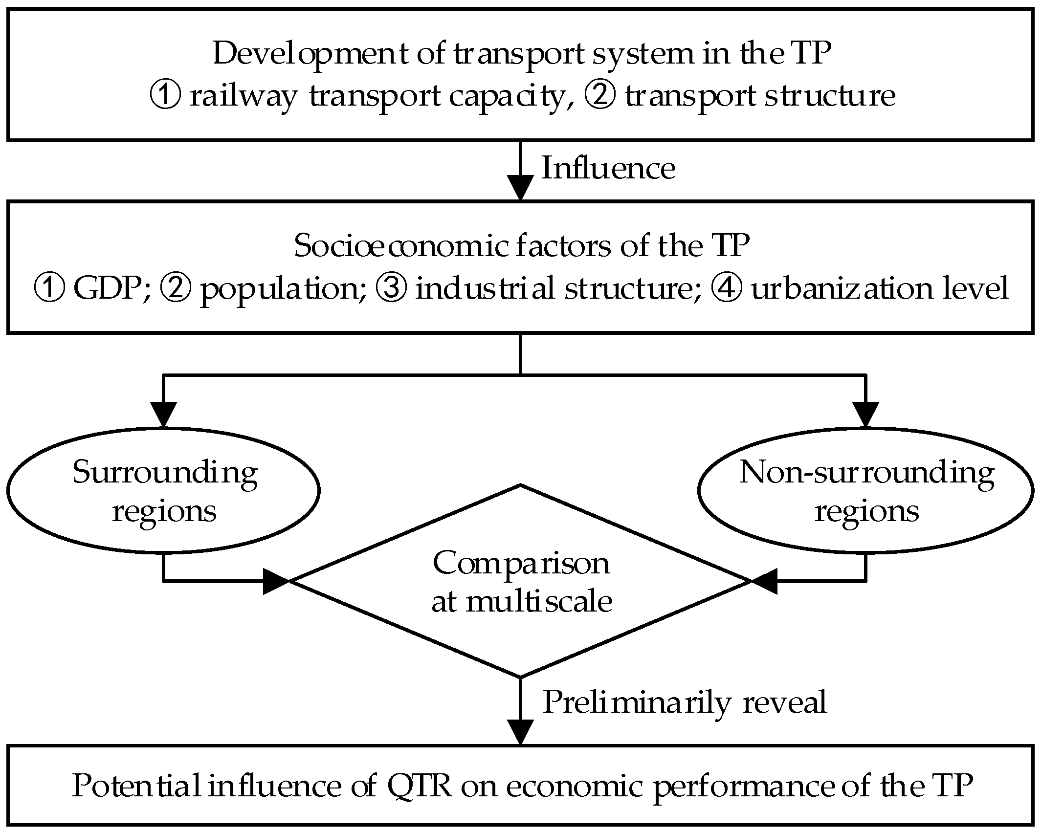
In this study, in order to reveal the potential influence of the QTR on the economic performance of the TP, the development of the transport system of the TP with the construction of the QTR was first studied. Then various socioeconomic factors were selected and their performance compared before and after the construction of the QTR, focusing on their differences between surrounding and non-surrounding areas. The results can be used to guide railway construction planning in the TP so as to promote sustainable socioeconomic development. It is our hope that the QTR will be seen as a good example of a sustainable railway that can be followed by other regions and countries.
2. Brief Introduction to the Qinghai–Tibet Railway
As the main region of the Third Pole, the TP has a very harsh natural environment [
26,
27]. Consequently, compared with the mid-east areas of China, transportation infrastructure here is lacking. Before 1955, freight could only be transported into Tibet by camel. For the period 1955–1978, a highway was available. In 1978, the construction of the QTR began with government support, and it is still considered a landmark project [
5,
15], despite raising serious concerns about its potential environmental impacts. As a result, the Chinese government has invested a large amount of money to protect the TP’s fragile ecosystem [
5].
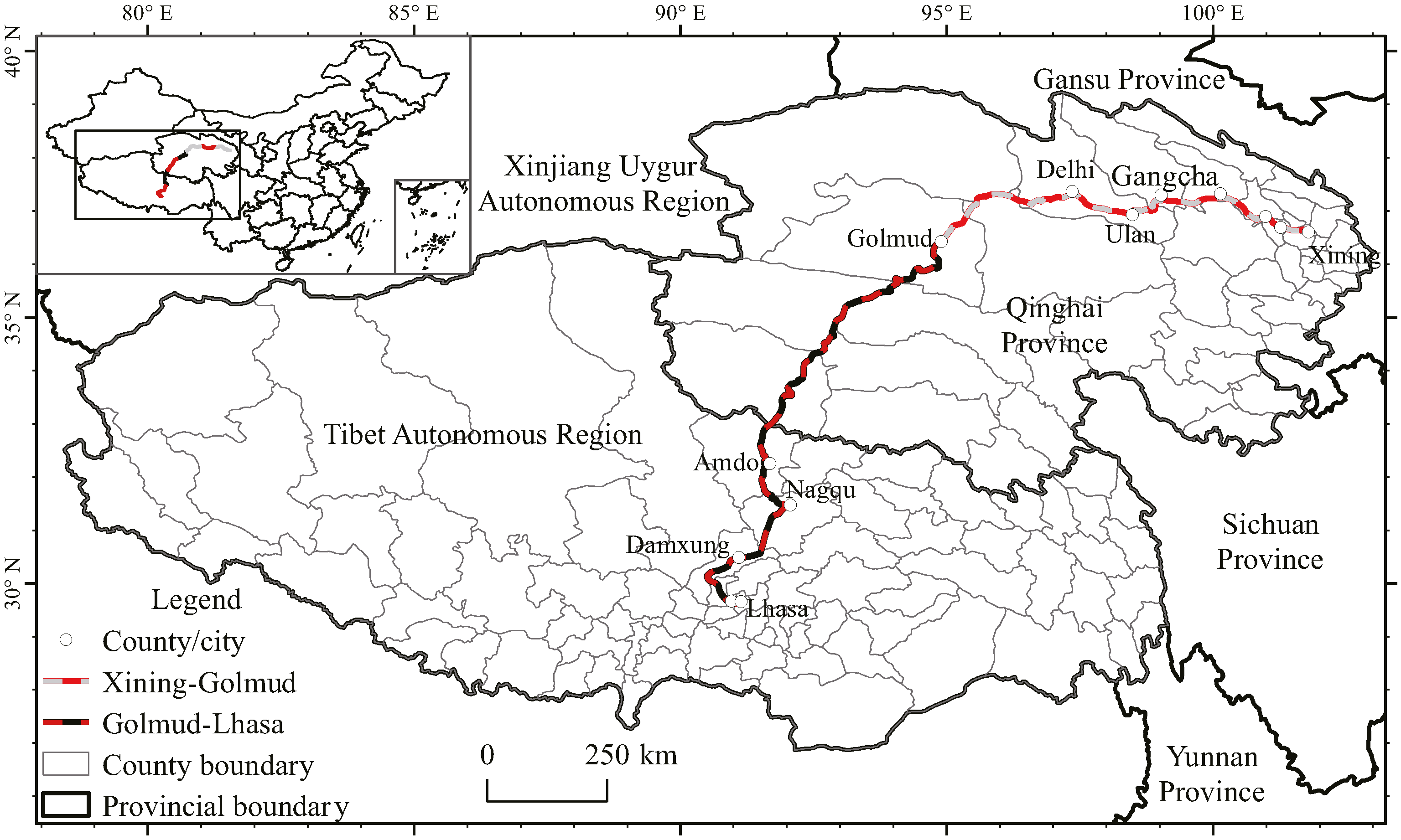
The QTR connects Xining, the capital of Qinghai Province, to Lhasa, the capital of the Tibet Autonomous Region. The first section of the QTR was opened to traffic in 1984, starting from Xining (XG) and ending at Golmud (GL) (
Figure 1), with a length of 814 km. The second section was inaugurated and opened to a regular trial service in July 2006, starting from GL and ending at Lhasa (
Figure 1), with a length of 1142 km. To minimize the negative influence of human activities on the environment of this area, 38 of the 45 stations in this section are unstaffed [
5]. The length of the entire line is 1956 km, 550 km of which were laid on permafrost [
28]. A network of tunnels was added to avoid disrupting the seasonal migration routes of animals [
5].
The important technical details of the QTR are as follows. The XG section is double track and the GL section is single track. The design speed for the QTR is 160 km/h, and the commercial speed for the XG section is 140 km/h (since 20 March 2015) and 120 km/h for the GL section. Note that the commercial speed for sections laid on permafrost is 100 km/h [
29]. Various measures were taken to ensure the stability of the railway embankment in permafrost regions [
29]. In terms of traction, at first, diesel-powered locomotives were used for the whole line, but electric locomotives have been used for the XG section since June 2011. The maximum train lengths for passenger trains and freight trains are 650 m and 850 m, respectively. The passenger carriages used on the QTR line are specially built and fully enclosed and have an oxygen supply for each passenger [
30]. Signs in the carriages are in Tibetan, Chinese, and English. The line has a capacity of eight pairs of passenger trains. Since October 2006, five pairs of passenger trains run on the GL section and one further pair on the XG section [
31].
4. Results
4.1. Evolution of the Transport System in the TP with the Construction of the QTR
First, the passenger traffic, freight traffic, passenger-kilometers, and freight-kilometers of the QTR for the period 1982–2013 are presented below. Then the passenger- and freight traffic-based transport structures of the TP for the period 1990–2013 are presented. Finally, the passenger-kilometers and freight-kilometers based transport structures of the TP for the period 1990–2013 are analyzed.
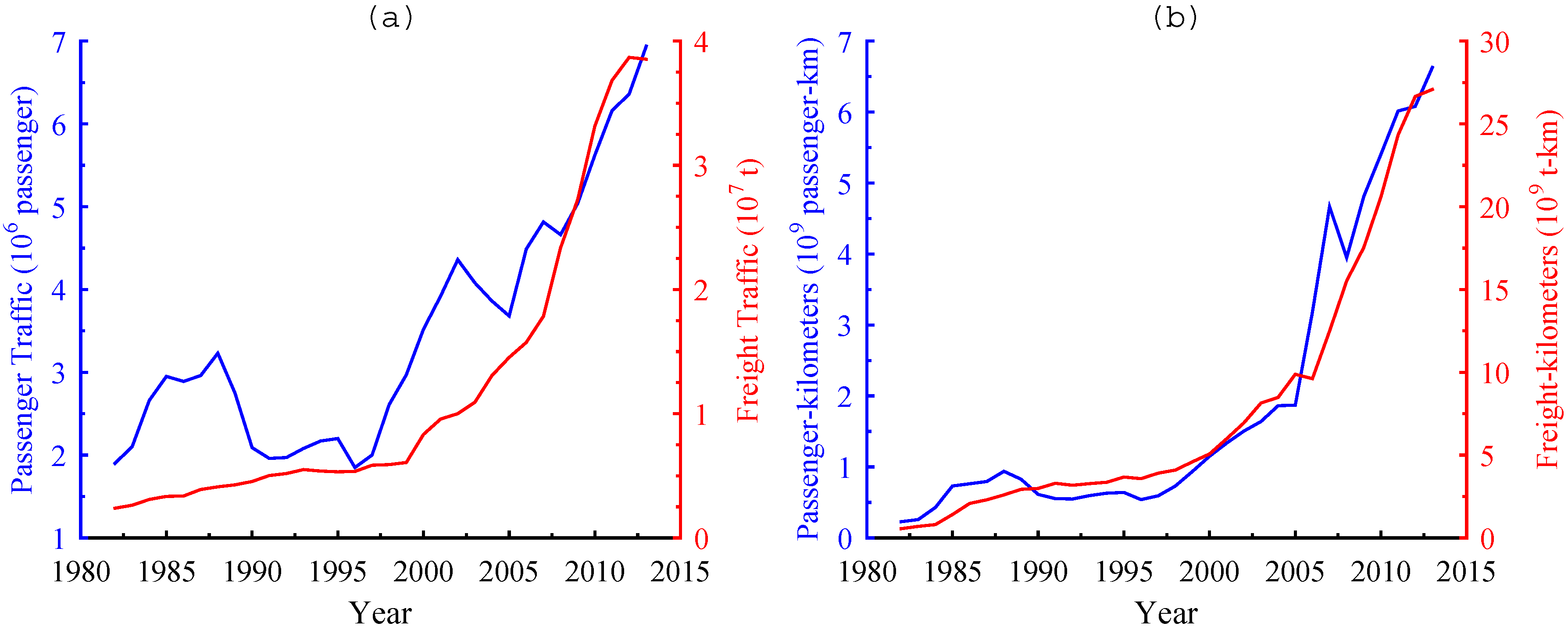
4.1.1. Analysis of Transport Capacity of the QTR for 1982–2013
On the whole, passenger traffic on the QTR increased for the period 1982–2013 (
Figure 3a). A marked increase can be seen after 1984, when the XG section opened to traffic, and after 2006, when the GL section opened. One thing to note in particular is the decrease in passenger volume in 2008 compared with previous years. This was due to civil unrest (the March 14 riot), which involved beatings, vandalism, looting of shops, and arson. Damage was estimated at more than 244 million Yuan (basic unit of currency in China) [
40].
Regarding freight traffic on the QTR in the period 1982–2013, a more rapid and steadily increasing tendency can be seen. During the 1980s and 1990s, freight traffic and its rate of increase were both low. In the 21st century, freight traffic presents a nearly exponential growth trend, which potentially can be explained by the construction of the GL section in 2001 and the completed line opening to traffic in 2006. In addition, more types of freight were transported to Tibet via the QTR. For example, petroleum products, including gas and diesel, which previously could only be transported to Tibet by highway and pipeline, were transported by railway for the first time on 5 May 2014 [
41]. This not only cut transportation costs but also made the transportation of petroleum products much safer.
Passenger-kilometers and freight-kilometers for 1982–2013 are presented in
Figure 3b. Compared with the highway, the railway is the major long-distance mode of transport. Therefore, compared with passenger and freight traffic values alone, the data for the passenger-kilometers and freight-kilometers of the QTR give a better insight into railway transport since they are the product of transport traffic and transport distance. From
Figure 3b, two phases for both passenger-kilometers and freight-kilometers can be identified: the slow increasing phase for 1982–2005 and the rapid, increasing phase for 2006–2013, which is potentially related to the opening of the GL section to traffic in 2006. In 1982, the passenger-kilometers and freight-kilometers were 0.2 × 10
9 passenger-km and 0.6 × 10
9 t-km, respectively, which increased to 1.9 × 10
9 passenger-km and 9.9 × 10
9 t-km, respectively, in 2005, increases of 1.7 × 10
9 passenger-km and 9.3 × 10
9 t-km, respectively. In 2013, the corresponding values were 6.6 × 10
9 passenger-km and 27.1 × 10
9 t-km, which increased by 4.7 × 10
9 passenger-km and 17.2 × 10
9 t-km respectively. The annual increases in passenger-kilometers and freight-kilometers for the second phase were 9.1 and 9.6 times those of the first phase, respectively.
4.1.2. Passenger and Freight Traffic-Based Transport Structure in the TP for 1990–2013
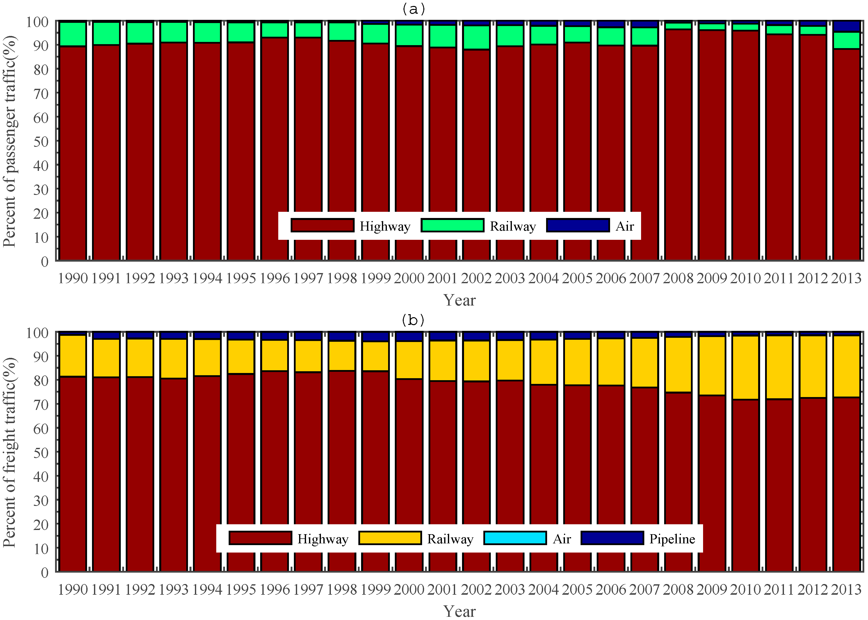
Figure 4 shows the passenger- and freight traffic-based transport structure of the TP. From
Figure 4a, it can be seen that highway passenger traffic maintained a dominant position in the TP for 1990–2013, and the average percentage of total traffic for that period was 91.31%. For railway passenger traffic, the percentage was low in each year and the average value was only 7.22%. The average ratios of highway, railway, and air passenger traffic were 91.31:7.22:1.48, respectively. Note that the significant decrease in the percentage of railway passenger traffic after 2008 was probably related to the outbreak of civil unrest mentioned above [
40].
Figure 4b shows the freight traffic-based transport structure of the TP. The average ratios of highway, railway, air, and pipeline freight traffic were 78.66:15.57:0.01:2.76, respectively, which indicated that highway freight traffic remained in a dominant position. For railway freight traffic, the percentage was low in each year and the average value was 15.57%, but it can be seen that the percentage increased in the period 2000–2013, which matches well with the time point of the GL section’s construction and opening to traffic. In 2000, the ratios of highway, railway, air, and pipeline freight traffic were 80.34:15.76:0.02:3.88, respectively, and in 2013 they were 72.65:25.86:0.02:1.47, respectively. The proportion of railway freight traffic increased by 10.10%.
4.1.3. Passenger- and Freight-Kilometers Based Transport Structures in the TP for 1990–2013
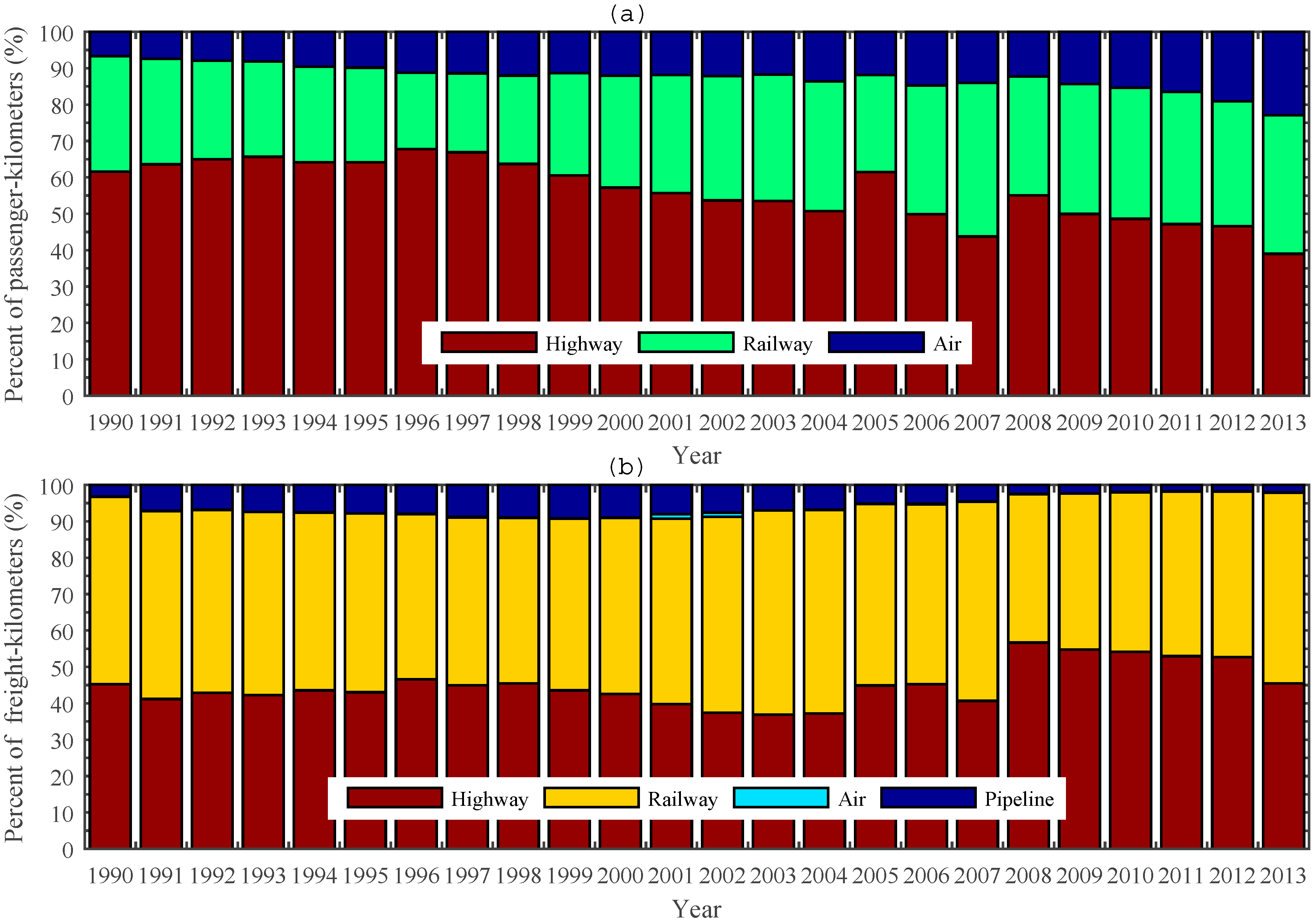
As mentioned above, the railway is more often used than the highway to transport passengers and freight over longer distances. Therefore, the passenger-kilometers and freight-kilometers based transport structures are also important aspects of the transport structure (
Figure 5).
From
Figure 5a it can be seen that the percentage of highway passenger-kilometers decreased gradually between 1990 and 2013 as a whole, from 61.56% in 1990 to 38.99% in 2013, and the percentage of air passenger-kilometers gradually increased, from 6.67% in 1990 to 22.96% in 2013. In terms of railway passenger-kilometers, first there was a decreasing trend for 1990–1996 followed by an increasing trend for 1996–2007. In 2007, one year after the QTR was fully opened to traffic, the percentage of railway passenger-kilometers reached 42.22%, which was the maximum for the whole study period. After that, a relatively stable period for 2008–2013 followed. The average ratios of highway, railway, and air passenger-kilometers were 56.46:31.10:12.44, respectively, for 1990–2013.
The freight-kilometers based transport structure of the TP is presented in
Figure 5b. It can be seen that both the railway and the highway maintain their dominant positions. The average ratios of highway, railway, air, and pipeline freight-kilometers were 45.00:48.99:0.15:5.86, respectively. Railway freight-kilometers were higher than highway freight-kilometers, not only the average value but also for 18 of the 24 time points between 1990 and 2013.
Taking the above analysis and the fact that the initial railway network of Tibet will be constructed and the length of the railway in Tibet will reach 1300 km by 2020 into account, we can predict that the highway-dominated transport system will break up and an integrated transport system will form in the TP. Since the QTR and the coming railway network are environmentally friendly, it can also be said that a more sustainable transport system will come to the TP.
4.2. Comparisons of GDP
GDP is usually used to describe the economic performance of a country or region. Based on the available data, the GDP at the county and 1 km scales for 2000, 2005, and 2010 were analyzed to reveal the economic performance of the surrounding and non-surrounding areas of the QTR before and following its opening.
In 2000, only the XG section was open to traffic. The comparison of GDP between 2000 and 2005 reflects the effects of the XG section on the economic performance of its surrounding areas. Similarly, the comparison between 2000/2005 and 2010 reflects the impacts of the entire line, especially the GL section, on the economy of its surrounding areas.
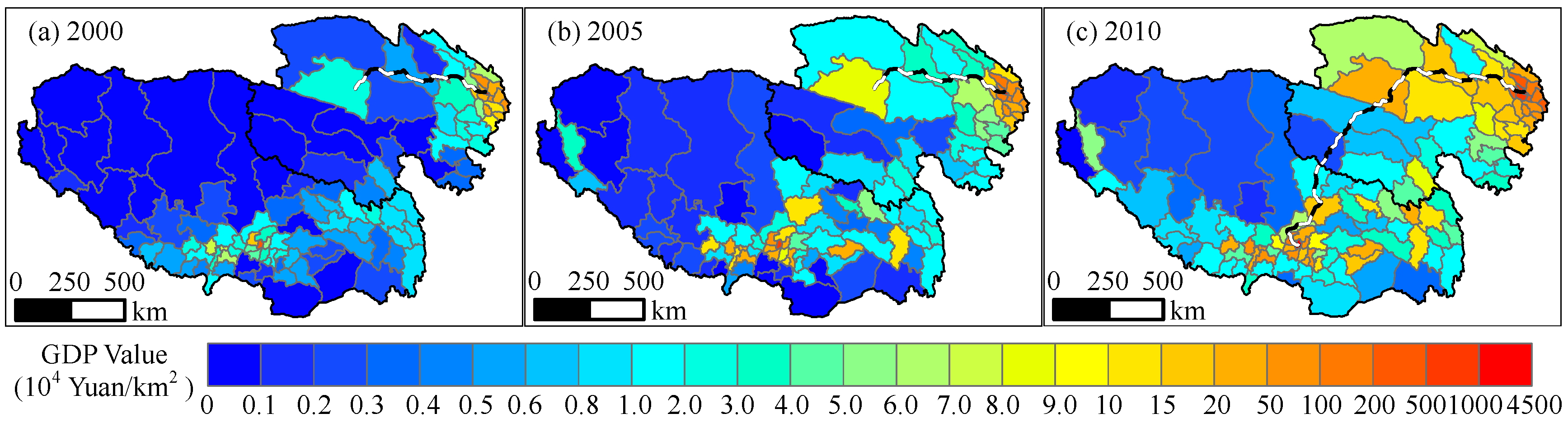
4.2.1. Comparisons at the County Scale
Figure 6 shows the GDP density values of the TP for 2000, 2005, and 2010. In terms of the spatial patterns of GDP density, the counties with high values were distributed mainly in the Yellow River–Huangshui River Valley in 2000. The GDP density of all counties surrounding the XG section increased over the period 2000–2005, especially in the Yellow River–Huangshui River Valley. At the same time, the GL section was under construction, and the GDP density of its surrounding areas also presented a slightly increasing trend. In 2010, the GDP density of the counties along the entire line increased markedly, especially along the GL section, compared with 2000 and 2005. However, as one of the least populated regions of China, the initial portion of the GL section (including Zhiduo, Qumalai, Anduo, and Nierong counties) saw a low rate of increase in GDP density. This is because two nature reserves, Kekexili (Hoh Xil) and Qinghai Sanjiangyuan, were established along this section [
5], and large-scale exploitation of nature reserves has been forbidden by the government as a measure to implement sustainable development.
For comparison, both the average GDP density and the AGR of GDP of surrounding and non-surrounding counties were calculated for 2000, 2005, and 2010 (
Table 1). The average GDP density of surrounding counties was greater than that of non-surrounding counties over three time points. In 2000, the GDP values for surrounding and non-surrounding counties were 2.71 yuan/km
2 and 0.88 yuan/km
2, respectively, a ratio of 3.1:1. By 2010, they had increased to 20.61 and 5.69 yuan/km
2, respectively, a ratio of 3.6:1.
The average GDP density showed an increasing tendency both for surrounding and non-surrounding counties for the period 2000–2010. However, the AGR values of surrounding counties were greater than those of non-surrounding counties for the periods 2000–2005, 2005–2010, and 2000–2010, which was probably related to the opening to traffic of the QTR (
Table 1). For instance, during the first ten months of its operation, trade between Tibet and external regions increased by 75%, to 2.6 billion yuan [
4].
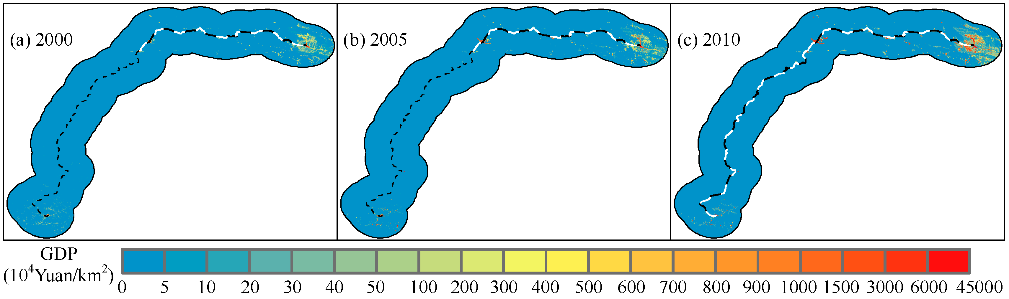
4.2.2. Comparisons at the 1 km Scale
Compared with the counties of the mid-east regions of China, the land areas of most counties of the TP are very large. The average area of counties in China is ~0.34 × 10⁴ km2, while the average area of counties in Qinghai and Tibet is ~1.69 × 10⁴ km2. Thus, the county-scale comparison is inadequate to reflect the details of GDP growth differences between surrounding and non-surrounding areas. Therefore, an analysis at the 1 km scale was carried out further.
In this study, of the QTR, ten buffer areas of the 1 km GDP dataset from 0 to 100 km with 10 km intervals (
Figure 7) were extracted. It can be seen that, except for Xining and Lhasa and their surrounding regions, the other buffer regions of the QTR had a lower GDP value for the three time points. From 2000 to 2005, the GDP value of Xining and its near areas increased markedly, while that of the other regions changed little. Between 2005 and 2010, the GDP values of Xining and Lhasa and their surrounding areas increased even more markedly.
For each buffer region centered on the QTR, the mean GDP and the AGR of GDP for the periods 2000–2005, 2005–2010, and 2000–2010 were calculated (
Table 2). It can be seen that GDP was high in the 0–10 km buffer region and lower in other buffer regions. In other words, GDP was concentrated mainly in the 0–10 km region in 2000, 2005, and 2010. Overall, the closer a region was to the railway, the greater the GDP value in each time period.
In terms of the AGR of GDP, except for that of the 90–100 km buffer region for 2000–2005, all other values were positive. In general, for all three time periods, the closer to the railway, the greater the AGR. The mean AGR values of all ten buffer regions for 2000–2005 and 2005–2010 were 17.95% and 22.39%, respectively, which meant that following the opening of the entire line to traffic, the GDP of the surrounding areas of the QTR had a greater growth rate than before the opening.
4.3. Comparisons of Population
The railway is capable of transporting people to its surrounding areas to engage in various socioeconomic activities [
42]. By analyzing changes in the population of these surrounding areas, the influences of the QTR on population distribution in the TP can be determined.
4.3.1. Comparisons at the County Scale
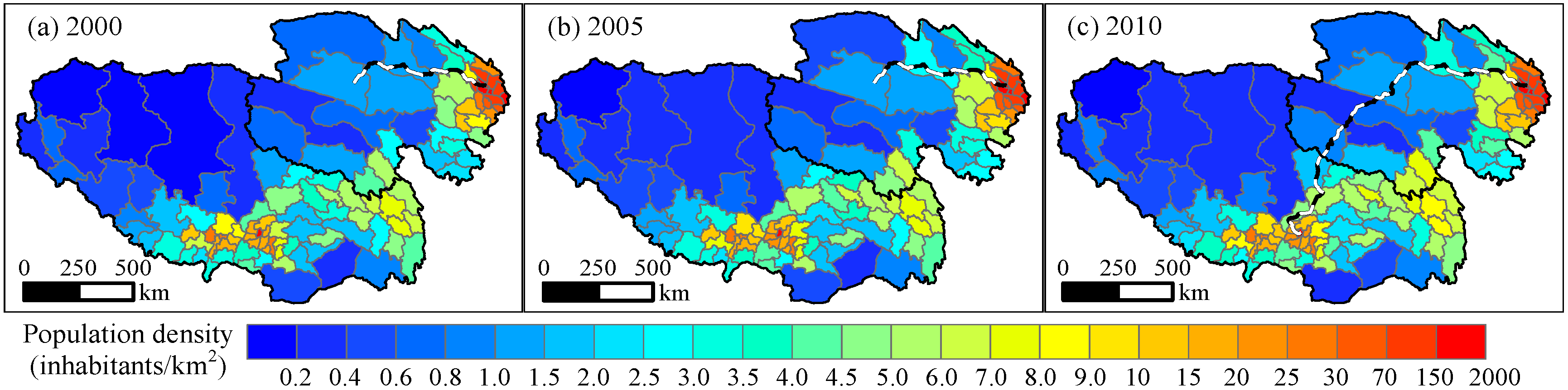
The population densities of both Qinghai and Tibet at the county scale for 2000, 2005, and 2010 are presented in
Figure 8. In 2000, the population was distributed mainly in the valley regions of the Yellow River–Huangshui River and their near regions and the valley regions of the Brahmaputra River and its tributaries. The population densities of other regions were lower than these values. For 2005 and 2010, a similar pattern of population density could be detected. In other words, between 2000 and 2010, the populations of both Qinghai and Tibet were not concentrated in the surrounding areas of the QTR.
For comparison, the mean population densities and the AGR of population of surrounding and non-surrounding counties were calculated for 2000, 2005, and 2010 (
Table 3). The mean population density of surrounding counties was greater than that of non-surrounding counties. For 2000, the corresponding values for surrounding and non-surrounding counties were 4.70 and 3.55 inhabitants/km
2, respectively, a ratio of 1.32:1. By 2010, these values had increased to 5.05 and 4.14 inhabitants/km
2, respectively, a ratio of 1.22:1.
The average population density showed an increasing tendency both for surrounding and non-surrounding counties for the period 2000–2010. However, the AGR of surrounding counties was lower than that of non-surrounding counties for the periods 2000–2005, 2005–2010, and 2000–2010. The biggest difference occurred for the period 2000–2005. The AGR of non-surrounding areas was 1.08%, while that for surrounding areas was only 0.05%. From a sustainability perspective, the fact that population grew more rapidly in non-surrounding counties than surrounding counties indicated that the QTR could be seen as a good example of sustainable transport.
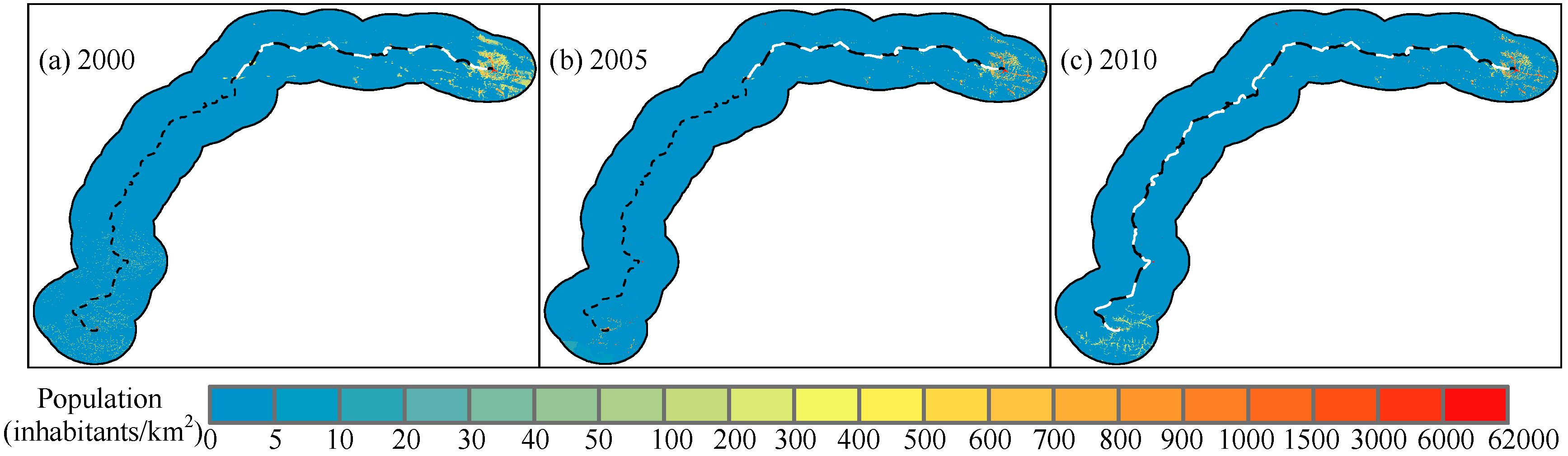
4.3.2. Comparisons at the 1 km Scale
Like GDP analyses at the 1 km scale, the population comparison at the county scale is inadequate to reflect the details of differences in population changes between surrounding and non-surrounding areas. Therefore, further comparisons at the 1 km scale were carried out.
In this study, of the QTR, ten buffer areas of the 1 km population dataset from 0 to 100 km with 10 km intervals were extracted (
Figure 9). It can be seen that the surrounding areas of the QTR were sparsely populated and the population was concentrated mainly in Xining and Lhasa and their surrounding areas. In terms of changes in the spatial distribution of population, no obvious changes could be detected for the period 2000–2010.
In addition, statistical analysis was carried out for the ten buffer areas centered on the QTR (
Table 4). This shows that for 2000, 2005, and 2010, population density was high for the 0–10 km buffer region and lower for other buffer regions. That is to say, the population was concentrated mainly in the 0–10 km buffer region.
In terms of the AGR of population between 2000 and 2005, various fluctuations could be detected and no regular patterns could be found for any of the buffer regions. For the period 2005–2010, all buffer regions had positive AGR values that were more stable than those for the period 2000–2005. The changes in AGR for 2000–2010 were similar to those of 2000–2005 and 2005–2010.
The above analyses indicated that population was not concentrated in surrounding areas of the QTR for the period 2000–2010 whether at the county scale or the 1 km scale. As an environmentally and culturally sensitive area, the TP’s low population density is actually favorable to sustainable development. In addition, one possible reason for this is the sustainable development policies implemented here, including Kekexili (Hoh Xil) and Qinghai Sanjiangyuan nature reserves [
5] and unstaffed railway stations. Another possible reason is that the operating period of the railway appears to have not been long enough to generate substantial changes in population distribution.
4.4. Comparisons of Industrial Structure
Industrial structure is the basis and core of economic structure, and it can be influenced by railway transportation [
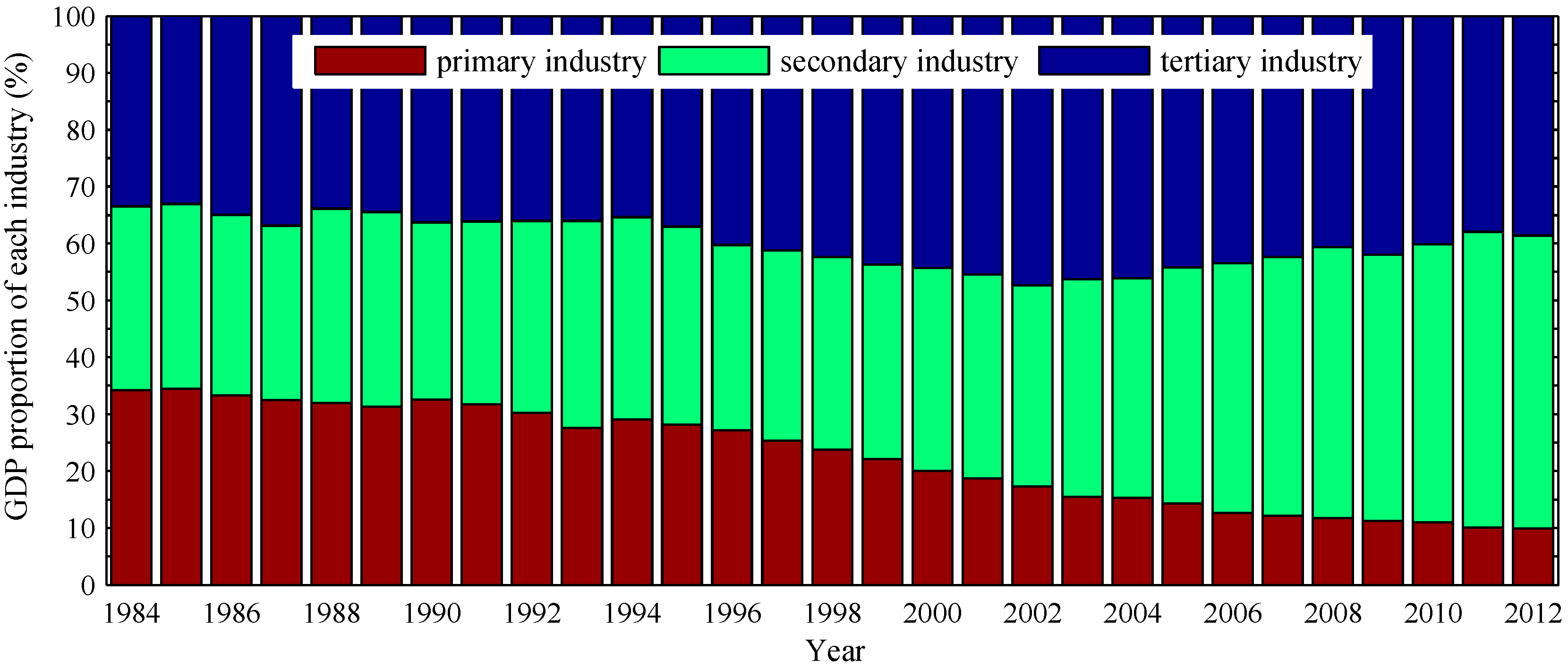
43]. The industrial structure of Qinghai–Tibet is illustrated in
Figure 10.
The production values of primary industry (PI), secondary industry (SI), and tertiary industry (TI) had been increasing for both Qinghai and Tibet between 1984 and 2012 [
31,
32], but in terms of industrial structure, the proportion of PI decreased continuously in the same period, while the proportion of SI and TI increased overall (
Figure 10). In 1984, the ratios of PI, SI, and TI were 34.2:32.3:33.5. For 2012, the ratios were 9.9:51.5:38.6, and the combined percentage of SI and TI exceeded 90%.
In terms of the different stages of construction, for 1984–2001 when construction of the GL section had not begun, the percentage of PI decreased continuously, that of TI increased continuously, and that of SI remained fairly stable. For 2002, the ratios of the three industry types were 17.3:35.3:47.4. Compared with that in 1980, the percentage of TI increased by 21.68%. Since the GL section opened to traffic in 2006, the percentage of PI decreased continuously, that of TI remained fairly stable, while that of SI increased markedly, and it increased by 16.02% in the period 2002–2012. The above results indicate that the opening of the QTR probably helped to optimize the industrial structure of the TP, which is consistent with the conclusion drawn by Wu [
44]. In addition, as an important component of TI, tourism boomed on the plateau ten years after the opening of the QTR to traffic [
45].
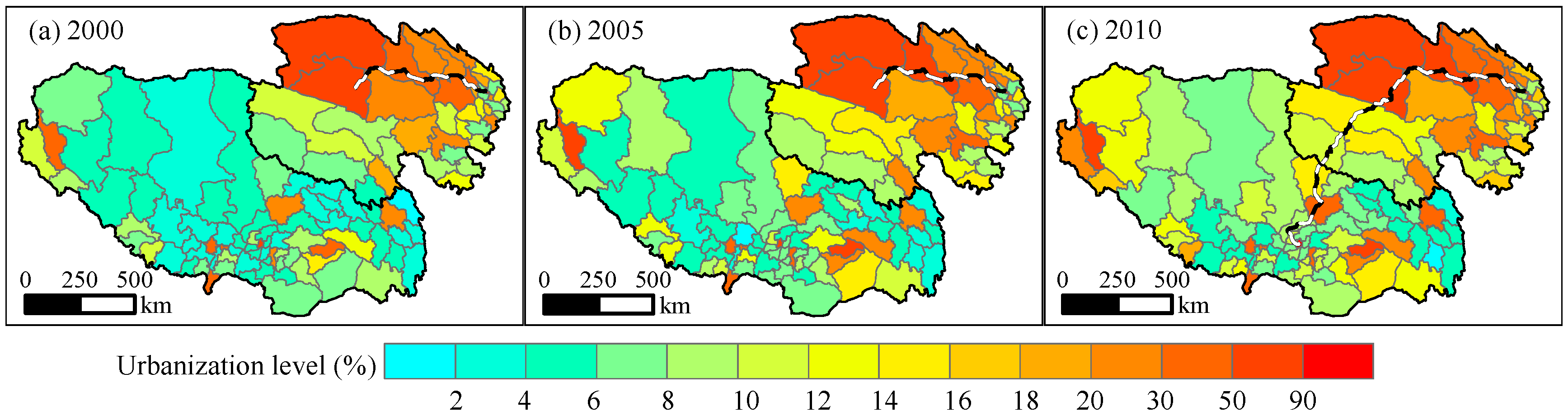
4.5. Comparisons of the Urbanization Level
Urbanization level (UL), and its changing trends, are important components of socioeconomic activity, and it refers to the proportion of non-agricultural population to total population. Changes in UL can reflect the process of migration of population to cities and urban areas. Non-agricultural population refers to those people engaged in SI and TI and the people they support.
Figure 11 illustrates the UL of both Qinghai and Tibet at the county scale. Those counties surrounding the XG section of the QTR had a relatively high UL, whereas most other counties had a low UL for 2000, 2005, and 2010. In terms of changes in the spatial distribution of the UL, an increase can be seen in the surrounding counties of the QTR.
For comparison, the average UL values of surrounding and non-surrounding areas of the QTR for 2000, 2005, and 2010 were calculated (
Table 5). It can be seen that the UL values of surrounding areas were greater than those of non-surrounding areas for the three time points. The average UL value of surrounding areas of the QTR for 2000, 2005, and 2010 was 47.06%, and that for non-surrounding areas was 12.63%, a ratio of 3.73:1. The UL of surrounding and non-surrounding areas increased gradually over the period 2000–2010, but the AGR of non-surrounding areas was greater than that of surrounding areas in the periods 2000–2005, 2005–2010, and 2000–2010, which means that the QTR had no obvious impact on changes in the UL of its surrounding areas in those time periods.
5. Discussion
In this study, the evolution of the transport system in the TP following the construction of the QTR was analyzed, followed by a comparison of four factors between surrounding and non-surrounding areas before and after construction, and finally the changes in these factors under the influence of the QTR were examined. However, some uncertainties still exist.
First, it should be noted that data related to the QTR are difficult to acquire since both Qinghai and Tibet are remote regions and record keeping for these regions lags behind other regions of mid-east China. For example, because of a lack of GDP and population data at the town scale, they could only be analyzed at the county scale. However, the land areas of counties in both Qinghai and Tibet are very large. Some of them are even greater in size than provinces in mid-east China. Therefore, comparison at the county scale is inadequate to reflect the details of the influence of the QTR on economic performance. Although the 1 km GDP and population datasets were analyzed further, the uncertainties in these datasets might have extended to the results of this study since they were produced based on an algorithm devised for the national scale [
38,
39].
Second, changes in infrastructures and economic conditions in Tibet have attracted a large proportion of the floating population since the 1990s [
46]. Some studies show that the floating population is becoming the major power for accelerating urbanization in modern times, and it is estimated that temporary residents may account for about half of the urban population in Tibet [
47]. However, the population data obtained for this study did not contain the floating population, so the population density, the AGR of population, and the UL of the surrounding areas may therefore be underestimated. Other evidence also shows that Tibet has seen a surge of Han migrants, which has been further boosted by the QTR [
4,
48]. Once data with high precision and resolution become available, more objective conclusions can be drawn in future studies.
Our results indicate that the influences of the QTR on the GDP of its surrounding areas are obvious, which is consistent with the results of Wang and Wu [
25]. However, the influences of the QTR on population and UL of its surrounding areas are not so obvious. Some possible reasons are listed below. In fact, compared with the Qinghai–Tibet Highway, which had operated for 60 years, the traffic extension of the QTR was not so obvious (
Figure 4 and
Figure 5). In addition, because the TP is a unique and fragile high-altitude ecosystem, the QTR construction project has raised serious concerns about its possible environmental consequences [
15]. As a result, the Chinese government and local officials developed a green and sustainable policy that emphasized protection of soils, vegetation, animals, and water resources. In addition, five nature reserves along the route were established [
4,
5]. In other words, the construction of the QTR has been achieved with ecological protection at the top of the project’s agenda, which will certainly restrict the economic development of its surrounding areas. Moreover, the QTR is a young railway, and only ten years have passed since the entire line opened to traffic in 2006. Moreover, the construction of the supporting infrastructure of the QTR is incomplete and not comprehensive. Finally, compared with railways located in the mid-east region of China, the natural environmental conditions surrounding the QTR are very harsh and 965 km of the line runs at an altitude greater than 4000 m [
49]. Therefore, it will take considerably more time for the QTR to influence the socioeconomic development of its surrounding areas.
This comparison work is only an initial study into the influence of the QTR on the economic performance of the TP. In fact, as well as the QTR’s influence, the development of the region is tied to other factors, including financial support from central government [
50]. Therefore, on the basis of this study, future analyses of the changes in accessibility to and economic linkages of the TP with surrounding regions will be more significant and overcome these uncertainties.
With the passage of time, the transportation system and corresponding infrastructure of the TP are developing rapidly. For example, the Ministry of Transport of the People’s Republic of China has drawn up policies that the initial railway network of Tibet will be constructed and the length of the railway in Tibet will reach 1300 km by 2020 [
51]. Recently, the construction of the Lhasa–Xigazê Railway was completed in July 2014 and was formally opened a month later [
52]. As an extension of the QTR, designed with a capacity of more than 8.3 million tons of freight per annum, it will promote the economic development of Xigazê, as well as Tibet, by reducing transportation costs and promoting tourism. In addition, the Lanzhou–Xinjiang High-Speed Railway in northwestern China, from Lanzhou in Gansu Province to Ürümqi in the Xinjiang Uyghur Autonomous Region, was opened in December 2014 [
53]. It is routed from Lanzhou to Xining before heading northwest into the Hexi Corridor at Zhangye, which makes it the first high-speed railway to go through the TP. In other words, a railway network will exist here in the near future. When the railway network era of the TP finally arrives, Tibet, Qinghai, Xinjiang, Gansu, Sichuan, and Yunnan provinces will be more closely connected by railway, which means that more relevant studies can be carried out. For example, the construction and development of the railway network in the TP is potentially beneficial to the Belt and Road Initiative—where “Belt” refers to the Silk Road Economic Belt and ”Road” refers to the 21st Century Maritime Silk Road [
54].
The railway network will boost the socioeconomic development of this region by moving people into it [
5,
46]. However, it must be mentioned that, from a sustainability perspective, the QTR and the coming railway network will need to be carefully managed to promote and ensure long-term ecosystem health and sustainability in western China. Only then can sustainable railway networks be followed in other regions.


