
Spatial and Temporal Evolution of Urban Systems in China during Rapid Urbanization


Abstract
:1. Introduction
2. Literature Review
2.1. City Size Distribution and Chinese Cities
2.2. The Underlying Forces for Urban Hierarchical Formation
3. Data and Methodology
3.1. Data and Indicators
3.2. Methods and Models
3.2.1. Estimate of the Pareto Exponent
3.2.2. Non-Radial Directed Distance Function
3.2.3. Sequential Malmquist TFP Index
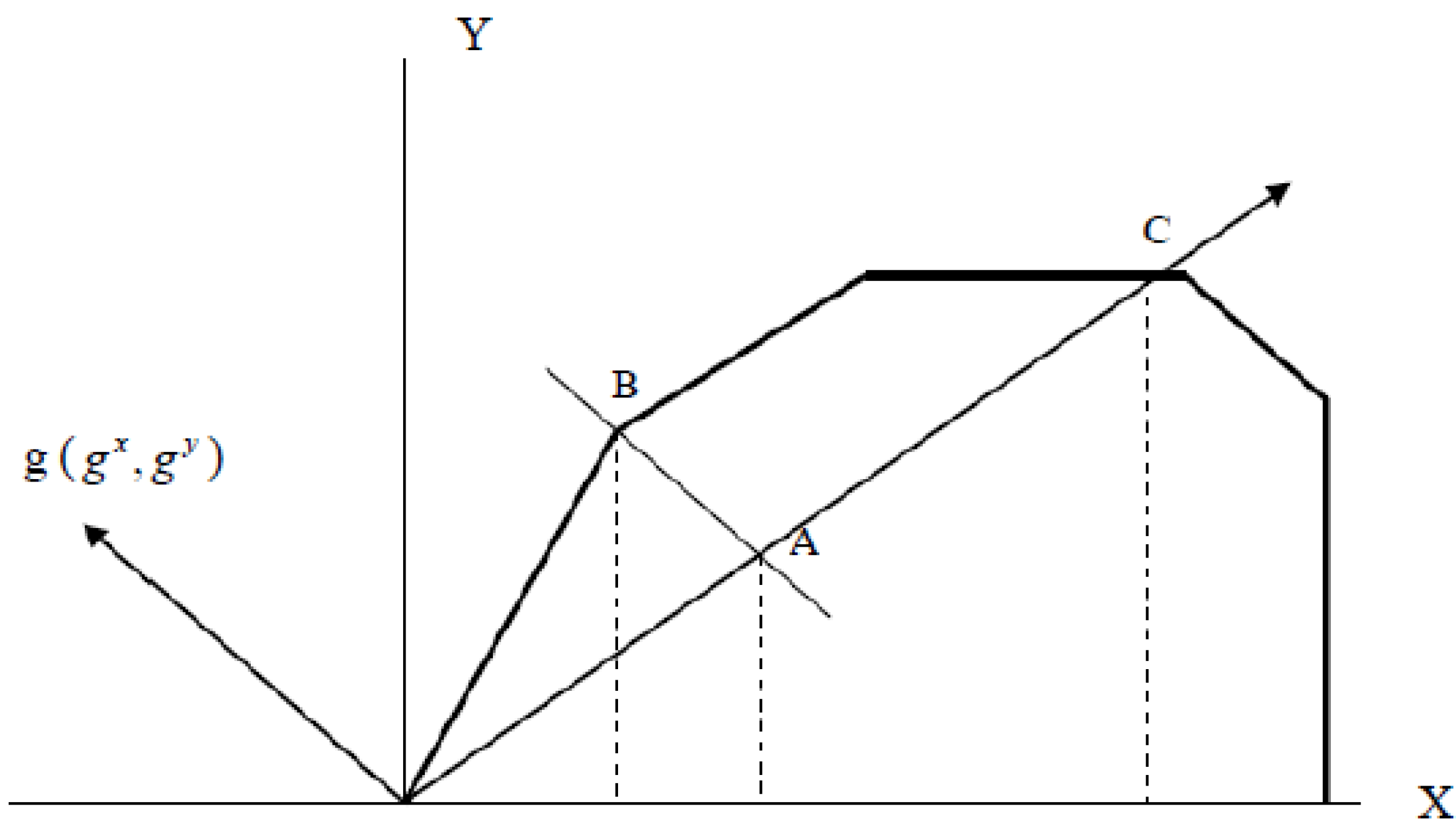
3.2.4. Projected Value Function
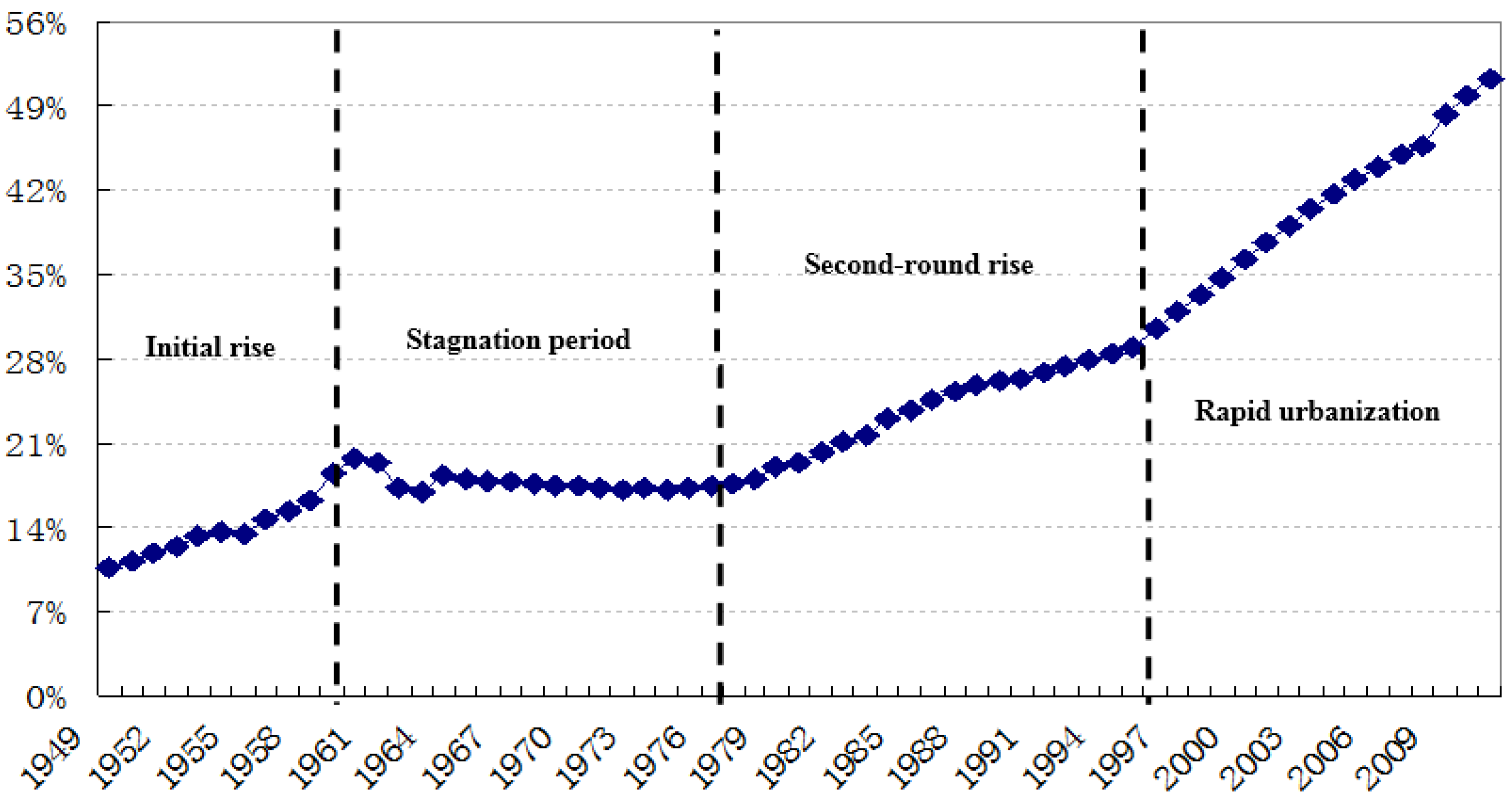
4. Urbanization and Urban Systems in China
5. Spatial-Temporal Evolution of Urban Systems
5.1. Spatial-Temporal Evolution of Cities
5.2. Empirical Test on Zipf’s Law and Gibrat’s Law
5.2.1. Empirical Test on Zipf’s Law
5.2.2. Empirical Test on Gibrat’s Law
6. Urban Hierarchy and Economic Efficiency
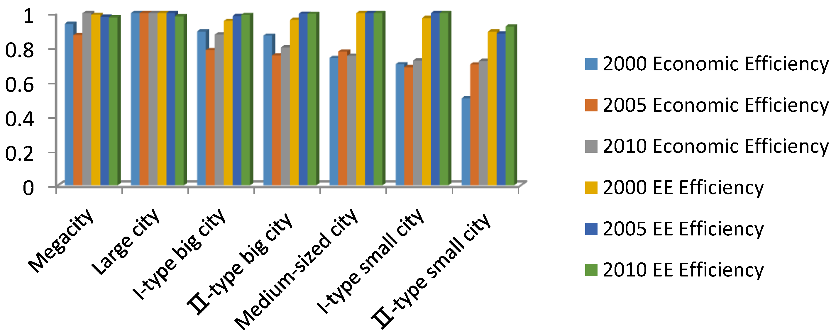
6.1. Comparison of Economic Efficiency and Economic-Environmental Efficiency
6.2. Total-Factor Efficiency Change and Decomposition
6.3. Input Savings Potential
7. Conclusions
Acknowledgments
Author Contributions
Conflicts of Interest
References and Notes
- Bigotte, J.; Antunes, A.; Krass, D.; Berman, O. The relationship between population dynamics and urban hierarchy: Evidence from Portugal. Int. Reg. Sci. Rev. 2014, 2, 149–171. [Google Scholar] [CrossRef]
- Maliszewski, P.; ÓhUallacháin, B. Hierarchy and concentration in the American urban system of technological advance. Pap. Reg. Sci. 2012, 4, 743–758. [Google Scholar] [CrossRef]
- Dimou, M.; Schaffar, A. Urban hierarchies and city growth in the Balkans. Urban Stud. 2009, 13, 2891–2906. [Google Scholar] [CrossRef]
- Wei, Y.H. State policy and urban systems: The case of China. J. Chin. Geogr. 1997, 7, 1–10. [Google Scholar]
- Bai, X.; Shi, P.; Liu, Y. Realizing China’s urban dream. Nature 2014, 509, 158–160. [Google Scholar] [PubMed]
- Henderson, J.V. Urbanization in China: Policy Issues and Options. Urban Stud. 2007, 4, 32–41. [Google Scholar]
- Chang, K.C.; Wen, M.; Wang, G.X. Social capital and work among rural-to-urban migrants in China. Asian Popul. Stud. 2011, 7, 275–292. [Google Scholar] [CrossRef]
- Sun, M.J.; Fan, C.C. China’s permanent and temporary migrants: Differentials and changes, 1990–2000. Prof. Geogr. 2013, 63, 92–112. [Google Scholar] [CrossRef]
- Cai, Y. China’s new demographic reality: Learning from the 2010 census. Popul. Dev. Rev. 2013, 39, 371–396. [Google Scholar] [CrossRef] [PubMed]
- Hopke, P.; Cohen, D.; Begum, B.; Biswas, S.; Ni, B.; Pandit, G.; Santoso, M.; Chung, Y.; Davy, P.; Markwitz, A. Urban air quality in the Asian region. Sci. Total Environ. 2008, 404, 103–112. [Google Scholar] [CrossRef] [PubMed]
- Matus, K.; Nam, K.-M.; Selin, N.E.; Lamsal, L.N.; Reilly, J.M.; Paltsev, S. Health damages from air pollution in China. Glob. Environ. Chang. 2012, 22, 55–66. [Google Scholar] [CrossRef]
- The Communist Party of China’s Committee. The 10th, 11th and 12th Five-year Plans for National Economic and Social Development (2001–2005, 2006–2010, 2011–2015). 2001, 2006, 2011. [Google Scholar]
- Li, Q.; Chen, Y.; Liu, J. The research on urbanization path of China. Soc. Sci. China 2012, 7, 82–100. [Google Scholar]
- Lim, E.; Spence, M. Medium and Long Term Development and Transformation of the Chinese Economy; China CITIC Press: Beijing, China, 2011. (In Chinese) [Google Scholar]
- Berry, B. City size distributions and economic development. Econ. Dev. Cult. Chang. 1961, 9, 573–588. [Google Scholar]
- Zipf, G. Human Behavior and the Principle of Least Effort; Hafner Publishing Company: New York, NY, USA, 1949. [Google Scholar]
- Henderson, J.V. The sizes and types of cities. Am. Econ. Rev. 1974, 4, 640–656. [Google Scholar]
- Rossi-Hansberg, E.; Wright, M. Urban structure and growth. Rev. Econ. Stud. 2007, 74, 597–624. [Google Scholar] [CrossRef]
- Gibrat, R. Les Inégalités Économiques; Sirey Publishers: Paris, France, 1931. (In French) [Google Scholar]
- Eeckhou, J. Gibrat’s law for (all) cities. Am. Econ. Rev. 2004, 5, 1429–1451. [Google Scholar] [CrossRef]
- Ye, X.Y.; Xie, Y.C. Re-examination of Zipf’s Law and urban dynamic in China: A regional approach. Ann. Reg. Sci. 2012, 1, 135–156. [Google Scholar] [CrossRef]
- Rosen, K.; Resnick, M. The size distribution of cities: An examination of the Pareto law and primacy. J. Urban Econ. 1980, 8, 165–186. [Google Scholar] [CrossRef]
- Gabaix, X. Zipf’s Law for cities: An explanation. Q. J. Econ. 1990, 3, 739–767. [Google Scholar] [CrossRef]
- Batty, M. Polynucleated urban landscapes. Urban Stud. 2001, 4, 635–655. [Google Scholar] [CrossRef]
- Soo, K.T. Zipf’s Law for cities. Reg. Sci. Urban Econ. 2005, 3, 239–263. [Google Scholar] [CrossRef]
- Duranton, G. Urban evolutions. Am. Econ. Rev. 2007, 1, 197–221. [Google Scholar] [CrossRef]
- Bettencourt, L. The origins of scaling in cities. Science 2013, 340, 1438–1441. [Google Scholar] [CrossRef] [PubMed]
- Levy, M. Gibrat’s Law for (all) cities: Comment. Am. Econ. Rev. 2009, 4, 1672–1675. [Google Scholar] [CrossRef]
- Bee, M.; Riccaboni, M.; Schiavo, S. The size distribution of US cities: Not Pareto, even in the tail. Econ Lett. 2013, 2, 232–237. [Google Scholar] [CrossRef]
- Wang, X.L.; Xia, X.L. Optimization of city scale for economic growth. Econ. Res. J. 1999, 9, 22–29. [Google Scholar]
- Au, C.; Henderson, J.V. Are Chinese cities too small? Rev. Econ. Stud. 2006, 3, 549–576. [Google Scholar] [CrossRef]
- Xu, Z.; Zhu, N. City size distribution in China? Urban Stud. 2009, 10, 2159–2185. [Google Scholar]
- Wang, X. Urbanization path and city scale in China. Econ. Res. J. 2010, 10, 20–32. [Google Scholar]
- Liang, Q.; Chen, Q.; Wang, R. Household register reform, labor flow and city system optimization. Soc. Sci. China 2013, 12, 36–60. [Google Scholar]
- National Bureau of Statistics of China (NBSC). China City Statistical Yearbook; China Statistic Press: Beijing, China, 1997–2014. (In Chinese)
- The State Council of China. The Adjustment of the Standard of City Type Classification; The State Council of China: Beijing, China, 2014. (In Chinese)
- Tan, R.; Wang, R.; Sedlin, T. Land-development offset policies in the quest for sustainability: What can China learn from Germany? Sustainability 2014, 6, 3400–3430. [Google Scholar] [CrossRef]
- Jin, X. Total-factor efficiency analysis of cities in China: 1990–2003. Shanghai J. Econ. 2006, 7, 14–23. [Google Scholar]
- Li, X.; Xu, X.; Chen, H. Temporal and spatial changes of urban efficiency in the 1990s. Acta Geogr. 2005, 4, 615–625. [Google Scholar]
- Gao, W. The comparable analysis of metropolitan productivity in China. Shanghai J. Econ. 2008, 7, 3–10. [Google Scholar]
- Guo, T.; Xu, Y.; Wang, Z. The analyses of metropolitan efficiencies and their changes in China based on DEA and Malmquist index models. Acta Geogr. 2009, 4, 408–416. [Google Scholar]
- Fang, C.; Guan, X. Comprehensive measurement and spatial distinction of input-output efficiency of urban agglomerations in China. Acta Geogr. 2011, 8, 1011–1022. [Google Scholar]
- Zhang, H.; Uwasu, M.; Hara, K.; Yabar, H. Sustainable urban development and land use change—A case study of the Yangtze River Delta in China. Sustainability 2011, 3, 1074–1089. [Google Scholar] [CrossRef]
- National Bureau of Statistics of China. The Sixth Census of Total Population in China; China Statistic Press: Beijing, China, 2011.
- Cooper, W.; Li, S.; Seiford, M.; Tone, K.; Thrall, M.; Zhu, J. Sensitivity and stability analysis in DEA. J. Product. Anal. 2001, 15, 217–246. [Google Scholar] [CrossRef]
- Liu, Y.Q.; Xu, J.P.; Luo, H.W. An integrated approach to modelling the economy-society-ecology system in urbanization process. Sustainability 2014, 6, 1946–1972. [Google Scholar] [CrossRef]
- Li, H.; Wei, Y.D.; Liao, F.H.; Huang, Z.J. Administrative hierarchy and urban land expansion in transitional China. Appl. Geogr. 2015, 56, 177–186. [Google Scholar] [CrossRef]
- Wang, K.; Wei, Y.; Zhang, X. Energy and emissions efficiency patterns of Chinese regions. Appl. Energy 2013, 104, 105–116. [Google Scholar] [CrossRef]
- Fukuyama, H.; Weber, W.L. A directional slacks-Based measure of technical inefficiency. Socio Econ. Plan. Sci. 2009, 43, 274–287. [Google Scholar] [CrossRef]
- Caves, D.; Christensen, L.; Diewert, W. Multilateral comparisons of output, input and productivity using superlative index numbers. Econ. J. 1982, 92, 73–86. [Google Scholar] [CrossRef]
- National Bureau of Statistics of China. The Fifth Census of Total Population in China; China Statistic Press: Beijing, China, 2001. (In Chinese)
- Tan, M.; Li, X.; Lu, C. Urban land expansion and arable land loss of the major cities in China in the 1990s. Sci. China 2005, 48, 1492–1500. [Google Scholar] [CrossRef]
- Sicular, T.; Yue, X.; Gustafsson, B.; Li, S. The urban-rural income gap and inequality in China. Rev. Income Wealth 2007, 53, 93–126. [Google Scholar] [CrossRef]
- Boyd, A.; Tolley, G.; Pang, J. Plant level productivity, efficiency, and environmental performance of the container glass industry. Environ. Resour. Econ. 2002, 1, 29–43. [Google Scholar] [CrossRef]
- Glaeser, E. Triumph of the City; Penguin Press: New York, NY, USA, 2011. [Google Scholar]
- Liu, Y.B.; Yao, C.S.; Wang, G.X.; Bao, S.M. An integrated sustainable development approach to modeling the eco-environmental effects from urbanization. Ecol. Indic. 2011, 11, 1599–1608. [Google Scholar] [CrossRef]
- Gong, Z.; Zhao, Y.; Ge, X. Efficiency assessment of the energy consumption and economic indicators in Beijing under the influence of short-term climatic factors. Nat. Hazards 2014, 71, 1145–1157. [Google Scholar] [CrossRef]
- Charnes, A.; Cooper, W.; Lewin, Y.; Seiford, M. Data Envelopment Analysis; Kluwer Academic Publishers: Dordrecht, The Netherlands, 1995. [Google Scholar]
- Wei, Y. Restructuring for growth in urban China: Transitional institutions, urban development, and spatial transformation. Habitat Int. 2012, 36, 396–405. [Google Scholar] [CrossRef]
- Ding, C.; Zhao, X. Assessment of urban spatial-Growth patterns in China during rapid urbanization. China Econ. 2011, 44, 46–71. [Google Scholar] [CrossRef]
- Anderson, G.; Ge, Y. The size distribution of Chinese cities. Reg. Sci. Urban Econ. 2005, 35, 756–776. [Google Scholar] [CrossRef]
- Zeng, C.; He, S.W.; Cui, J.X. A multi-level and multi-dimensional measuring on urban sprawl: A case study in Wuhan metropolitan area, central China. Sustainability 2014, 6, 3571–3598. [Google Scholar] [CrossRef]
- Glaeser, E. The challenge of urban policy. J. Policy Anal. Manag. 2012, 31, 111–122. [Google Scholar] [CrossRef]
- Xie, H.; Zou, J.; Jiang, H.; Zhang, N.; Choi, Y. Spatiotemporal pattern and driving forces of arable land-use intensity in China. Sustainability 2014, 6, 3504–3520. [Google Scholar] [CrossRef]
- Song, S.; Zhang, K. Urbanization and city-size distribution in China. Urban Stud. 2002, 39, 2317–2327. [Google Scholar] [CrossRef]
- Tan, R.; Qu, F. The path of farmland conversion in China: Governing reform replaces property reform. Manag. World 2010, 6, 56–64. [Google Scholar]


| Variables | Category | Indicator |
|---|---|---|
| Input | Capital | Investment in fixed assets for urban construction |
| Labor | Persons employed in districts of cities | |
| Land | Area of land used for urban construction | |
| Output | Expected Output | Gross domestic product |
| Unexpected Output | Pollution discharge |
| Size of Cities | 2000 | 2010 | Change Degree | |||
|---|---|---|---|---|---|---|
| Number of Cities | Population Proportion | Number of Cities | Population Proportion | Number of Cities | Population Proportion | |
| Megacity (Size ≥ 10,000,000) | 3 | 6.7 | 6 | 11.2 | 3 (+) | 4.5 |
| Large City (5,000,000 ≤ Size < 10,000,000) | 7 | 8.6 | 15 | 12.9 | 8 (+) | 4.3 |
| Type I Big City (3,000,000 ≤ Size < 5,000,000) | 19 | 13.3 | 29 | 15.2 | 10 (+) | 1.9 |
| Type II Big City (1,000,000 ≤ Size < 3,000,000) | 135 | 40.4 | 167 | 39.9 | 32 (+) | −0.5 |
| Medium-sized City (500,000 ≤ Size < 1,000,000) | 92 | 13.3 | 94 | 9.1 | 2 (+) | −4.2 |
| Type I Small City (200,000 ≤ Size < 500,000) | 212 | 12.5 | 229 | 9.6 | 17 (+) | −2.9 |
| Type II Small City (Size < 200,000) | 195 | 5.2 | 113 | 2.1 | 82 (−) | −3.1 |
| 2000 | 2010 | 2000–2010 Annual Growth Rate (%) | ||||
|---|---|---|---|---|---|---|
| Rank | City | Population Size | Rank | City | Population Size | |
| 1 | Shanghai | 14,489,919 | 1 | Shanghai | 20,555,098 | 3.6 |
| 2 | Beijing | 10,522,464 | 2 | Beijing | 16,858,692 | 4.8 |
| 3 | Chongqing | 10,095,512 | 3 | Chongqing | 15,295,803 | 4.2 |
| 4 | Guangzhou | 8,090,976 | 4 | Guangzhou | 10,641,408 | 2.8 |
| 5 | Tianjin | 7,089,812 | 5 | Shenzhen | 10,358,381 | 4.8 |
| 6 | Wuhan | 6,787,482 | 6 | Tianjin | 10,277,893 | 3.8 |
| 7 | Shenzhen | 6,480,340 | 7 | Chengdu | 9,237,015 | 4.5 |
| 8 | Chengdu | 5,967,819 | 8 | Wuhan | 7,541,527 | 1.1 |
| 9 | Harbin | 5,370,174 | 9 | Suzhou | 7,329,514 | 6.6 |
| 10 | Shenyang | 5,066,072 | 10 | Dongguan | 7,271,322 | 6.5 |
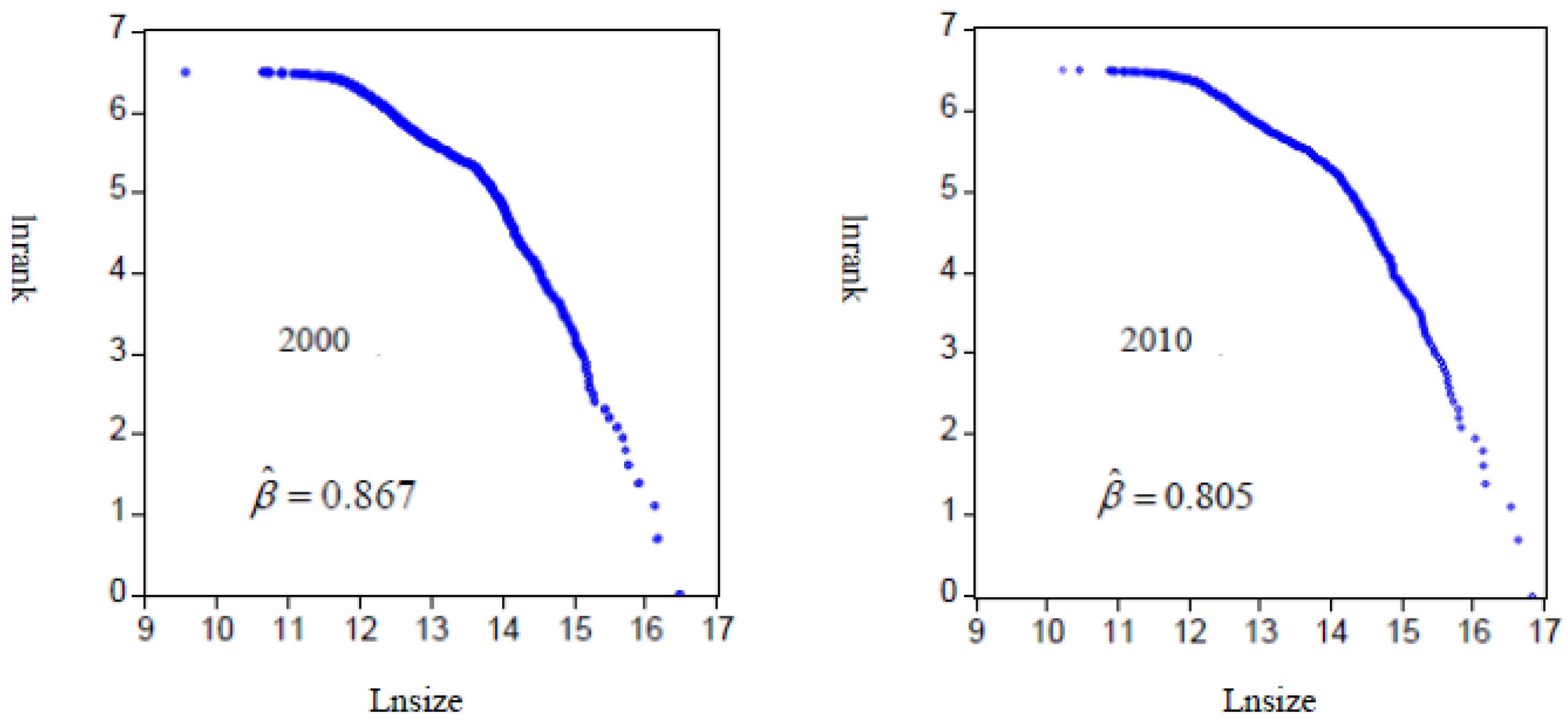
| Year | Number of Sample | Estimation | |||
|---|---|---|---|---|---|
| Constant Term () | Pareto Exponent () | Deviation () | R2 | ||
| 2000 | 663 | 16.70 *** | 0.867 *** | 0.997 | 0.879 |
| 2010 | 657 | 16.16 *** | 0.805 *** | 0.997 | 0.862 |
| Category | Economic Efficiency | “Economic-Environmental” Efficiency | ||||
|---|---|---|---|---|---|---|
| 2000 | 2005 | 2010 | 2000 | 2005 | 2010 | |
| Megacity | 0.936 | 0.872 | 1 | 0.989 | 0.977 | 0.974 |
| Large City | 1 | 1 | 1 | 1 | 1 | 0.980 |
| Type I Big City | 0.892 | 0.784 | 0.876 | 0.954 | 0.981 | 0.988 |
| Type II Big City | 0.868 | 0.754 | 0.801 | 0.961 | 0.996 | 0.995 |
| Medium-sized City | 0.738 | 0.775 | 0.752 | 1 | 1 | 1 |
| Type I Small City | 0.702 | 0.685 | 0.724 | 0.971 | 1 | 1 |
| Type II Small City | 0.505 | 0.701 | 0.722 | 0.892 | 0.881 | 0.922 |
| Mean value | 0.806 | 0.796 | 0.839 | 0.967 | 0.976 | 0.980 |
| Period | Category | Effch | Techch | Pech | Sech | Tfpch |
|---|---|---|---|---|---|---|
| 2000–2010 | Megacity | 1.175 | 1.300 | 0.968 | 1.207 | 1.475 |
| Large City | 1.000 | 1.640 | 1.000 | 1.000 | 1.640 | |
| Type I Big City | 1.127 | 1.284 | 1.064 | 1.063 | 1.411 | |
| Type II Big City | 1.017 | 1.233 | 1.003 | 1.014 | 1.250 | |
| Medium-sized City | 1.105 | 1.133 | 1.000 | 1.105 | 1.238 | |
| Type I Small City | 1.069 | 1.201 | 1.079 | 0.990 | 1.269 | |
| Type II Small City | 0.992 | 1.166 | 1.030 | 0.962 | 1.157 | |
| Mean value | 1.069 | 1.280 | 1.021 | 1.049 | 1.349 | |
| 2000–2005 | Megacity | 1.074 | 1.260 | 0.937 | 1.138 | 1.334 |
| Large City | 1.000 | 1.740 | 1.000 | 1.000 | 1.740 | |
| Type I Big City | 1.013 | 1.401 | 1.006 | 1.007 | 1.413 | |
| Type II Big City | 1.162 | 1.203 | 1.000 | 1.162 | 1.365 | |
| Medium-sized City | 1.031 | 1.078 | 1.051 | 0.980 | 1.109 | |
| Type I Small City | 1.030 | 1.218 | 1.056 | 0.975 | 1.248 | |
| Type II Small City | 0.935 | 1.288 | 1.002 | 0.933 | 1.222 | |
| Mean value | 1.035 | 1.312 | 1.007 | 1.028 | 1.347 | |
| 2006–2010 | Megacity | 1.276 | 1.341 | 1 | 1.276 | 1.617 |
| Large City | 1 | 1.54 | 1 | 1 | 1.54 | |
| Type I Big City | 1.241 | 1.168 | 1.121 | 1.12 | 1.409 | |
| Type II Big City | 1.1 | 1.178 | 1.004 | 1.096 | 1.278 | |
| Medium-sized City | 1.048 | 1.064 | 1 | 1.048 | 1.112 | |
| Type I Small City | 1.107 | 1.183 | 1.102 | 1.005 | 1.29 | |
| Type II Small City | 0.953 | 1.253 | 1.009 | 0.944 | 1.206 | |
| Mean Value | 1.104 | 1.247 | 1.034 | 1.070 | 1.350 |
| City Category | 2000–2005 | 2006–2010 | 2000–2010 | ||||||
|---|---|---|---|---|---|---|---|---|---|
| Labor | Capital | Land | Labor | Capital | Land | Labor | Capital | Land | |
| Type I Big City | 0 | 0.232 | 0.012 | 0 | 0.153 | 0.007 | 0 | 0.193 | 0.010 |
| Type II Big City | 0.017 | 0.147 | 0.04 | 0.007 | 0.210 | 0.021 | 0.012 | 0.179 | 0.031 |
| Medium-sized City | 0.072 | 0.009 | 0.085 | 0.094 | 0.026 | 0.113 | 0.083 | 0.018 | 0.099 |
| Type I Small City | 0.128 | 0.145 | 0.369 | 0.156 | 0.152 | 0.228 | 0.142 | 0.149 | 0.299 |
| Type II Small City | 0.283 | 0.137 | 0.273 | 0.237 | 0.009 | 0.306 | 0.260 | 0.073 | 0.290 |
© 2016 by the authors; licensee MDPI, Basel, Switzerland. This article is an open access article distributed under the terms and conditions of the Creative Commons Attribution (CC-BY) license (http://creativecommons.org/licenses/by/4.0/).
Share and Cite
Li, H.; Wei, Y.D.; Ning, Y. Spatial and Temporal Evolution of Urban Systems in China during Rapid Urbanization. Sustainability 2016, 8, 651. https://doi.org/10.3390/su8070651
Li H, Wei YD, Ning Y. Spatial and Temporal Evolution of Urban Systems in China during Rapid Urbanization. Sustainability. 2016; 8(7):651. https://doi.org/10.3390/su8070651
Chicago/Turabian StyleLi, Huan, Yehua Dennis Wei, and Yuemin Ning. 2016. "Spatial and Temporal Evolution of Urban Systems in China during Rapid Urbanization" Sustainability 8, no. 7: 651. https://doi.org/10.3390/su8070651