Article

Studies of the Relationship between City Size and Urban Benefits in China Based on a Panel Data Model

1
Xinjiang Institute of Geography and Ecology, Chinese Academy of Sciences, Urumqi 830011, China
2
University of Chinese Academy of Sciences, Beijing 100049, China
*
Author to whom correspondence should be addressed.
Sustainability 2016, 8(6), 554; https://doi.org/10.3390/su8060554
Submission received: 21 February 2016 / Revised: 5 June 2016 / Accepted: 7 June 2016 / Published: 15 June 2016
(This article belongs to the Special Issue Maintaining Ecosystem Services to Support Urban Needs)

Abstract

:
Policy regarding the size of cities is an important component of China’s urban policy prescription. We used a curvilinear regression model in this study to identify the optimal function and conducted curve panel data regression analysis on the panel data of the benefits of the economy, ecosystem services, and city size in China. In doing so, we obtained the regression relationship between city size and the benefits of the economy, environment, and resources of a city. Our main findings are as follows: (1) city size is not the most important factor determining a city’s benefits. However, there is a significant difference in the average city benefit between cities of various sizes; (2) city per capita GDP increase exhibited an inverted-N-shaped relationship with increasing city size, initially decreasing but subsequently increasing. The city size corresponding to the maximum value was usually higher than or close to the actual city size. Thus, it can be concluded that when a city’s population is more than 1 million, its per capita output increases; (3) a city’s resource services benefits all exhibited the trend of improving with increasing city size. This trend was particularly pronounced among cities with a population of less than 1 million; and (4) a city’s environmental services benefits exhibited an inverted-U-shaped relationship with city size, initially increasing but subsequently decreasing.

1. Introduction

In March 2014, China introduced new strategic urban planning guidelines mandating “full liberalization of the household registration restraints in townships and small cities, gradual liberalization of the restraints in cities with a population of 0.5–1 million, and strategic liberalization of the restraints in big cities with a population of 3–5 million, and strategic determination of the conditions of household registration in the big cities, and strict control the urban population in large cities with a population of over 5 million.” The new urban planning guidelines revived the discussion in China on urban size policy and its economic and ecosystem benefits.
China has experienced rapid urbanization in the last few years. According to the China Statistical Yearbook [1], the urbanization rate increased from 17.92% in 1978 to 52.57% in 2012. During this period, approximately 500 million people moved from rural areas to cities, and the number of big cities with populations of more than 1 million increased from 15 to more than 100. This rapid urbanization has been largely driven by China’s urbanization policies [2]. Thus, China’s urbanization policies, particularly policies regarding city size, have begun attracting the attention of politicians and academics. Ratified by the State Council in 1980, the Proceedings of the National Urban Planning Conference stressed that “we should control metropolitan scale, rationally develop the medium-sized cities, and actively develop small cities.” The Urban Planning Law was implemented on 1 April 1990, and the guiding principle of urban development was legally clarified, stating that “to strictly control the scale of large cities, rationally develop medium-sized cities and small cities." This law is still in effect and provides the legal basis of the government’s city size policies. However, this law has failed to meet China’s urban development needs. Therefore, development has not conformed with the aforementioned prescriptions designed by these strategic plan [3].
It is, thus, necessary to analyze the impact of China’s urban population on urban economic and ecosystem services benefits. Based on this analysis, recommendations for the optimization of urban development policy will be made to improve the rationale of decision-making in urban development and to enhance the development capacity of cities.
Rashevsky was the first to investigate city size issues and proposed a theoretical model for reasonable city size within a specific region from the perspective of the relationship between the city and the region. However, it was not until the late 1960s that more research on this topic began to emerge [4]. Tolley constructed a model demonstrating how city size affects income and cost of living, and believed that because the political preferences of government officials indirectly influenced spatial policy, optimal city size did not exist in a sub-optimal world in which externalities were not fully internalized [5]. Henderson assigned various production functions to each of the cities and found that the optimal solution was likely not the only value but was rather a range of values [6]. Camagni et al. constructed a comprehensive model to measure the reasonable size of cities, taking into account quality of life, industrial diversity, and degree of social harmony [7]. Since the 1980s, various scholars have conducted empirical studies on the benefits of city size in various countries and regions and obtained optimal city size ranges for the respective regions [8,9,10,11,12,13,14]. Meanwhile, with the continuous focus on global resources and environmental issues, the impact of resources and environment on urban development has been examined in studies of the benefits of city size. The relationships between city size and urban heat islands [15], air quality [16], resource consumption [17,18], and environmental pollution costs were quantitatively investigated [19,20].
Studies on the benefits of city size in China can be divided into two phases. The first phase began in the 1980s, when proponents of small cities and proponents of large cities began to clash. The rationale behind small cities was mainly an argument concerning “special situations of the nation and cities”. Small-cities proponents asserted that various urban problems existed in China’s large cities. Additionally, small-cities proponents argued that due to close geopolitical relationships, the cost to farmers to enter small cities was lower than it was to enter medium and large cities, thus lowering the cost of urbanization. Further, the development of rural secondary and tertiary industries can be promoted so that a large number of rural surplus laborers can be accommodated in small cities. In 1984, Xiaotong Fei published a series of investigative reports titled “Small towns but big problems” arguing that the development of small towns should be the main focus of urbanization in China [21,22],. Fei’s assertion catalyzed widespread national debates. Proponents of big cities noted the shortcomings in the arguments of the proponents of small cities stemming from having ignored the benefits of large city size, arguing that big cities have much larger scale efficiency than small cities. Based on studies of other countries’ urbanization processes, big-cities proponents believe that there exist “objective rules of advanced development of big cities” and that China should focus on developing big cities. Hu argued that the advanced development of big cities is a statistical rule and that their rapid development is a global trend [23]. Rao and Cong argued that large cities offer better economic, social, environmental, and architectural benefits than small and medium cities and that city size efficiency is an important and universal rule that should be used to accelerate urbanization [24]. Yu reemphasized that the “advanced growth of big cities” was a universal rule and believed that “developing big cities and intensive development are the only ways of urbanization in China.” Thus, the reasonable choice was to actively and selectively develop large cities [25].
The second phase of urbanization in China began in the mid-1990s, when research was no longer limited to conceptual city size and was more quantitative. Chen and Jiang used the cost-benefit curve of city size generated by Barton (an urban economist) to quantitatively analyze the panel data of 666 cities nationwide and concluded that the size of cities with maximum net scale benefits was 1–4 million, i.e., the optimal size of the city [26]. Wang and Xia noted that large cities have significant net scale benefits and that optimal city size was between 0.5–4 million, with the peak value ranging between 1 and 2 million [27]. Ma and Song argued that, except for Beijing, Shanghai, and Tianjin, three mega-cities with relatively high-scale benefits and sustainable development capacity, mega- and large cities with populations of 1–2 million and 0.5–1 million, respectively, rank high in both scale benefits and sustainable development capacity [28]. By conducting an empirical analysis using relevant city data from 1995–1996, Rao and Cong concluded that optimal city size in China is approximately 6.5 million and that technological progress and institutional innovation tend to increase the optimal size [29]. Based on the input-output differences in the three critical elements of capital, land, and labor of cities of different sizes, Yu used the entropy-DEA method and concluded that after the urban population reached 50,000, economic efficiency significantly improved, whereas cities with a population of less than 30,000 had low utilization efficiency in public facilities and poor investment returns [30]. Zheng performed the regression analysis on the actual change in the relationship between city size and per capita GDP, per capita investment, per capita net income, and per capita input-output net income and found that the reasonable and efficient size of regional major cities ranged between 1.5 and 2.7 million [31]. Yan and Feng demonstrated that accelerated growth in city size after 2000 encouraged the development of large cities [32]. Sun et al. researched the relationship between cost of production and city size of population by constructing a per unit production coat function, and finding that large cities were more productive and the optimal city population size was 4.2 million [33].
China is a resource-short country by per capita resources, where water per capita is only 1/4 of the global average and per capita arable area is 40% of the global average. The problems of resource limits become serious with the fast development of urbanization. Therefore, researches on Chinese urbanization and resource consumption have shown a rapid increase this century. Varis and Vakkilainen’s research showed that increasing demand of agricultural products, continuous deterioration of the ecological environment, and the threat of climate change would be a huge challenge to Chinese resources, and Chinese environmental pressure had already exceeded its capacity [34]. Shen et al. developed a model to describe the relationship of urbanization, economic development, and resource supply, and predicted a supply-demand relationship of resources from 2005 to 2050 [35]. Xu gave panel regressions of relationship between city size and resources efficiency [36]. Hong et al. measured the relationship between Chinese city size and energy [37]. Han et al. researched Chinese city size and PM2.5 pollution and found that there was an inverse-U-type relationship [38].
Much of the research has evaluated the economic or ecosystem services benefits of city size using description or model methods and has concluded on the individual optimal range of the scale, whereas previous studies on the relationship between city size and resources and environmental benefits were largely confined to an empirical model, but lacked rigorous statistical analysis. Additionally, due to China’s vast regions and rapid growth, the processes of urbanization and economic and social development taking place at different times and in different regions displayed significant variations. In this study, we embarked on a systematic and quantitative analysis of the benefits of economy and ecosystem services of cities in different times and regions to pursue more comprehensive and objective conclusions.
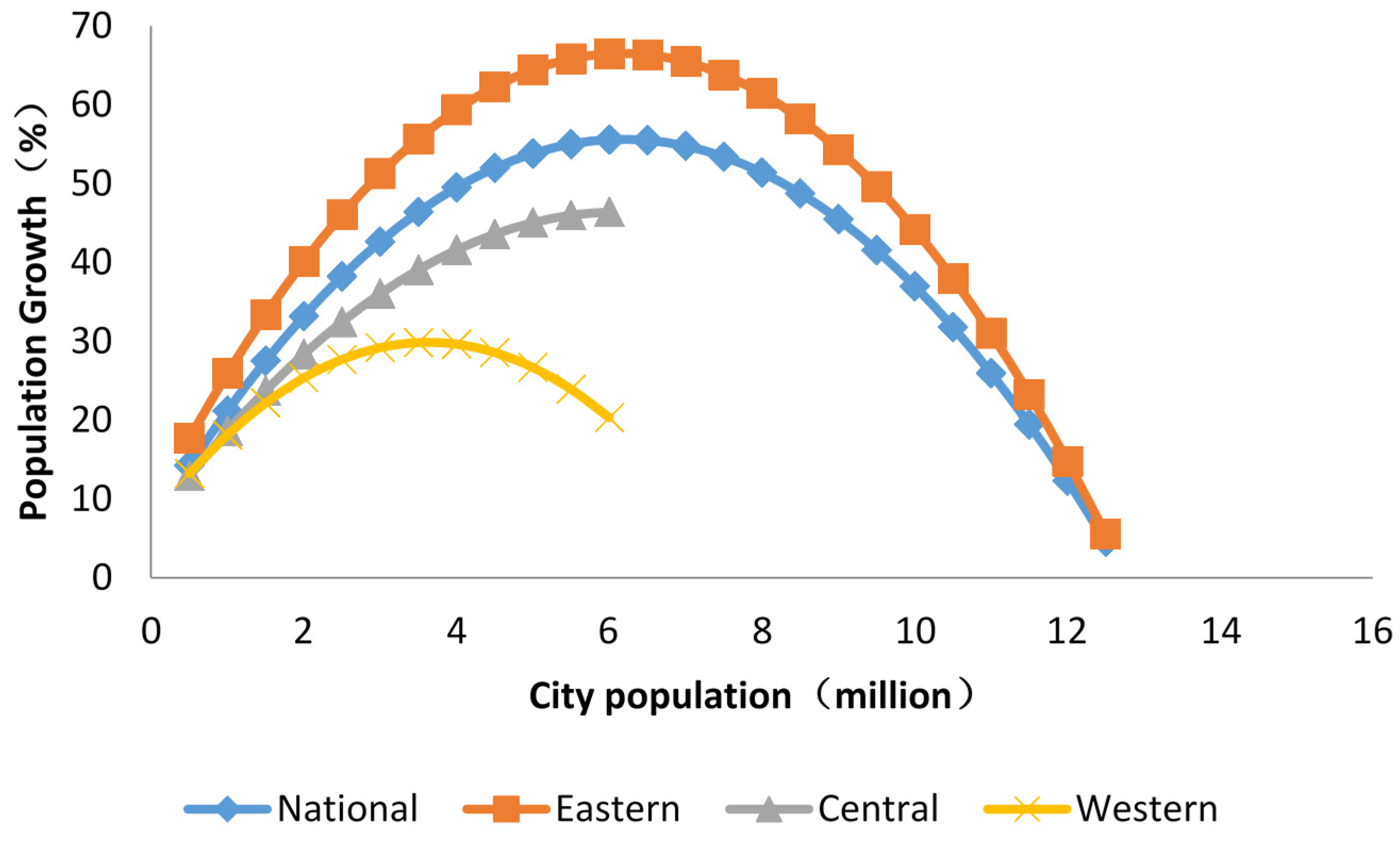
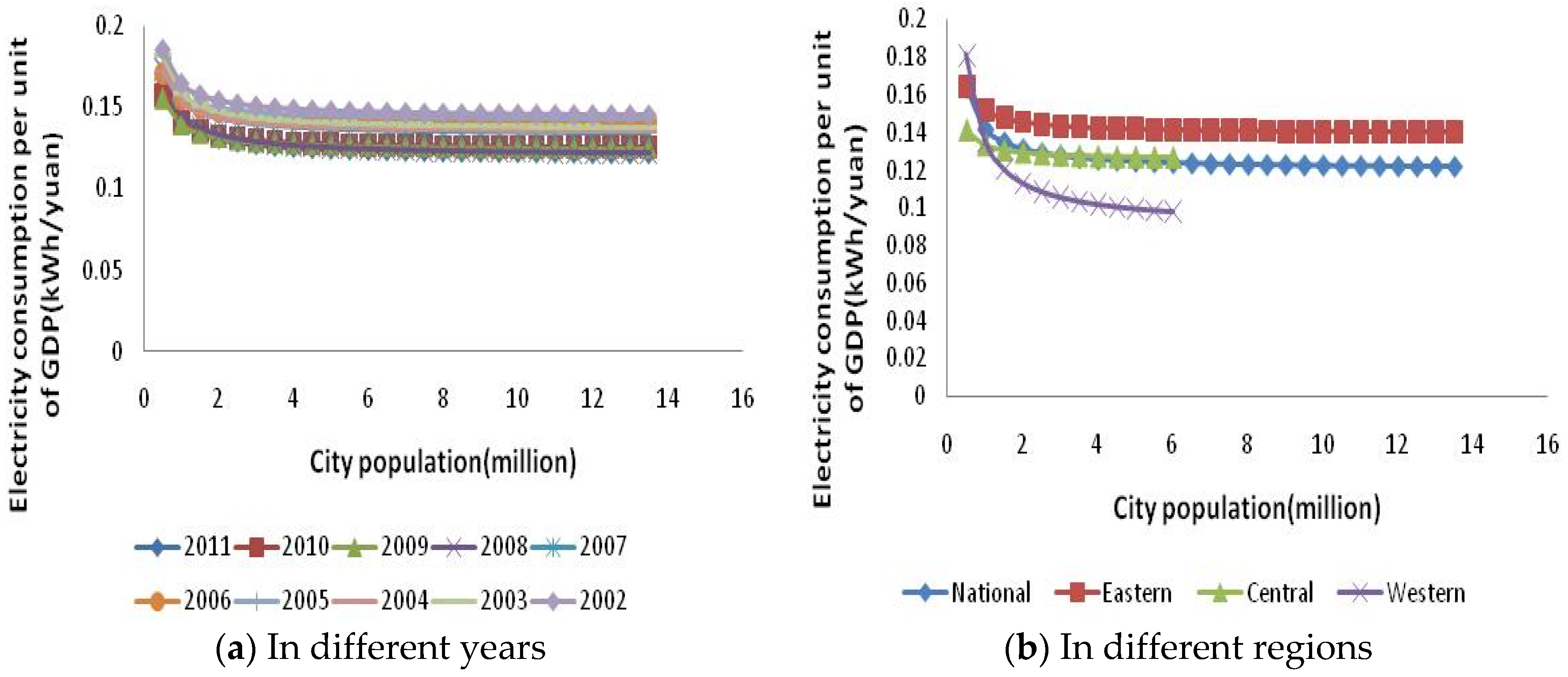
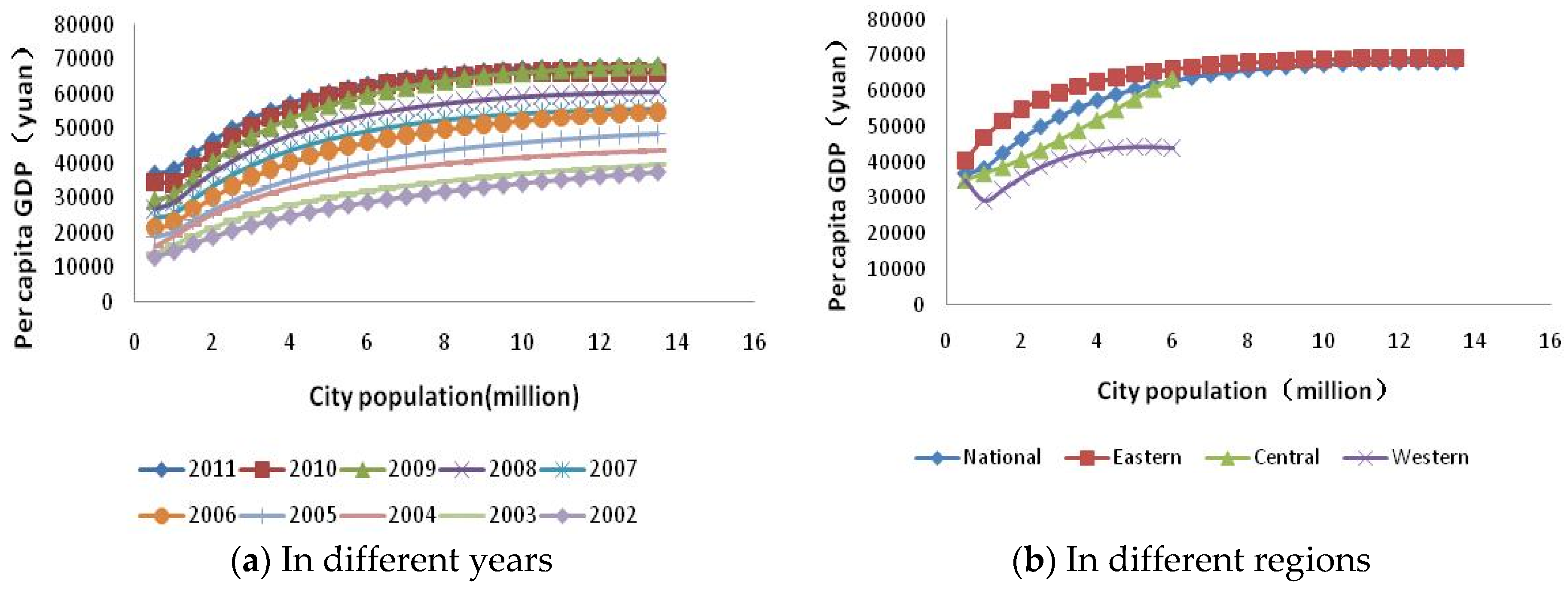
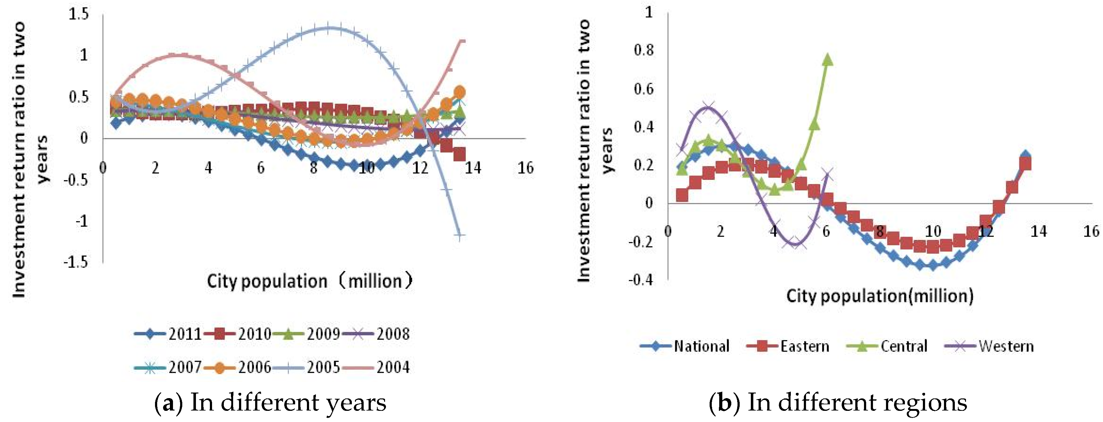
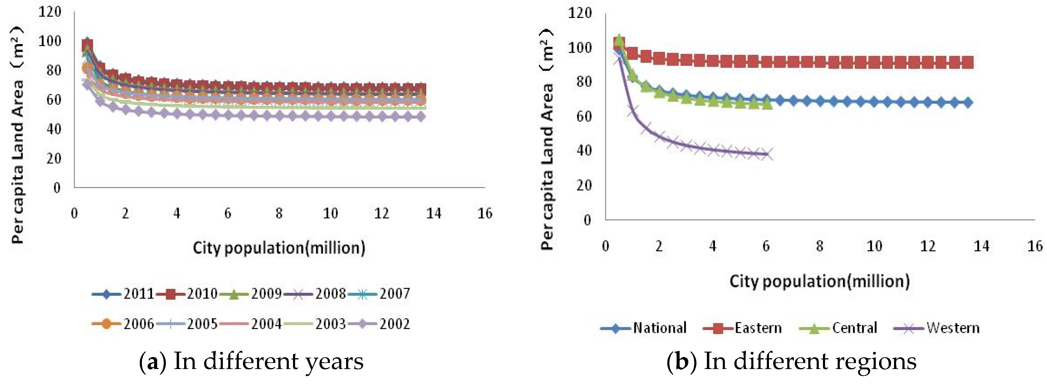
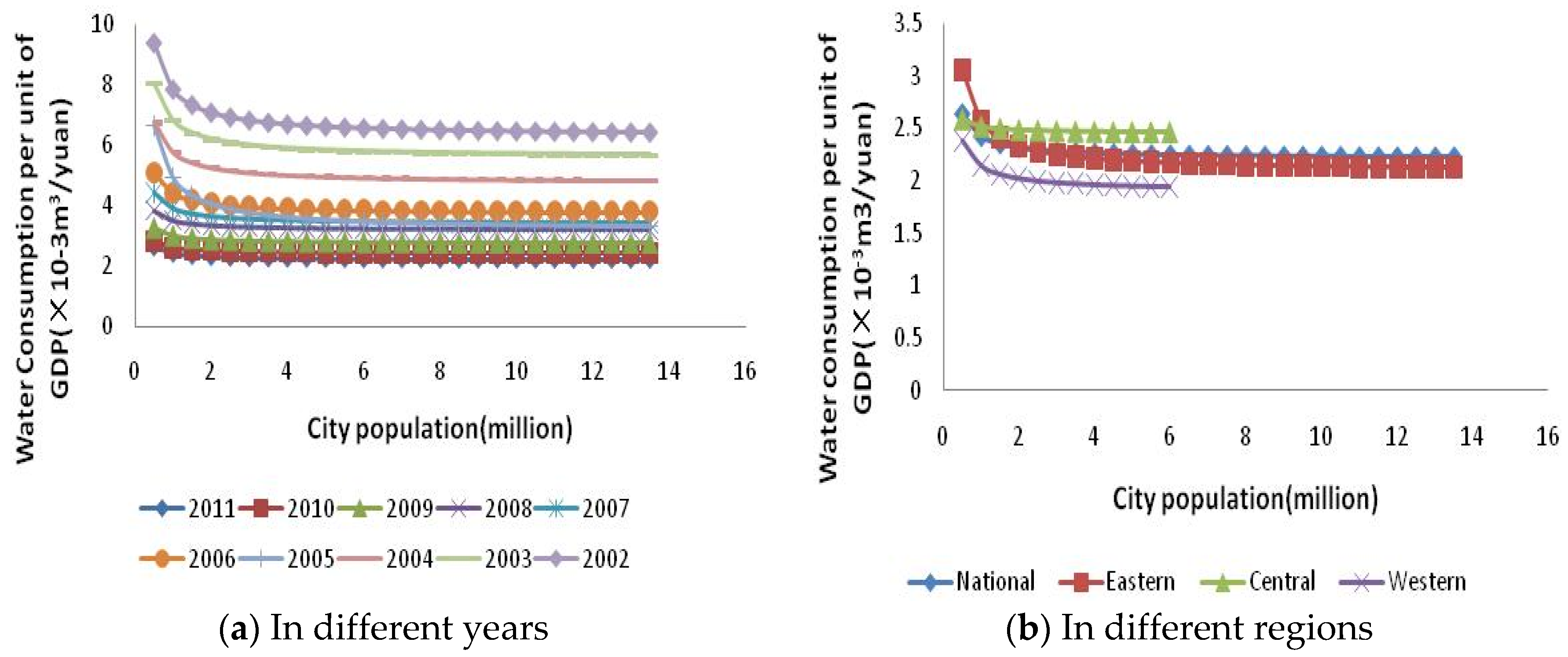
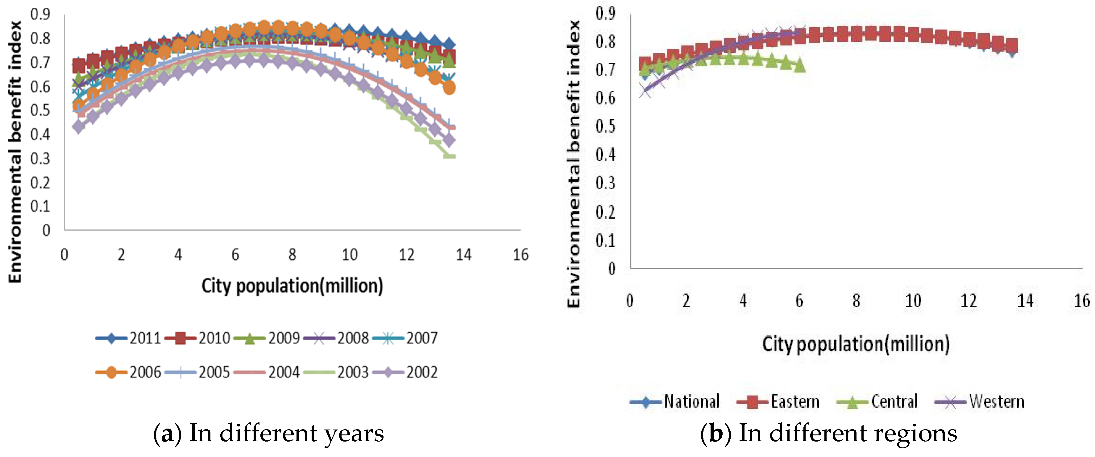
We established an index system that includes urban population growth, economic efficiency, efficiency of resources services, and environmental benefits. Population growth in 10 years was selected as a variable to avoid inter-annual fluctuations in population in the indicator of population growth. In terms of economic efficiency, per capita GDP and city investment-return ratio were used as variables. For the efficiency of resources services, per capita construction land use, water consumption per unit of GDP, and electricity consumption per unit of GDP were used as indicators. For environmental benefits, because the relevant individual indicator was largely irrelevant to this study, an environmental benefits index consisting of per capita green area, treatment rate of industrial solid waste, sewage treatment rate, and treatment rate of domestic garbage was used as the indicator.
Based on the models used in previous studies, in this study population growth and economic benefits were screened through linear regression to determine the most realistic regression model, then the regression analysis using the panel data was conducted to estimate the coefficients for the related indicators and to determine the optimal range of city size and the problems that actually exist. Temporal and spatial changes in the correlation coefficient and their practical significance were also analyzed. Due to significant differences in natural conditions and development status among different regions in China, the regression analysis was performed on individual cities throughout Eastern, Central, and Western China, to arrive at more detailed and realistic conclusions.
A review and summary of previous results will be presented in the next section. The relevant models used in this study will be discussed in Section 2. The regression analysis on each of the indicators at different times and in different regions will be conducted and the differences at different times and different regions will be discussed in Section 3. In the final section, the main conclusions and new discoveries made in this study, as well as appropriate recommendations for Chinese urbanization policy based on our findings, will be presented.

2. Methods and Data

2.1. Models and Methods

2.1.1. Regression Model of City Size and Population Growth

This relationship is measured to find out cities of which size grows fastest. The function between city size and population growth would be an inverted-U-shaped relationship: when the city size is small, the growth rate of the population would become higher with the increase of city size; when city size passes an optimal point, the growth would go down with the increase of city size. That is:
y = ax3 + bx2 + cx + d
where y is the population growth of city, x represents the population, and a, b, and c are parameters to be estimated.

2.1.2. Regression Model of City Size and Urban Economic Benefits

Alonso argued that the aggregate economic level of a city is positively correlated with the unitary items of city size but negatively correlated with the quadratic items of city size [39]. Based on this argument, the quadratic function model of city size and the aggregate economic level were established using the following function:
UAEi = a + bPOPi + cPOPi2, b > 0, c < 0
where UAEi represents the aggregate economic level of the city and POPi represents the urban population size. a is a constant term, and b and c are regression coefficients. If c is negative, it would be an inverted-U-shaped relationship. The optimal city size can be obtained by partial differential:
dUAEi/dPOPi = b + 2cPOPi = 0
POPi* = −b/2c
Alonso’s model offered a way to find out an optimal city population for its economic efficiency, but as both economy and population usually have an exponential growth, a quadratic function may not express their relationship. According to the modified Douglas production function, Liu and Yang proposed the following logarithmic regression equation [40]:
lnYit = lnA0 + git + αlnKit + βlnLit + γlnUit + δlnZit + ui + ε,
i = 1,…, N; t = 1,…, T,
where i represents the ith city, t represents t year, and A0 is the initial productivity level. Yit, Kit, Lit, and git denote physical capital, labor, and the rate of technological progress of the i-th city t-year GDP. Uit is the city size situation represented by the population of the city area and the urbanization rate, and Zit represents the allocation situations of city resources. g represents rate of technological progress, α and β represent capital elasticity and labor elasticity, respectively, γ represents the scale benefits of the city, and δ represents the economic benefits of resource allocation.
Wang and Xia introduced quadratic items of the city logarithmic scale, expressed as [27]:
lnY = C + gT + αlnK + (1 − α)lnL + Τ1lnU + Τ2(lnU)2
where Y, K, L, and U represent GDP, capital, labor, and city size, respectively. α and 1 − α are the output elasticities of capital and labor, respectively. C is the productivity level, g is the growth rate of productivity, T is the time effect, and T1 and T2 are the city size benefits where the portion in the function that is related to city size is Τ1lnU + Τ2(lnU)2.
Zheng proposed that city size and urban benefits should be a cubic function curve [31]:
y = ax3 + bx2 + cx + d
where y is the urban per capita net income or urban investment-benefit ratio, x is the urban population size, and a, b, c, and d are coefficients to be determined. This model implies that there may be more than one extreme point, and an optimal value may not exists. According to this model, the economic benefits of the city would increase, and subsequently decrease, with increasing population growth, assuming an inverted-N-shaped curve. Yaping Zheng used this model to analyze the scale benefits curve for cities in China in 2004.

2.1.3. Regression Model of City Size and Urban Resources Services Utilization Efficiency

Xu speculated that with the aggregation of resources during the early phases of a city’s expansion, the scale benefits of resource utilization become increasingly significant, output per unit resource increases continuously, and per capita resource consumption exhibits a declining trend. As a city expands to a certain scale, the scale non-benefits of resource aggregation become increasingly obvious and output per unit resource exhibits a decreasing trend [36]:
y = a + bx + cx2, c < 0
where y is output per unit resource, x represents the population, and a, b, and c are parameters to be estimated.
However, as not all resources are used for economic aids but for basic urban operations. We can assume that the amount of resources consumed per unit of GDP is divided into two parts: the city’s constant cost, i.e., the resources must be consumed regardless of the size of the city, which are primarily the resources consumed by public services, and the individual’s constant cost, i.e., the extra amount of resources required to produce one unit of gross production. Thus:
RPG = a + b/x
where RPG is the amount of resources consumed per unit GDP, X is the population size, and a and b are coefficients to be estimated.

2.1.4. Regression Model of City Size and Urban Benefits of Environmental Services

Grossman and Krueger used the environmental Kuznets curve (EKC) to measure the relationship between economic development and environmental quality, arguing that economic development and environmental quality assume an inverted-U-shaped relationship. In other words, the environment deteriorated and subsequently improved [41]:
E = a + bx + cx2, c < 0
where E represents environmental quality, x is the economic development level, and a, b, and c are the parameters to be estimated.
Some researchers think the relationship is more complicated. Xu argued that it is difficult for a small city to support the normal operation of waste treatment companies. Therefore, with the expansion of city scale, environmental quality improves. However, after reaching a certain threshold value, the further expansion of the city produces a further increase in costs for pollution treatment. Thus, economic development and environmental quality assume an inverted-N-shaped relationship [36]:
E = a + bx + cx2 + dx3, c > 0, d < 0

2.1.5. Panel Data Regression

Panel data refer to the multidimensional time-series data obtained by continuous observation of the samples at different moments. This multi-dimensional data can integrate more information and has been widely applied in economics. The basic assumption of the panel data regression is the homogeneity of parameters. These parameters are generated by the probability distribution function of a certain function. The general panel data regression model can be expressed as:
Yit = ait + bit’xit’ + uit (i = 1,…, N; t = 1,…, T)
where ait is a constant term, xit’ is the vector of exogenous variables, bit’ is the vector of parameters, N is the total number of interface units, and T is the total number of times. The random disturbance term uit is independent and has an average of zero. The identical variance ait can be divided into the overall effect, the section effect, and the time effect:
ait = a + δi + ηt
a, δi, and ηt are the overall effect, time effect, and section effect, respectively.
Reviews of the panel data can only be directly used in linear regression. However, for a function that can be converted into a linear regression via linear transformation, regression can be performed after the transformation.
Therefore, we use the data of a single year (2011) to test the relevant function models, choose the most appropriate model, and conduct multi-year and multi-region panel data regression on the corresponding panel data via linear transformation to generate intersectional regression parameters at different times and in different regions, and to further analyze their variation features to draw relevant conclusions.

2.2. Data and Data Processing

We retrieved a total of 10 panel data indicators from the China City Statistical Yearbook (2002–2011) [1], including population in the municipal district, GDP, urban fixed asset investment, constructed area, water consumption, electricity consumption, green area, recycling rate of industrial solid waste, harmless disposal rate of domestic waste, and sewage treatment rate of 289 cities above the prefecture-level. In all, 271 valid cities were used in the analysis after deleting 18 cities that had missing data. The deleted cities are listed in Table 1.
Data on population, per capita GDP, urban investment-return ratio, water consumption per unit of GDP, electricity consumption per unit of GDP, per capita green area, per capita constructed area, and environmental quality index were generated by calculation. The calculation methods are presented in Table 2. The economic data, including investment and GDP, were adjusted equivalent to the 2002 constant price. In calculating the investment return of the city, considering the delay between the investment and the return during the investment process, we examined newly-added GDP data from 2011 and the correlations between the fixed asset investments in 2010, 2009, and 2008 and found that the correlation between investment and return was the highest in the two-year term investment (Table 3). Therefore, we used the newly added GDP and fixed asset investment made two years prior to calculate the investment-return ratio. In calculating the environmental quality index, we first transformed the green area per capita to a dimensionless value of between (0, 1) using the deviation standardized conversion. Since the factor analysis indicated that the correlation among the four indicators was low (Table 4), the arithmetic average method was used to compute the environment index.
Based on the division method of China’s seventh five-year plan, the cities were divided into three regions: eastern, central, and western, of which 99 were eastern cities, 98 were central cities, and 74 were western cities. The regional panel data regression was then performed on each of the regions. The details of the regions are presented in Table 5.

3. Results and Analysis

3.1. City Size and Population Growth

It can be observed that although the coefficients of some models were significant, the correlation coefficients were always relatively low, suggesting that city size was not the main factor affecting urban population growth. Model y = ax2 + bx + d had both an optimal correlation coefficient and an optimal coefficient significance. Thus, urban population growth and urban population size from 2002 to 2011 only exhibited a weak logarithmic regression relationship.
As shown in Figure 1, the coefficients of the quadratic terms for the eastern, central, and western regions were all negative indicating that, in the last 10 years, the city size and population growth rates exhibited an inverted-U-shaped relationship, first increasing and subsequently decreasing. This result suggests that city size had both promoting and limiting effects on urban development. When city size was small, the expansion of the city promoted urban development, but when city size reached a certain threshold scale, city size played the major role of limiting urban development. Nationally, the average growth percentage of the population in the past 10 years was 17.96%, and the extreme point of the proportional growth rate was 6,185,700, with an extreme growth percentage of 55.62%, i.e., with more than one half of a population increase in the previous 10 years. Regionally, the extreme points of the proportional growth rate of the eastern and central regions were similar, with faster population growth in the eastern region. The extreme point of the proportional growth rate of the western region was small at approximately 3,628,800, with slower population growth. This growth rate is primarily attributed to the western region’s poor ecology (limited environmental capacity) and secondarily to its low level of economic development due to the scale benefits of economy not having been fully realized.

3.2. City Size and Economic Benefits

3.2.1. City Size and Per Capita GDP

The correlation coefficient between urban per capita GDP and city size was similarly low, less than 0.1, indicating that city size was not the determining factor of per capita income. In the regression correlation coefficients of all of the models, y = a(lnx)3 + b(lnx)2 + c(lnx) + d and Iny = a(lnx)3 + b(lnx)2 + c(lnx) + d had the highest correlation coefficients, but the coefficient a of the latter did not pass the test, and the significance of coefficients b and c were both low. Therefore, y = a(lnx)3 + b(lnx)2 + c(lnx) + d was deemed as the optimal regression model of urban per capita income and city size. In other words, the urban per capita income and logarithm of city population size displayed a cubic function relationship.
In each of the years, the coefficient of the cubic item for the national model was negative but that of the quadratic item was positive, indicating that the theoretical relationship between urban per capita income and city size showed an inverted-N-shaped curve. When the population was smaller than 500,000, the city’s per capita output tended to decline with increasing city size, indicating that the city size under 500,000 did not produce significant economies of scale benefits. When the population was greater than 500,000, the city’s per capita output began increasing with population increases. In the first three years, each of the items was insignificant, but the coefficients became increasingly significant with time and the inverted-N-curve relationship became increasingly apparent. As shown in Figure 2a, in the last 10 years, the city’s per capita output accelerated in similarly sized cities. The city size corresponding to the minimum of the city’s per capita output rose slowly, from 475,700 in 2002 to 634,600 in 2011. City size corresponding to the maximum of a city’s per capita output was maintained above 10 million, and only in the last two years did some cities reach the scale corresponding to the theoretical maximum value. These results demonstrate that city size did not achieve optimal economy for a long time, and only in the last two years did some mega-cities begin to reap optimal economic benefits.
As shown in Figure 2b, the highest per capita output in 2011 was produced in eastern coastal cities. Moreover, city size corresponding to the minimum value was small, whereas city size corresponding to the maximum value was large, indicating that urban economic benefits were generally positive in the eastern region, which correlates to the greater economic development of the region. The central region has not yet formed a clear inverted-N-shaped relationship. However, on the range of the existing urban scale, the per capita output of the central region was lower than that of the eastern region, but higher than that of the western region. In the western region, not only was the urban per capita output low but the per capita output and the city size corresponding to the maximum value were also low at only 5.17 million. Only a limited number of cities in the western region can attain this city size. This is largely due to the fragile ecological conditions in the western region that renders it difficult to support large cities. Additionally, outdated technology has rendered the economic agglomeration benefits insignificant. Therefore, from the perspective of economic efficiency, city size in the western region should not be too large, and the optimal city size should be rationally determined based on ecological carrying capacity in the region.

3.2.2. City Size and Investment Returns

Although the correlation coefficient of the model of y = alnx3 + blnx2 + clnx + d and y = alnx2 + blnx + c was relatively high, the significance test of the coefficients failed. Thus, the model y = ax3 + bx2 + cx + d was chosen. In other words, urban investment returns and city size exhibited a cubic function relationship.
As shown in Figure 3a, except for a few years, the theoretical relationship between urban investment returns and city size all exhibited an N-shaped curve. When city size was smaller than 2 million, urban investment returns displayed an increasing trend, but when city size exceeded 3 million, investment returns began to decline until city size reached more than 9 million. However, even for the current mega-city with a population of more than 10 million, investment efficiency was still low. That is, for existing cities, urban investment returns and city size exhibited an inverted-U-shaped relationship, initially increasing and subsequently decreasing. This result shows that although mega-cities had higher per capita economic levels, a fixed assets investment was still more advantageous for cities with populations of approximately 2 million. This finding corresponds to the cities’ more rapid growth stage, when infrastructure was in its infancy. Therefore, the state should invest in general cities with rapid development rather than in mega-cities.
Regionally (Figure 3b), the city size corresponding to the maximum value was large in the eastern region at 2,779,000, and the city sizes of the central and western regions were relatively smaller at 1,502,100 and 1,409,100, respectively. These figures can be largely attributed to the higher level of urbanization in the eastern cities and greater demand for fixed assets investment. It is worth noting that the sizes of the cities corresponding to the minimum investment return in the central and western regions were all small at only 4.05 million and 4.78 million, respectively, whereas city size reached 9.9154 million in the eastern region. This indicates that the current level of economic development of the central and western mega-cites, characterized by nascent economies and low levels of technology adoption, has precluded these cities from yielding large investment returns. From the investment return viewpoint, the size of large cities in the central and western regions should be below 5 million.

3.3. City Size and Resources Services Efficiency

3.3.1. City Size and Per Capita Land Area

Model y = a/x + d had both an optimal correlation coefficient and an optimal coefficient significance. Therefore, there was a linear relationship between the per capita land area and the reciprocal of city population size. The larger the city, the more savings in per capita land area. Urban land use can be divided into two parts: land area that does not change with population changes, primarily the area occupied by public facilities, equivalent to coefficient a in the formula, and the land area that linearly increases with population increases, including residential areas, productive land area, and areas for other public service facilities, equivalent to constant d in the formula.
As shown in Figure 4a, in the last 10 years, the per capita residential areas in cities of varying scale all increased, from less than an average of 50 square meters to nearly an average of 70 square meters. The curve for each of the years shows the decreasing trend in per capita land use with increasing city size. The decreasing trend was more obvious in cities with populations of less than 1 million. This indicated that big cities were more intensive in their land use. At the same population level, prioritizing the development of cities with populations of more than 1 million would help conserve more land.
It can be seen from Figure 4b that the per capita land area in eastern cities reached more than 90 square meters, a significantly higher figure than those reached in the central and western cities, which was associated with higher living standards in the eastern region and narrower plain areas in the central and western regions. Additionally, per capita land area in the western region decreased more rapidly with increasing city size, being only 40 square meters per capita in the metropolises, more than two times the size of the medium and small cities in land use efficiency. This result was attributed to land use efficiency in large cities in the western region and to land use inefficiency in many medium and small cities in the western region, which often included wide streets and city squares that wasted land. In large cities, the land was usually in short supply and, thus, less of it was wasted. Therefore, in the western region, large cities with more than 1 million residents are encouraged to further develop themselves, and the supervision of the planning of medium and small cities should be strengthened to improve land use efficiency.

3.3.2. City Size and Water Consumption per Unit of GDP

The reciprocal model better represents the regression relationship between a city’s water consumption per unit of GDP and city size. It can be seen in Figure 5a that city water consumption per unit of GDP rapidly declined over the last 10 years, from an average of 7 × 10⁻³ m3/yuan to an average of 2 × 10⁻³ m3/yuan. Cities with a population of less than 1 million saw the most remarkable decline, whereas small cities had higher water consumption per unit of GDP. Large cities used less water per unit of GDP, but when the population surpassed 1 million, the difference in water consumption per unit of GDP among cities diminished, and water consumption per unit of GDP did not change significantly with increasing city size.
As shown in Figure 5b, water consumption per unit of GDP exhibited relatively little variation among cities in the same region. Cities in the central region had the highest water consumption per unit of GDP, being nearly 2.5 × 10⁻³ m3/yuan, largely due to the paucity of industrial technology in the central region that resulted in high water consumption. There exists large water-saving potential in cities in the central region, and industrial water-saving technology innovation should be strengthened. Cities in the western region consumed the least amount of water per unit of GDP, below 2.0 × 10⁻³ m3/yuan, indicating that the ecological and environmental constraints under which western cities operate has gradually prompted them to create water-saving industrial infrastructure and development models. Water-use mechanisms and more water conservation awareness would play a key role in the long-term development of the western regional cities.

3.3.3. City Size and Energy Consumption per Unit of GDP

The reciprocal model remained the optimal model. As shown in Figure 6a, the electricity consumption per unit of GDP has slowly declined over the last 10 years, from 0.15 kwh/yuan in 2002 to 0.13 kwh/yuan in 2011, indicating that Chinese cities have significantly reduced energy consumption. When the population was below 1 million, electricity consumption per unit of GDP dramatically decreased with increasing city size, but the decrease slowed in cities with more than 1 million residents. Eastern cities (Figure 6b) consumed the highest amount of electricity. Large cities consumed 0.14 kwh/yuan per unit of GDP, and small and medium cities consumed 0.16 kwh/yuan per unit of GDP. Electricity consumption per unit of GDP in the central and western cities decreased, with large western cities exhibiting consumption levels as low as or even less than 0.10 kwh/yuan per unit of GDP. The decrease in electricity consumption is mainly because eastern cities host many of the country’s manufacturing firms, which imparts to these cities a high potential for energy conservation. Deploying improved energy technologies in the eastern region and developing the manufacturing industry in the central and western regions can help narrow the regional gap in electricity consumption.

3.4. City Size and Urban Benefits Environmental Services

Although the cubic regression function had the highest correlation coefficient, the correlation coefficient did not pass the significance test. Therefore, the quadratic model was the optimal model. The quadratic items in the function were all negative, meaning that urban environmental services benefits and city size had an inverted-U-shaped curve relationship. Meanwhile, the correlation coefficient of the panel data regression of urban environmental benefits and city size was relatively high, greater than 0.3. These results stem from the fact that city expansion can promote the management of environmental pollution. However, beyond a certain limit, the deterioration of urban pollution would exceed the management capacity, leading to a decline in environmental benefits.
Figure 7a shows that (1) the overall environmental services benefits of cities in China have continuously increased over the past 10 years, largely due to increased investment in environmental management stemming from greater economic development; (2) the environmental services benefits of cities of various sizes have converged; (3) city sizes corresponding to the extreme points of environmental benefits were distributed in the range of 6.5–8.5 million; and (4) city size corresponding to the extreme point of environmental services benefits steadily increased over the last 10 years, indicating that in terms of environmental benefits, only a few mega-cities need to restrict city size, whereas the majority of cities have not reached their optimal sizes. Relative to urban per capita GDP, city size corresponding to the maximum value of urban environmental services was slightly smaller, indicating that although mega-cities may improve economic efficiency, they create environmental problems.
According to Figure 7b, cities in the eastern region had higher environmental benefits, with an average of more than 0.7. City size corresponding to the maximum value of urban environmental benefits was also large, at 8.45 million, followed by cities in the western region, with an optimal size of 6.23 million. The environmental benefits of cities in the central region were the lowest and had the lowest optimal sizes at 3.54 million. These results are due to the central region’s long history of environmentally- and technologically-deficient industrial development. Additionally, these results demonstrate that there is a dire need to control urban pollution in the central region, particularly by improving the technical capabilities of its old industrial bases.

4. Conclusions

Based on the above analysis, we draw the following conclusions:
(1)
The regression correlation coefficients of the indicators were not very high, demonstrating that city scale was not the most important factor in determining the benefits of a city. However, there was a significant difference in the average benefits of cities among cities of various sizes. In terms of the indicators, the correlation between city size and a city’s economic benefits was low, whereas the correlation between city size and a city’s environmental benefits was high, indicating that instead of controlling urban scale, urban policy should focus on improving a city’s benefits by nurturing, among other things, the urban system and urban competitiveness.
(2)
City per capita GDP decreased with increasing city size, subsequently increased, and decreased again, exhibiting an inverted N-shaped relationship. The city size corresponding to the maximum value was often higher than, or close to, the existing maximum city size. Thus, it can be argued that when a city’s population exceeds 1 million, its per capita output increases with increasing city size. However, in terms of investment benefits, the trend increased first, subsequently decreased, and increased again. Few cities can reach the scale of the second increase. Therefore, the trend of city size and investment benefits increase first, then decrease. It is believed that the maximum investment benefits were achieved when the city sizes were 2.77 million, 1.5 million, and 1.46 million in the eastern, central, and western regions, respectively.
(3)
City resources services efficiency improved with increasing city size. When the population was less than 1 million, the trend was more profound, and when the population was more than 1 million, the increase in efficiency slowed. City environmental benefits and city size exhibited an inverted-U-shaped relationship. The optimal sizes were 8.45 million, 3.54 million, and 6.23 million for cities in the eastern, central, and western regions, respectively.
Based on the above conclusions, we make the following recommendations:
(1)
A more relaxed and targeted population control policy should be implemented. In regions with good environmental conditions, such as the eastern region, population growth in cities with more than 8 million residents should be restricted. In the central and western regions, optimal city size should be determined based on local ecological carrying capacity. For those cities that have not realized their optimal urban scale, the residency policy should be opened to encourage the population to shift to large cities to achieve better economic and environmental benefits.
(2)
Urban investment should be tilted toward smaller cities. In the eastern region, investment should focus on cities with a population of 2–5 million, and in the central and western regions, investment should focus on cities with a population of 1–3 million. In this way, higher investment returns would be realized, and healthy and sustainable development would be maintained. Meanwhile, the difference in public services facilities among cities of various sizes would be reduced, encouraging a more balanced distribution of the population.
(3)
Appropriate countermeasures can be developed based on the outstanding problems in cities in different regions. The main problems found in eastern cities were fewer benefits and, in mega-cities, high energy consumption. Thus, the population in mega-cities should be dispersed by building satellite towns, transferring manufacturing to the surrounding region, and establishing convenient intercity transportation systems. Carbon emissions should be reduced by upgrading the industrial infrastructure. Central cities in the central region were more complex, exhibiting three major problems: low levels of urban economic development, backward industrial technologies, and heavy pollution. These three problems interacted and restrained the enhancement of the scale benefits of cities. Through investment and the development of appropriate policies, the old industrial bases should be technologically upgraded to improve economic efficiency, reduce pollution, and increase the potential for urban development. Western cities had good resource and environmental benefits but were limited by resource constraints, leading to low levels of economic development and a low potential for expanding the urban scale. These cities should continue following a development model emphasizing the strengthening of resource conservation and the maximization of urban efficiency under limited resources and sub-optimal environmental conditions.
In this study, the relationship between city size and the economic, resource, and environmental benefits of cities in different regions in China was discussed within the context of the Chinese government’s city size policies. These policies not only have instructive significance for Chinese urban development but also for urban development policies in other developing countries. Since the results were drawn from the regression relationship using a statistical method, the mechanisms that governed the relationship, such as urban traffic, quality of services, and human well-being, have not been addressed. An in-depth study of the interaction between city size and urban benefits using typical cases should be conducted.

Author Contributions

Wenbiao Zhang and Degang Yang gave the idea and conceived the framework; Wenbiao Zhang analyzed the data; and Wenbiao Zhang and Jinwei Huo wrote the paper.

Conflicts of Interest

The authors declare no conflict of interest.

Appendix

Table A1. Fitting degree of regression analysis of population growth and city size of China, 2011.
ModelCorrelation CoefficientSig. of Coefficient aSig. of Coefficient bSig. of Coefficient c
y = ax + d0.0150.046
y = ax2 + bx + d0.0450.0040.000
y = ax3+bx2 + cx + d0.0500.2490.1040.009
Y = alnx + d0.0380.001
y = a(lnx)2 + blnx + c0.0400.4740.279
y = a(lnx)3 + b(lnx)2 + clnx + d0.0370.2530.2730.330
Table A2. Fitting degree of regression analysis of GDP per capita and city size of China, 2011.
ModelCorrelation CoefficientSig. of Coefficient aSig. of Coefficient bSig. of Coefficient c
y = ax + d0.0510.000
y = ax2 + bx + d0.0540.1840.004
y = ax3 + bx2 + cx + d0.0510.7730.9600.273
y = alnx + d0.0600.000
y = a(lnx)2 + blnx + c0.0640.2160.476
y = a(lnx)3 + b(lnx)2 + clnx + d0.0710.0560.0450.045
lny = alnx + d0.0590.000
lny = a(lnx)2 + blnx + c0.0650.0980.057
Iny = a(lnx)3 + b(lnx)2 + clnx + d0.0710.1020.0770.072
Table A3. Fitting degree of regression analysis of investment returns and city size of China, 2011.
ModelCorrelation CoefficientSig. of Coefficient aSig. of Coefficient bSig. of Coefficient c
y = ax + d0.0010.280
y = ax2 + bx + d0.0100.0610.031
y = ax3 + bx2 + cx + d0.0210.0430.0200.005
y = alnx + d0.0180.016
y = a(lnx)2 + blnx + c0.0250.1840.046
y = a(lnx)3 + b(lnx)2 + clnx + d0.0260.0780. 7340.024
Table A4. Fitting degree of regression analysis of per capita land area and city size of China, 2011.
ModelCorrelation CoefficientSig. of Coefficient aSig. of Coefficient bSig. of Coefficient c
y = ax + d0.0060.205
y =ax2 + bx + d0.0170.0870.036
y = aX3 + bx2 + cx + d0.0500.0020.0010.000
y = a/x + d0.0980.000
Table A5. Fitting degree of regression analysis of water consumption efficiency and city size of China, 2011.
ModelCorrelation CoefficientSig. of Coefficient aSig. of Coefficient bSig. of Coefficient c
y = ax + d0.0010.546
y =ax2 + bx + d0.0050.3320.256
y = ax3 + bx2 + cx + d0.0050.7330.6120.407
y = a/x + d0.0120.075
Table A6. Fitting degree of regression analysis of electricity consumption efficiency and city size of China, 2011.
ModelCorrelation CoefficientSig. of Coefficient aSig. of Coefficient bSig. of Coefficient c
y = ax + d0.0150.042
y = ax2 + bx + d0.0250.0970.017
y = ax3 + bx2 + cx + d0.0270.5590.3850.105
y = a/x + d0.0330.003
Table A7. Fitting degree of regression analysis of environmental benefit and city size of China, 2011.
ModelCorrelation CoefficientSig. of Coefficient aSig. of Coefficient bSig. of Coefficient c
y = ax + d0.0390.001
y = ax2 + bx + d0.0530.0440.001
y = ax3 + bx2 + cx + d0.0590.1130.009
y = alnx + d0.0010.611
y = a(lnx)2 + blnx + c0.0090.2440.248
y = a(lnx)3 + b(lnx)2 + clnx + d0.0090.2440. 7310.272

References

  1. CNKI. China City Statistical Yearbook (2002–2011). Available online: http://tongji.cnki.net/kns55/Navi/HomePage.aspx?floor=1&id=N2010042092&name=YZGCA (accessed on 27 November 2014).
  2. Zhou, S.; Dai, J.; Bu, J. City Size Distributions in China 1949 to 2010 and the Impacts of Government Policies. Cities 2013, 32, S51–S57. [Google Scholar] [CrossRef]
  3. Garmestani, A.S.; Allen, C.R.; Bessey, K.M. Time-Series Analysis of Clusters in City Size Distributions. Urban Stud. 2005, 42, 1507–1515. [Google Scholar] [CrossRef]
  4. Rashevsky, N. Contributions to the Theory of Human Relations: VII. Outline of a Mathematical Theory of the Sizes of Cities. Psychometrika 1943, 8, 87–90. [Google Scholar] [CrossRef]
  5. Tolley, G.S. The Welfare Economics of City Bigness. J. Urban Econ. 1974, 1, 324–345. [Google Scholar] [CrossRef]
  6. Henderson, J.V. Efficiency of Resource Usage and City Size. J. Urban Econ. 1986, 19, 47–70. [Google Scholar] [CrossRef]
  7. Camagni, R.; Capello, R.; Caragliu, A. One or Infinite Optimal City Sizes? In Search of an Equilibrium Size for Cities. Ann. Reg. Sci. 2013, 51, 309–341. [Google Scholar] [CrossRef]
  8. Carlino, G.A. Manufacturing Agglomeration Economies as Returns to Scale: A Production Function Approach. Pap. Reg. Sci. 1982, 50, 95–108. [Google Scholar] [CrossRef]
  9. Clark, D.; Kahn, J.R.; Ofek, H. City Size, Quality of Life, and the Urbanization Deflator of the GNP: 1910–1984. South Econ. J. 1988, 54, 701–714. [Google Scholar] [CrossRef] [PubMed]
  10. Eaton, J.; Eckstein, Z. Cities and Growth: Theory and Evidence from France and Japan. Reg. Sci. Urban Econ. 1997, 27, 443–474. [Google Scholar] [CrossRef]
  11. Capello, R.; Camagni, R. Beyond Optimal City Size: An Evaluation of Alternative Urban Growth Patterns. Urban Stud. 2000, 37, 1479–1496. [Google Scholar] [CrossRef]
  12. Overman, H.G.; Ioannides, Y.M. Cross-Sectional Evolution of the U.S. City Size Distribution. J. Urban Econ. 2001, 49, 543–566. [Google Scholar] [CrossRef]
  13. Zheng, X.P. Measurement of Optimal City Sizes in Japan: A Surplus Function Approach. Urban Stud. 2007, 44, 939–951. [Google Scholar] [CrossRef]
  14. González-Val, R. The Evolution of U.S. City Size Distribution from a Long-Term Perspective (1900–2000). J. Reg. Sci. 2010, 50, 952–972. [Google Scholar] [CrossRef] [Green Version]
  15. Oke, T.R. City Size and Urban Heat Island. Atmos. Environ. 1973, 7, 769–779. [Google Scholar] [CrossRef]
  16. Berner, A.; Galambos, Z.; Ctyroky, P.; Hitzenberger, R.; Gomišček, B.; Hauck, H.; Preining, O.; Puxbaum, H. On the Correlation of Atmospheric Aerosol Components of Mass Size Distributions in the Larger Region of a Central European City. Atmos. Environ. 2004, 38, 3959–3970. [Google Scholar] [CrossRef]
  17. Stewart, C.T.; Bennett, J.T. Urban Size and Structure and Private Expenditures for Gasoline in Large Cities. Land Econ. 1975, 51, 365–373. [Google Scholar] [CrossRef]
  18. Zhang, G.; Li, X.; Zhao, Q. Resource Consumption and City Size: A Case Study of Xiamen and Implications for Sustainable Urbanization. Int. J. Sustain. Dev. World Ecol. 2010, 17, 350–355. [Google Scholar] [CrossRef]
  19. Capello, R. Urban Returns to Scale and Environmental Resources: An Estimate of Environmental Externalities in an Urban Production Function. Int. J. Environ. Pollut. 1998, 10, 28–46. [Google Scholar] [CrossRef]
  20. Branis, M.; Linhartova, M. Association between Unemployment, Income, Education Level, Population Size and Air Pollution in Czech Cities: Evidence for Environmental Inequality? A Pilot National Scale Analysis. Health Place 2012, 18, 1110–1114. [Google Scholar] [CrossRef] [PubMed]
  21. Fei, X. Small twons, big problems (II). Outlook Wkly. 1984, 2, 22–23. [Google Scholar]
  22. Fei, X. Small twons, big problems (III). Outlook Wkly. 1984, 3, 13–15. [Google Scholar]
  23. Hu, Z. Advanced Development of Major Cities and Policy. J. Peking Univ. (Philos. Soc. Sci.). 1986, 5, 118–122. [Google Scholar]
  24. Rao, H. About City Size Benefit Problems. Chin. Soc. Sci. 1989, 4, 1–18. [Google Scholar]
  25. Yu, X. Some Ideas on Approaches of Chinese Urbanization. Urban Probl. 1999, 5, 12–16. [Google Scholar]
  26. Chen, W.; Jiang, H. City Size Economics and Policy. Finance Econ. 2000, 4, 67–70. [Google Scholar]
  27. Wang, X.; Xia, X. Optimize the Urban Scale to Promote Economic Growth. Econ. Res. J. 1999, 9, 22–29. [Google Scholar]
  28. Ma, S.; Song, L. Analysis and Comparative Study on Development of City Scales of China. Stat. Res. 2003, 7, 30–34. [Google Scholar]
  29. Rao, H.; Cong, Y. More about City Size Benefit Problems. Chin. Cities 1998, 191, 46–49. [Google Scholar]
  30. Yu, Y. Reasonable City Size and Efficiency of China. Econ Geogr. 2000, 2, 84–89. [Google Scholar]
  31. Zheng, Y. An Applied Research in China Based on Reasonable City Size Theory. Seeker 2006, 9, 81–82. [Google Scholar]
  32. Yan, Y.; Feng, C. An Empirical Research of Chinese City Size Distribution. Urban Probl. 2009, 216, 14–18. [Google Scholar]
  33. Sun, X.; Zheng, Y.; Zhang, L. Chinese City Scale Based on the Agglomeration Economy Rule. China Popul. Resour. Environ. 2015, 25, 74–81. [Google Scholar]
  34. Varis, O.; Vakkilainen, P. China’s 8 challenges to water resources management in the first quarter of the 21st Century. Geomorphology 2001, 41, 93–104. [Google Scholar] [CrossRef]
  35. Shen, L.; Cheng, S.; Gunson, A.J.; Wang, H. Urbanization, sustainability and the utilization of energy and mineral resources in China. Cites 2005, 22, 287–302. [Google Scholar] [CrossRef]
  36. Xu, C. Research on City Size, City System and Realization Mechanism of China Based on Sustainable Urbanization; Hunan Normal University: Hunan, China, 2008. [Google Scholar]
  37. Hong, L.; Liang, J.; Cai, J.; Zhang, L. Growths of industrial energy consumption in China’s prefecture-level cities: Based on the data in 2001–2006. Geogr. Res. 2011, 30, 83–93. [Google Scholar]
  38. Han, L.; Zhou, W.; Steward, T.A.; Li, W.; Li, L. An optimum city size? The scaling relationship for urban population and fine particulate (PM2.5) concentration. Environ. Pollut. 2016, 208, 96–101. [Google Scholar] [CrossRef] [PubMed]
  39. Alonso, W. The Economics of Urban Size. Pap. Reg. Sci. 1971, 26, 67–83. [Google Scholar] [CrossRef]
  40. Liu, A.; Yang, D. City Size, Resource Allocation and Economic Growth. Modern Econ. Sci. 2011, 33, 106–113. [Google Scholar]
  41. Grossman, G.M.; Krueger, A.B. Economic Growth and the Environment. Q. J. Econ. 1995, 110, 353–377. [Google Scholar] [CrossRef]
Figure 1. Quadratic function regression curve of urban population growth percentage and city size in various regions of China (2002–2011).
Sustainability 08 00554 g001
Figure 2. The logarithm cubic function regression curve of city per capita output and city size in China.
Sustainability 08 00554 g002
Figure 3. The logarithm cubic function regression curve of a city’s investment returns and city size in China.
Sustainability 08 00554 g003
Figure 4. Reciprocal regression curve of per capita land area and city size in China.
Sustainability 08 00554 g004
Figure 5. Reciprocal regression curve of water consumption per unit of GDP and city size in China.
Sustainability 08 00554 g005
Figure 6. Reciprocal regression curve of electricity consumption per unit of GDP and city size in China.
Sustainability 08 00554 g006
Figure 7. Cubic function regression curve of urban environmental benefits and city size in China.
Sustainability 08 00554 g007
Table 1. List of deleted samples.
Province or RegionCity
Shanxi ProvinceLuliang City
Inner Mongolia Autonomous RegionBayannao’er City, Wulanchabu City
Liaoning ProvinceDalian City, Fuxin City
Anhui ProvinceTongling City, Chaohu City
Guangxi Zhuang Autonomous RegionQinzhou City
Chongqing ProvinceChongqing City
Guizhou ProvinceTongren City, Bijie City
Yunnan ProvinceLijiang City, Simao City, Lincang City
Tibet Autonomous RegionLhasa City
Gansu ProvinceDingxi City, Longnan City
Ningxia Hui Autonomous RegionZhongwei City
Table 2. The calculation formula for the required data.
Data to Be CalculatedCalculating Formula
PopulationPopulation
GDP per capitaGDP/Population
Urban investment-return ratio(GDP of this year-GDP of last year)/investment in fixed assets two years prior
Constructed area per capitaConstructed area/population
Water consumption per unit of GDPWater consumption/GDP
Electricity consumption per unit of GDPElectricity consumption/GDP
Per capita green areaGreen area/population
Environmental Quality Index1/4 [per capita green area (deviation standardized)] + 1/4 (industrial solid waste recycling rate) + 1/4 (domestic garbage treatment rate) + 1/4 (sewage treatment rate)
Table 3. Regression correlation coefficient of a city’s gross production in 2011 and a city’s investment in various years.
Year of InvestmentR SquareAdjusted R Square
20080.8900.890
20090.9100.910
20100.9000.900
Table 4. Environmental benefits factor correlation coefficient analysis.
Industrial Solid Waste Recycling RateSewage Treatment RateDomestic Garbage Harmless Treatment RatePer Capita Green Area Index
CorrelationIndustrial solid waste recycling rate1.0000.1230.1510.059
Sewage treatment rate0.1231.0000.4600.336
Domestic garbage harmless treatment rate0.1510.4601.0000.244
Per capita green area index0.0590.3360.2441.000
Sig. (1-tailed)Industrial solid waste recycling rate 0.0000.0000.002
Sewage treatment rate0.000 0.0000.000
Domestic garbage harmless treatment rate0.0000.000 0.000
Per capita green area index0.0020.0000.000
Table 5. Regions assigned to the cities.
Region (No. of Cities)Province (No. of Cities)
Eastern (99)Beijing (1) Tianjin (1) Hebei (11) Liaoning (12), Shanghai (1) Jiangsu (13) Zhejiang (11), Fujian (9) Shandong (17), Guangdong (21) Hainan (2)
Central (98)Shanxi (10) Jilin (8), Heilongjiang (12), Anhui (15) Jiangxi (11), Henan (16), Hubei (12) Hunan (13)
Western (74)Inner Mongolia Autonomous Region (7) Guangxi Zhuang Autonomous Region (13), Sichuan (18) Guizhou (4) Yunnan (5) Shaanxi (10) Gansu (10) Ningxia Hui Autonomous Region (4) Qinghai (1) Xinjiang Uygur Autonomous Region (2)

