Measuring the Externality Effects of Commercial Land Use on Residential Land Value: A Case Study of Seoul

Abstract

Two contrasting theories purport to explain the effects of neighborhood non-residential use on residential property values. In traditional zoning theory, separating land from commercial land use is considered to protect residential environments from negative externalities such as noise, litter, and congestion. By contrast, contemporary planning principles including Smart Growth emphasize positive impacts of mixed land use on residential environment, which lead to more walkable and sustainable communities. This study attempts to empirically investigate how positive and negative externalities of commercial land use, referred to as “proximity effects” and “disamenity effects” respectively, affect residential land values. Using data gathered in Seoul, we pay attention to two particular aspects of commercial land use: spatial concentration and neighborhood scale. Spatial concentration is determined by the number of commercial employees present in the buffer zone around an individual residential parcel. We model four geographically distinct neighborhood scales as we compare spatial concentrations in and across commercial zones. Quadratic regression analyses of our data show the trade-off relationship that a higher spatial concentration of commercial land use in a neighborhood initially results in increased residential land values, but drops off beyond a threshold level by excessive noise or crowding.

1. Introduction

In many countries, zoning has been used as the vehicle for land use controls to mitigate offensive use of negative externalities. Traditional zoning systems are predicated on separation of residential land use from commercial or industrial land use. From this point of view, commercial facilities are considered nuisances, luring crowds, and creating congestion, all of which together reduce residents’ quality of life. However, advocates of New Urbanism and Smart Growth argue that adjacent commercial uses are no longer considered inherently in conflict with residential uses. These contemporary planning approaches favor mixed land use: A combination of housing, office, retail, and other commercial spaces that benefit residents by lessening transportation costs and helping to create more walkable, vital, and sustainable communities.

For the relationship between commercial activities and residential property values, urban economic theory provides two explanations [1,2]. On the one hand, the ease of access to commercial services has a positive impact on residential property value by promoting convenience and reducing travel costs. These aggregate positive effects are referred to as “proximity effects”. In contrast, external diseconomies, such as noise, litter, and congestion, have negative effects on residential environments and property values. These negative effects are termed “disamenity effects”. As previous empirical research has demonstrated conflicting outcomes concerning the effects of commercial land use in a neighborhood, Matthews and Turnbull (2007) [3] explored the trade-off between the proximity effect and the disamenity effect. However, their distance measurements did not account for the impact of the intensity of commercial activity.

This paper aims to reassess the apparently conflicting external effects of commercial activities on residential land values and answer the question whether promoting mixed land use with further commercial development still has benefits even in high-density Asian cities. In focusing on the notion of spatial concentration as calculated through different neighborhood scales, we have developed an approach that fills the gap in the existing literature. First, we consider the spatial concentration of commercial land use in the buffer zone surrounding each residential parcel by incorporating commercial employment micro data. Second, we compare the spatial concentration measurements in four neighborhood scales in order to understand the spatial scopes of “proximity effects” and “disamenity effects”. Finally, quadratic regression models are utilized to directly identify whether any trade-off exists between the proximity and disamenity effects and whether a threshold level of mixed land use can be ascertained.

Our paper is organized as follows: First, we review previous research addressing the question of how to measure commercial land use and its external effects at a micro-scale level; next, we describe the case city, Seoul, and the data used in the empirical part of this paper; third, we detail our research method and variables as well as the estimation results; finally, we offer concluding remarks and an assessment of our paper’s limitations.

2. Literature Review

2.1. Commercial Activities in the Vicinity of Residential Properties

In traditional or exclusive zoning systems, it is deemed paramount that residential uses, especially single-family residences, be protected from commercial and industrial uses [4,5]. From this perspective, commercial facilities are considered nuisances, luring crowds, producing noise pollution, and creating congestion. Zoning, the core practice of land use controls, has chiefly been utilized to mitigate negative externalities that stem from nearby offending land uses and protect property rights by promoting segregation [6].

Recently, this paradigm has shifted. Some commercial uses, such as retail and dining, are no longer considered inherently in conflict with residential uses. In line with New Urbanism and Smart growth, balance between residential and commercial land use is regarded as mutually beneficial: Commercial owners have potential workers and consumers nearby, while individuals living in the area have easy access to retail shops and restaurants. Past studies have revealed that mixed land use in a neighborhood is linked to creating sustainable environment, resulting in less automobile use, gas consumption, and air pollution as well as lower transportation costs [7,8,9].

Cervero and Kockelman (1997) [7] provides empirical evidence that greater mixture of land use is related to fewer vehicle miles traveled for non-work trips. More compact settings with local retailers and pedestrian-friendly environments are thought to encourage walking and bicycling. Song and Knaap (2004) [10] also point out that mixed land use can promote street activities, support local businesses, and create a sense of community. From this point of view, neighborhoods that contain a mix of retail, dining, and other commercial spaces can be attractive to residents interested in having healthy, carless lifestyles.

2.2. Externality Effects on Residential Property Value

This section reviews previous empirical findings regarding the impact of commercial land use on residential property values. Li and Brown (1980) [1] found that a trade-off existed only in relation to industrial development. Viewed through the lens of residents’ relation to commercial services, the accessibility effect was dominant and housing prices were shown to decrease as the distance to the nearest commercial real estate increased. However, Mahan, Polasky, and Adams (2000) [11] claimed that housing prices increased with greater distance from commercial facilities. Both Frew and Jud (2003) [12] and Cervero and Duncan (2004) [13] developed an approach that considers the extent of commercial activities in a neighborhood. Still, the former determined that the extent had a negative relationship with housing prices, and the latter reported a monotonically increasing pattern in relation to residential land value.

One plausible reason of these conflicting outcomes can be inferred from the regional contexts and their levels of mixed use. Both suburban towns in Boston Metropolitan Area studied by Li and Brown (1980) [1] and Santa Clara County studied by Cervero and Duncan (2004) [13] have spread-out, low-density housing patterns and long-commuting time for residents. Meanwhile, two studies by Mahan, Polasky, and Adams (2000) [11] and Frew and Jud (2003) [12] analyzed Portland, Oregon which is well known for its urban growth boundary and transit-oriented high-density developments.

Recently, Matthews and Turnbull (2007) [3] simultaneously analyzed the contrasting effects of retail proximity on residential property value using two different distance measurements: Euclidian distance for the negative externalities of retail sites and network distance for the proximity benefits. When they calculated the composite effect of travel and straight-line distances, the net effect on housing value peaked at about 170 m and disappeared at about 385 m. This sophisticated research serves as evidence that negative externalities emerge within a short distance but are dominated by the convenience factor beyond a certain distance. However, the distance measurements in this analysis did not account for a threshold level of spatial concentration of commercial land use from which the proximity benefits are offset by excessive congestion or noise.

2.3. Measurement of Neighborhood Non-Residential Use

In the existing literature, several types of variables have been suggested and applied to measure the neighborhood-scale characteristics of urban environments as these relate to non-residential land use. The simplest and most intuitive way to evaluate neighborhood land use attributes is to calculate the distance from an individual residential parcel to the nearest non-residential property [1,11]. To augment this basic method, the study of Matthews and Turbull (2007) [3] included squared measurements of these distance variables to capture their nonlinear relationship to housing prices.

It is important, however, to recognize that these nearest-distance variables only consider proximity to a primary location designated for non-residential use and do not reflect its intensity or concentration. The intensity of nonresidential use has been evaluated by examining both relative proportions of non-residential land use area and sheer numbers of employees in different industries [10,13,14]. The advantage of these measurements is that they take into account the density of non-residential use in a neighborhood.

In regard to quantifying mixed land use, the entropy index has been often utilized. However, since it is based on the assumption that residents prefer the availability of various facilities and balanced activities in their neighborhoods, this index does not provide estimation of the individual effects of spatial concentration of commercial activities on residential land values. Thus, we utilize the number of nearby commercial employees around each residential parcel with a quadratic formation in order to identify the trade-off relationship between the proximity effect and the disamenity effect.

3. The Case City: Seoul

3.1. Study Area

The data for this study were gathered from Seoul, the capital city of South Korea, which is home to about ten million residents. The population density in the area of the city of Seoul reaches 17,000 person/km², which far outnumbers those of New York of 10,500 person/km² and Paris of 8500 person/km² [15].

With the explosive increase in urban population since the 1960s, large-scale residential development projects were undertaken by the government initiatives. Apartment-type housing has been built on assembled large parcels to accommodate the demand of increasing middle and upper income homeowners. Based on the scale of development, urban planning guidelines have compelled apartment builders to provide on-site urban infrastructure such as parks, kindergartens, and sidewalks. Well-designed community services have led to consumers willing to pay more for larger scale neighborhoods. Thorsnes (2000) [16] also indicates that large parcel developers are increasingly able to better control surrounding environments and internalize neighborhood externalities. Consequently, the apartment has become a representative housing type, making up almost half of the city’s housing stock.

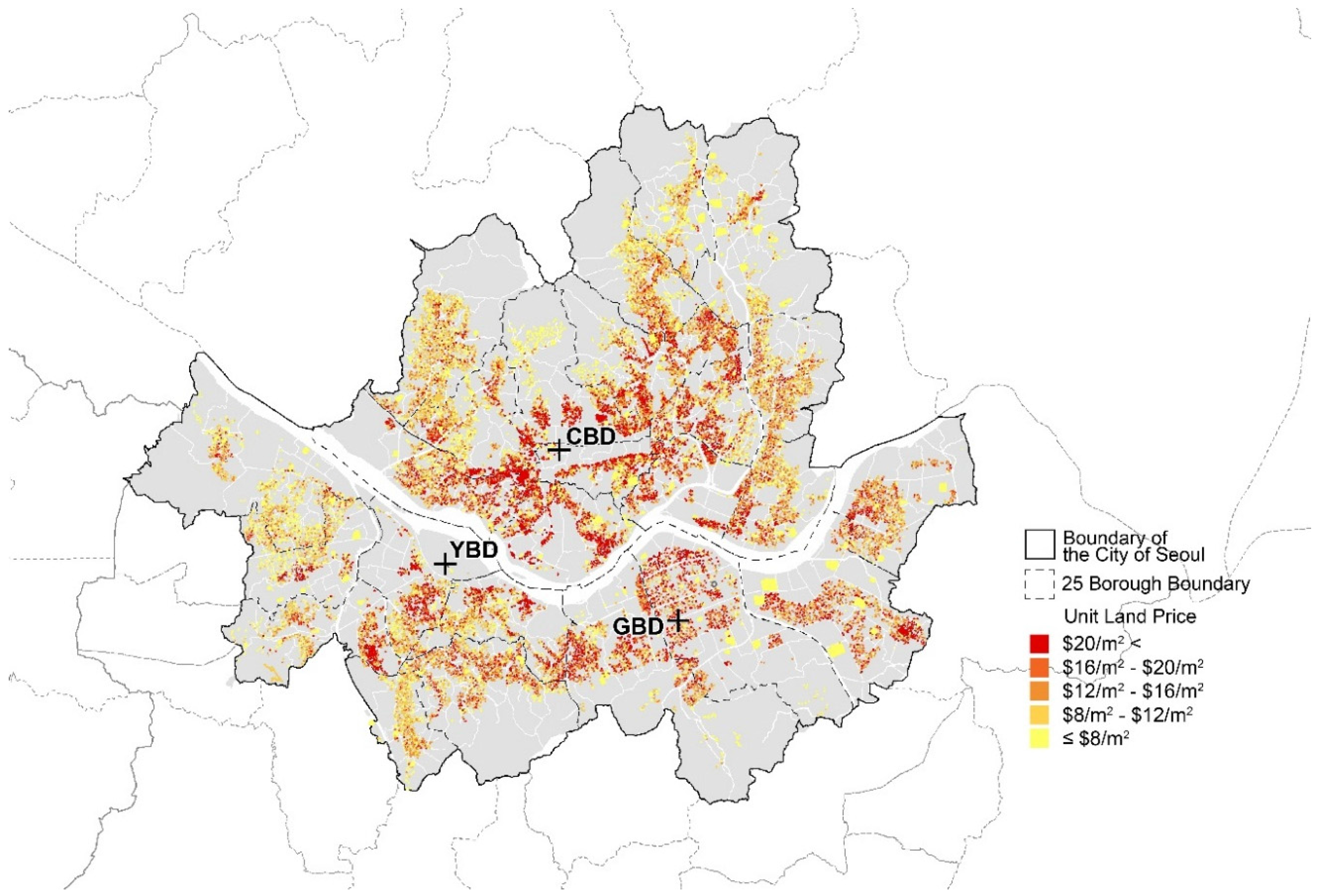
As Seoul has developed apace, three major business submarkets have been established: The Central Business District (CBD), the Gangnam Business District (GBD), and the Yeouido Business District (YBD) [17,18,19]. Among the three, CBD still remains the principal business hub with 30.3% of the total office area in Seoul. GBD follows closely, garnering 25.1%. In terms of office-space inventory, YBD has the lowest market share with 14.6%. The remaining 30% is comprised of local or borough level employment spaces. Figure 1 shows twenty-five boroughs with the three employment centers in Seoul.

3.2. Dataset

This study is based on two different primary datasets. The first one contains micro land value data, which were acquired through a petition to the Administrative Information Request System. Each year the Korea Appraisal Board maintains the price lists of officially selected land parcels for the purposes of taxation or collateral assessment. It is commonly known that the appraised land values are less than the market land values although assessors ascribe values to each parcel according to the most probable selling price in an ordinary market based primarily on the market comparison method [20]. However, since we focus on the marginal value of incremental commercial activities, there is no reason to believe that this appraised value is biased.

Second, we used census block-level demographic and industry data, which are surveyed every five years and distributed through the Statistical Geographic Information System (SGIS). This unit, whose boundary extends to include approximately 500 residents, offers the most fine-grained spatial information about the number of household members and the number of employees in each industry. 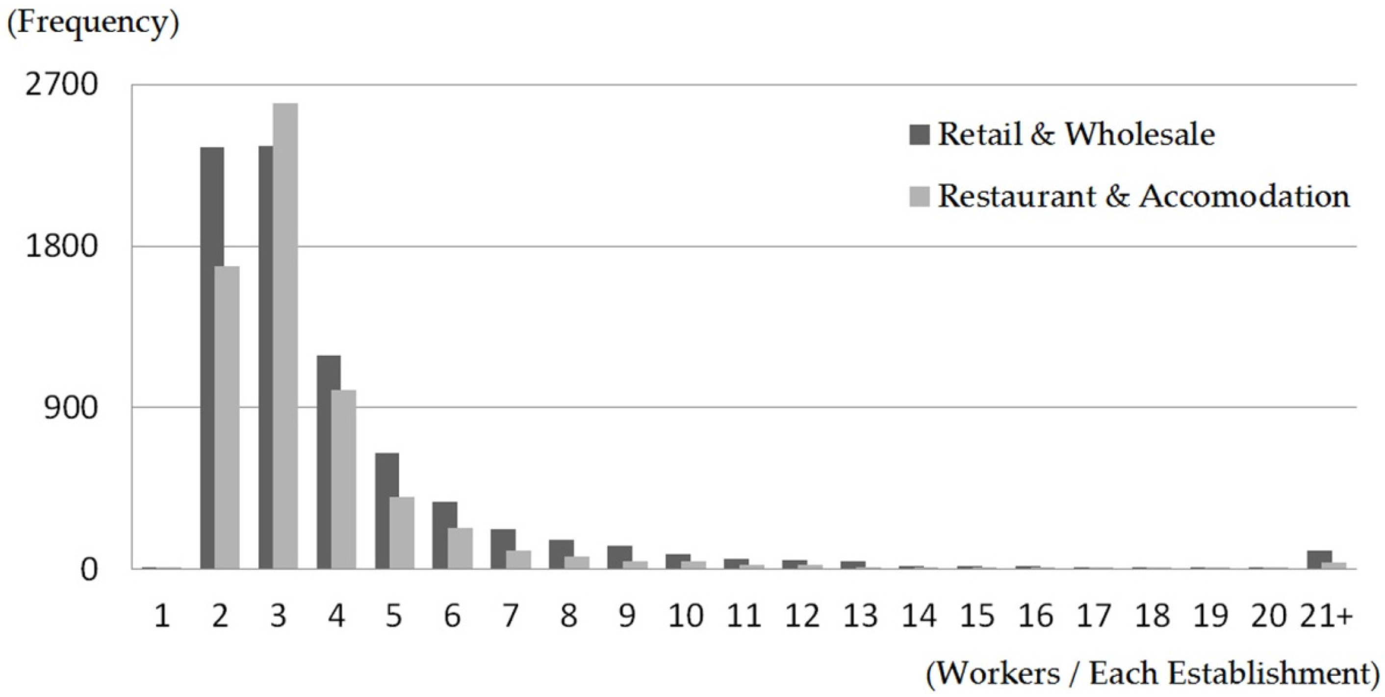The latest SGIS employment data, which were gathered in 2010, provide numbers grouped by the first-level of the 9th Korean Standard Industrial Classification (Appendix A1). Among 21 categories of industry, we combined the numbers of employees in two representative commercial sectors, retail/wholesale business and restaurant/accommodation business. Figure 2 shows the distribution of businesses measured by the number of workers per each establishment. On average, 3.91 workers are in the retail/wholesale business and 3.44 workers are in the restaurant/accommodation business. The variation is much larger in the restaurant/accommodation industry with a maximum of 476 workers, compared to the retail/wholesale industry, which has a maximum of 139 workers.

All data sets are for the 2010 year. The original micro land value data were distributed with the currency of Korean Won and converted with the exchange rate of 1000 Korean Won to 0.92 US Dollar. The officially selected sample parcels included in the area of Seoul originally numbered 30,732. After excluding non-residential parcels and non-urban parcels, the final data set includes 25,126 parcels. As shown in Figure 1, the residential land values range from $0.02/m² to $640.66/m², which yields an average unit land value of $16.45/m².

4. Model Specification

4.1. Methodology

Hedonic price models are utilized to empirically investigate whether proximity benefits related to adjacent commercial activities are offset by disamenity effects. Since land value reflects a parcel’s own characteristics and its spatial attributes regarding other established land uses, the factors that determine residential land value can be summarized as follows:

$$P_i=P\left(N_i, {\mathit{A}}_{\mathit{i}}, {\mathit{L}}_{\mathit{i}}\right)$$

where P_i is the residential land price per unit area of parcel i; N_i indicates nearby commercial activities; A_i and L_i are control variables related to parcel and locational attributes. The vector of a parcel’s own attributes (A_i) constitutes parcel size (A1_i) and imposed zoning ordinance (A2_i). The vector of locational attributes (L_i) measures the accessibility of a parcel i in a macro or micro urban settlement context, which includes employment opportunity at both a city-wide (L1_i) and local level (L2_i) as well as accessibility to public transportation (L3_i) and public facilities (L4_i).

At the neighborhood level of research, geographical scale matters because neighborhood attributes are quantified in a spatially defined area [8]. Thus, we measure the adjacent commercial intensity (N_i) using four different neighborhood scales. The conflicting effects of proximity and disamenity can be compared using quadratic terms [21]. The empirical residential land value function is specified as follows:

$$P_i= {\beta }_0+{\beta }_1{N}_i+{\beta }_2{N}_i{}^2+ {\mathbf{\beta }}_{\mathbf{3}}{\mathit{A}}_{\mathit{i}}+ {\mathbf{\beta }}_{\mathbf{4}}{\mathit{L}}_{\mathit{i}}+{\epsilon }_i$$

4.2. Land Value Determinants

4.2.1. Parcel Attributes

The link between residential land value and parcel size has long been of interest to the field of real estate [22]. Brownstone and De Vany (1991) [23] explain that residential land value is a concave function of parcel size due to subdivision costs. Thorsnes and McMillen (1998) [22] provide empirical support for the concave land value function. However, Colwell and Sirmans (1993) [24] argue that the relationship can be either convex, in relation to land-assembly costs, or concave, in relation to land-subdivision costs.

According to previous research, unit land values have linear relationships to parcel sizes as total land values show concavity or convexity. However, we include the scale variable as a quadratic term by assuming that there is a gain of land assembly above a certain size. The Korean housing market is characterized by high supply and demand for apartment complexes, which are built on large parcels with a greater variety of services and amenities.

Each residential parcel correlates with one zoning ordinance (Appendix A2). These zones are assigned legally permitted maximum FARs (Floor Area Ratios), which are used as a base to decide the final FAR allowed for the future development of a given parcel. The study by Lee and Chung (2004) [25] provided empirical evidence of the effect of additionally achievable density on land values by showing that the two variables have a positive relation. Since achievable density of a parcel is bound by the FAR guidelines of the zone where the parcel exists, we include a zoning dummy variable as a proxy measure for future development potential, which is expected to be an important factor affecting values of residential parcels (

Table 1. Parcels by Residential Zones.

Zoning Ordinance		Maximum FAR (%)	Frequency (N)	Percent (%)	Unit Land Price ($/m2)
Exclusive Residential Zone		100	335	1.33	6.29
General Residential Zone	Type 1	200	2012	8.01	13.02
	Type 2	250	16,000	63.68	16.08
	Type 3	300	5124	20.39	18.46
Quasi-Residential Zone		500	1655	6.59	25.73
Total			25,126	100.00	16.82

).

4.2.2. Location and Accessibility

Land prices are theoretically assumed to decrease with further distance from the urban center and this has been supported by numerous empirical studies [20,26,27]. Using GIS spatial join techniques, we measure job accessibility both city-wide and at the local-level. First, Euclidean distances to the three major business districts, CBD, GBD, and YBD, are measured from 25,126 residential parcels. Those three districts have been conventionally and empirically recognized as major urban centers since Choi’s pioneering study on the Seoul office market (1995) [17]. Second, in order to measure local-level employment opportunities, we set a 3 km buffer in consideration of the average borough size in Seoul. The jobs-housing ratio was calculated with the total number of households divided by the total number of employees in all industries within a 3 km buffer from each residential parcel [28]. As the analysis covers the city area and commuting data per person living on each residential parcel is not available, this variable supplements local-level job accessibility.

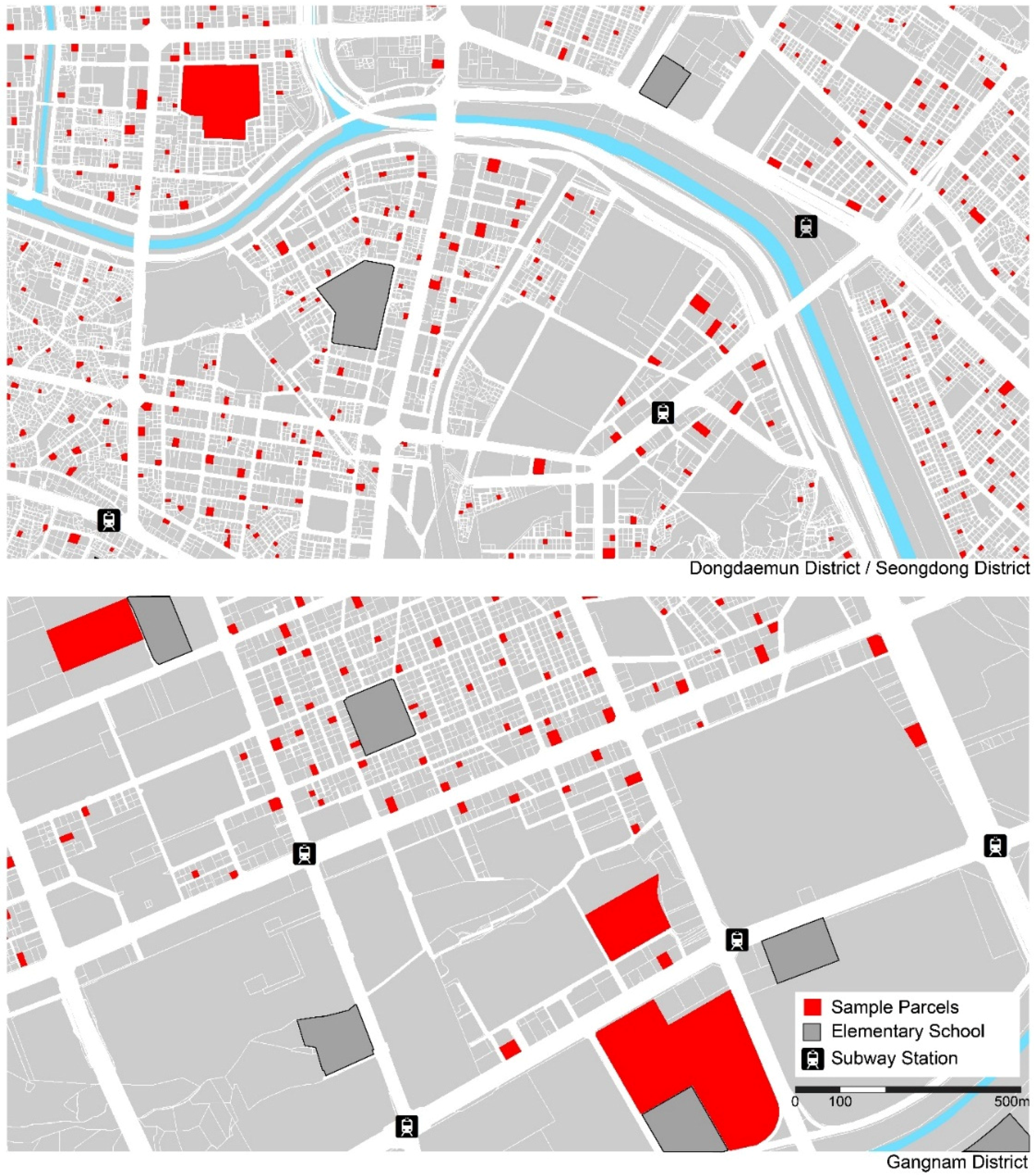
In order to account for more walkable and vibrant residential environments, we include two variables: The distance to the nearest subway station and the distance to the nearest elementary school (Figure 3). Along with public transportation accessibility, proximity to an elementary school is an important factor in choosing the location of a house and therefore greatly affects residential property values in Seoul, a city where most elementary students walk to school by themselves [29,30,31]. To capture how accessible it is by car, we measure the distance to the closest main road from each parcel. In this analysis, main roads are operationally defined to be wider than 12 meters with consideration of the Korean road classification: Primary road (over 40 m), Secondary road (25 m–40 m), Tertiary road (12 m–25 m), Minor or Residential road (below 12 m).

4.2.3. Neighborhood Land Use Attributes

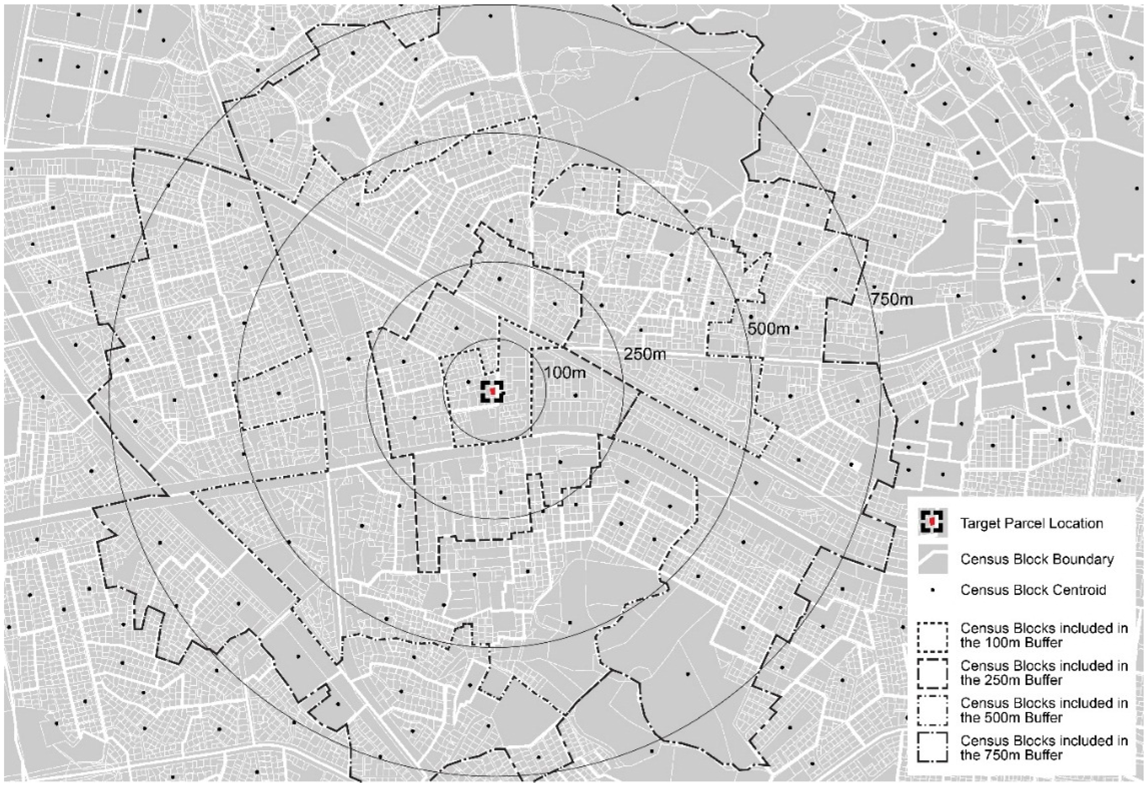
The spatial analysis tool of GIS enables us to join two layers; one is a residential parcel layer holding the price information, and the other is a census-block layer that has commercial employment data in sectors of retail, wholesale, restaurant and accommodation businesses. In order to calculate the total number of employees in commercial sectors surrounding residential areas, we create centroids of polygons for residential parcels and census blocks and subsequently count the census-block centroids falling within each buffer drawn from the residential centroids.

Buffers with 100 m, 250 m, 500 m and 750 m radii are considered to determine the spatial concentration of commercial land use in a neighborhood. A 500 m buffer, which is about one-quarter mile, has been used as an appropriate scale to capture the impacts of the local environment on property values [14,27]. Buffers measuring 250 m and 750 m were introduced simply by multiplication of 500 m. To test effects at a more micro-scale level, a 100 m buffer was also added (Figure 4).

Table 2. Descriptive Statistics.

Variables		N	Mean	Std. Dev.	Min	Max
Price & Size	Unit Land Price ($/m2)	25,126	16.45	14.84	0.02	640.66
	Parcel Area (m2)	25,126	429.17	3677.54	7.60	237,830.70
Neighborhood Attributes	Commercial Emp_100 m	25,126	103.18	207.84	0.00	4621.00
	Commercial Emp_250 m	25,126	585.98	680.68	0.00	13,333.00
	Commercial Emp_500 m	25,126	2264.73	2196.29	0.00	26,067.00
	Commercial Emp_750 m	25,126	5018.72	4754.55	0.00	46,065.00
Location Attributes	Distance_CBD (km)	25,126	8.29	3.70	0.19	17.92
	Distance_GBD (km)	25,126	10.69	4.30	0.19	22.97
	Distance_YBD (km)	25,126	10.06	4.98	0.25	22.84
	Job-Housing Ratio	25,126	1.35	1.09	0.34	6.25
	Nearest Subway (m)	25,126	601.56	415.46	7.28	3921.82
	Nearest Elementary (m)	25,126	335.68	202.98	5.38	2301.05
	Distance_Main Roads (m)	25,126	68.28	72.13	1.00	677.77

summarizes the basic statistics of the variables included in the empirical model. As the location attributes and the neighborhood attributes are measured from the location of each residential parcel, all variables have the same numbers of the residential land parcels, 25,126. The number of commercial employees represents the intensity of commercial activity adjacent to a residential parcel. For the 100 m, 250 m, 500 m, and 750 m buffers, the average numbers of commercial employees are about 103, 586, 2265, and 5019, respectively, showing the expected increase of values according to the size of the neighborhood scales.

4.3. Box-Cox Transformation

To estimate the hedonic price model, we applied the functional form using Box-Cox transformation. The transformed model is:

$$P_i{}^{\left(\theta \right)}= {\beta }_0+{\beta }_1{N}_i+{\beta }_2{N}_i{}^2+\dots + {\gamma }_1{X}_{1i}{}^{\left(\lambda \right)}+{\gamma }_2{X}_{2i}{}^{\left(\lambda \right)}+ {{\displaystyle \sum }}^{\text{}}{\gamma }_j{X}_{ji}+{\epsilon }_i$$

$$where X_i{}^{\left(\lambda \right)}= \{ \begin{array}{c}\frac{ X_i{}^{\left(\lambda \right)}-1}{\lambda } \left(\lambda \ne 0\right) \\ \text{ln} X_i \left(\lambda =0\right)\end{array}$$

As the Box-Cox transformation is suitable to use for positive continuous variables, we investigated the specification of the functional forms for the dependent variable: Residential Land Price, and seven independent variables: Distance to CBD, Distance to GBD, Distancd to YBD, Job-Hosing Ratio, Nearest Subway, Nearest Elementary, and Distance to Main Road. The remaining variables are utilized in linear form.

The maximum likelihood estimates of the transform parameters are $\mathsf{\theta }=0.068, \mathsf{\lambda }=0.351$, while linear ($\mathsf{\theta }=1, \mathsf{\lambda }=1$), multiplicative inverse ($\mathsf{\theta }=-1, \mathsf{\lambda }=-1$), and log specifications ($\mathsf{\theta }=0, \mathsf{\lambda }=0$) are strongly rejected. After taking into consideration of model fitting performances in Appendix A3 and the possibility of substantive interpretations, the final model employed a semi-logarithmic functional form, where the dependent variable takes a logarithmic form ($\mathsf{\theta }=0)$ and all independent variables take linear forms ($\mathsf{\lambda }=1)$.

5. Empirical Results

This study estimated log-transformed residential land value based on parcels’ own attributes as well as their locational and neighborhood attributes. As reported in

Table 3. Box-Cox Regression Results with Commercial Quadratic Variable.

Ln Land Price ($/m2)		Model (1): 100 m Buffer			Model (2): 250 m Buffer			Model (3): 500 m Buffer			Model (4): 750 m Buffer
Parameter		Estimate	(3)	S.E	Estimate		S.E	Estimate		S.E	Estimate		S.E
Neighborhood Attributes
	Commercial Employment (1)	0.162	***	(0.031)	0.089	***	(0.009)	0.015	***	(0.004)	0.005	**	(0.002)
	Commercial Employment Sq.	−0.039	***	(0.015)	−0.006	***	(0.001)	−0.001	*	(0.000)	−0.000		(0.000)
Parcel
	Size	−0.187	***	(0.002)	−0.186	***	(0.002)	−0.187	***	(0.002)	−0.187	***	(0.002)
	Size Sq.	0.001	***	(0.000)	0.001	***	(0.000)	0.001	***	(0.000)	0.001	***	(0.000)
Zoning Ordinance Dummy (2)
	General–Type 1	0.413	***	(0.034)	0.414	***	(0.034)	0.412	***	(0.034)	0.410	***	(0.034)
	General–Type 2	0.701	***	(0.033)	0.692	***	(0.033)	0.695	***	(0.033)	0.697	***	(0.033)
	General–Type 3	0.739	***	(0.034)	0.722	***	(0.034)	0.733	***	(0.034)	0.737	***	(0.034)
	Quasi−Residential	0.922	***	(0.036)	0.898	***	(0.036)	0.921	***	(0.036)	0.928	***	(0.036)
Location & Accessibility
	Distance to CBD	−0.170	***	(0.012)	−0.180	***	(0.012)	−0.173	***	(0.012)	−0.170	***	(0.012)
	Distance to GBD	−0.234	***	(0.010)	−0.221	***	(0.010)	−0.229	***	(0.010)	−0.232	***	(0.010)
	Distance to YBD	0.003		(0.008)	0.003		(0.008)	0.004		(0.008)	0.004		(0.008)
	Job-Housing Ratio	0.081	***	(0.004)	0.074	***	(0.004)	0.077	***	(0.005)	0.078	***	(0.005)
	Nearest Subway	−0.226	***	(0.010)	−0.213	***	(0.010)	−0.220	***	(0.010)	−0.224	***	(0.010)
	Nearest Elementary	−0.138	***	(0.018)	−0.148	***	(0.018)	−0.141	***	(0.018)	−0.137	***	(0.018)
	Distance to Main roads	−0.561	***	(0.054)	−0.541	***	(0.054)	−0.580	***	(0.054)	−0.587	***	(0.054)
Constant		2.451	***	(0.041)	2.425	***	(0.041)	2.440	***	(0.042)	2.447	***	(0.042)
N		25126			25126			25126			25126
R-sq		0.4384			0.4400			0.4382			0.4379
Adj. R-sq		0.4381			0.4397			0.4378			0.4375

Note: Standard error (S.E.) in parentheses; ***, **, * denote significance at the 1, 5, 10 percent levels, respectively. (1) Measurement of commercial employment varies within each model with a different spatial boundary: 100 m, 250 m, 500 m, and 750 m radii from individual residential parcels; (2) The Exclusive Residential Zone is used as a reference category; (3) To make the coefficients easily interpretable, different units from Table 2 are used in the estimation models. Commercial employment: 1000 people; Parcel size: 1000 m²; Nearest subway, Nearest elementary school, and Distance to main roads: 1 km; Distance variables to CBD, GBD, and YBD: 10 km.

, the quadratic term of the commercial variable is included to gauge the conflicting externality effects of nearby commercial activities. In each model, the commercial employment variable is assigned different numerical values in relation to neighborhood scales: A 100 m buffer is used in Model (1); a 250 m buffer in Model (2); a 500 m buffer in Model (3); and a 750 m buffer in Model (4). The adjusted R-squared for the four scales shows 0.438, 0.440, 0.438, and 0.438, respectively.

5.1. Spatial Concentration Effects of Commercial Activities

In Model (1), the single term of the adjacent commercial employment variable exhibits a positive sign, which suggests that residents may value proximity to retail shops or commercial facilities, thus corroborating previous studies [1,13]. Meanwhile, its quadratic term shows a negative sign. This indicates that nearby commercial activities may initially relate to greater residential land values but eventually affect residential environments negatively due to associated disamenities, such as congestion, noise, and litter [11]. The concave curvilinear relationship indicated by the opposite signs suggests a trade-off between the proximity effect and the disamenity effect resulting from adjacent commercial activities.

From Model (1) to Model (4), the magnitudes of the coefficients for both commercial variables decrease, as do the levels of statistical significance. A decline in those figures indicates that the trade-off concerning the positive and negative externalities becomes more difficult to explore as neighborhood scale increases. Further, insignificance of the quadratic term in Model (3) and Model (4) suggests that the 500 m spatial area is too large to capture the impact of the disamenity effects. Following previous studies [1,3], the disamenity effects remain significant within relatively smaller neighborhood scales.

Due to this trade-off relationship, the net benefit of the concentration of commercial activity starts to decrease at a certain point. Each quadratic result indicates that there is a threshold level of mixed land use where the residential land value maximizes in relation to both the proximity effects and the disamenity effects. In terms of commercial employees in a residential neighborhood, threshold levels are 2077 in the 100 m-radius neighborhood scale and 7417 in the 250 m-radius neighborhood scale. As aforementioned, we are unable to recognize the trade-off beyond the 500 m-radius neighborhood-scale analysis.

5.2. Estimation Results of Control Variables

All control variables across the models showed consistent estimation results with the same significance level. First, parcel size shows a convex relationship. Unit land prices initially decrease with greater parcel size because subdivision costs get larger when developers put in sidewalks, sewers, and utility lines. However, as parcels grow beyond a certain level, the unit land price begins to increase. This phenomenon can be explained by the fact that consumers are willing to pay more for large-scale apartment complexes that are affluent in public facilities; thus, large parcels have premium values.

A zoning dummy variable as a proxy for a potential development capacity is statistically significant with the expected positive signs. In our model, the Exclusive Residential Zone is used as a reference category, and other zones appear as binary variables according to the ascending order of their maximum FARs explained in Table 1. Compared to the Exclusive Residential Zone, a parcel in the first type of general residential zone allowing 100% more FAR has approximately 51.1% higher value per square meter, and land in the quasi-residential zone, allowing 400% more FAR, has approximately 151.4% higher value per square meter in case of Model (1). Similar proportional changes are also found in other models.

Consistent with classical location theory, closeness to the business districts CBD and GBD significantly raises land value, but distance to YBD does not have any significant effect in our analysis. This may be explained by the relatively small employment power of the district. The job-housing ratio, looking at local-level job opportunities, has a significantly positive effect on residential land value. Concerning the role of public transportation in land valuation, the distance to the nearest subway variable showed a statistically significant negative sign. In addition, both being near an elementary school and being near a main road raise residential land values by capturing the premium effect.

6. Discussion

In spite of the counter externalities regarding commercial land use, few studies have dealt with impacts of the spatial intensity of commercial activities on residential property values. We have developed an approach that considers not only distance to commercial facilities but also the intensity of commercial activities. By incorporating commercial employment data, we have measured the degree of spatial concentration of commercial properties around each residential parcel and empirically estimated the external effects of commercial land use on residential land values in four neighborhoods, each with a different geographic scale.

As we measured the commercial variable by the number of employees, the threshold levels of adjacent commercial activities are calculated based on the estimates in Table 3.

Table 4. Comparison between Current and Estimated Commercial Employee.

Variables		Threshold Number	Current Mean	Current Max
Commercial Employee	100 m	2077	103	4621
	250 m	7417	586	13,333

Note: The threshold levels of commercial employees are calculated by the following formula, – A/(2 * B), where A refers to the estimates of commercial employment and B refers to the quadratic estimates of commercial employment in Table 3.

presents the threshold number of commercial employees from which the disamenity effect exceeds the proximity effect and the residential land value decreases. Based on the previous findings on the relationship between commercial land use and residential property price in high-density cities, it is plausible to expect that the disamenity effect would be dominant in Seoul [11,12]. Yet comparison with the current average number of commercial employees suggests that promoting mixed land use with further commercial development still has the potential to benefit residents on average.

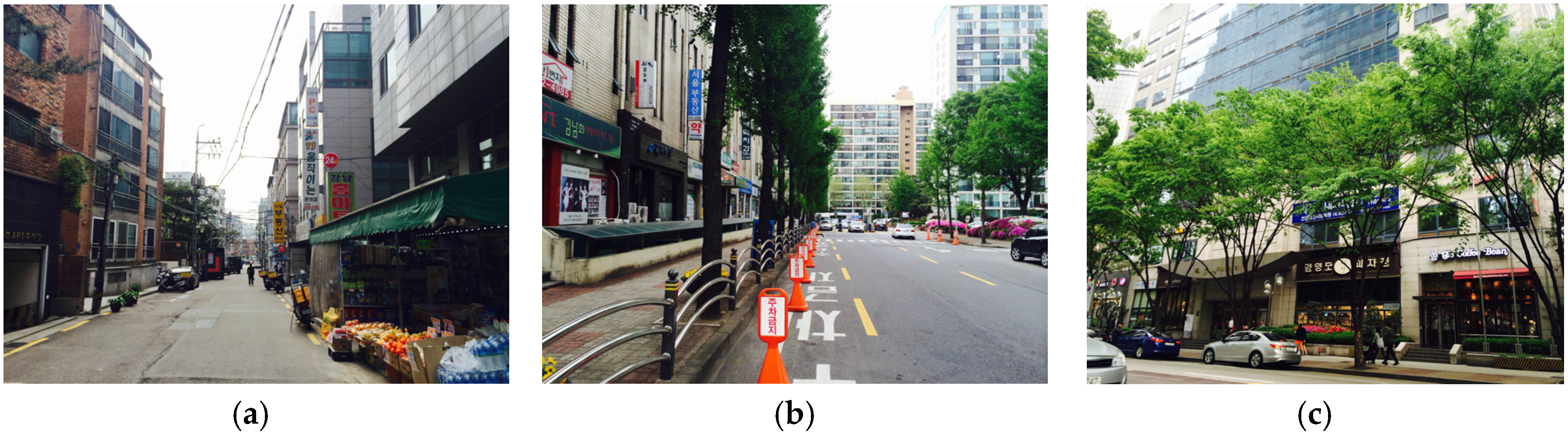
To link our findings to practical implications, we explain several types of commercial developments in residential areas in Seoul. First, we observe a low-to-mid-rise residential area. As zoning code permits, small-scale and neighborhood-serving commercial facilities have closely existed with housing (Figure 5a). In large-scale residential developments, high-rise apartments and separate commercial buildings are developed at the same time. Due to the site design, this type of mixed use tends to be a harmonious arrangement between the residential and commercial area, which is often presented by the inclusion of bicycle, car and pedestrian space. (Figure 5b). Lastly, there is a vertical way of mixing, which often happens in multi-purpose high-rise buildings with high-tech functionality (Figure 5c).

To encourage mixed development in the low-to-mid-rise residential areas, amending the land use zoning system should be taken into consideration. Currently, both ‘Exclusive Residential Zones’ and ‘General Residential Zones’ have strict restrictions through a positive list system, which enumerates in detail what types of uses are permitted. Regulation change from permitting a limited number of uses to restricting a few problematic land uses can enable a more diverse environment. However, there should still be careful investigation of possible problematic and incompatible land uses.

Meanwhile, community-scale design and policy interventions beyond the building level need to be considered to relieve congestion and to better coordinate residential and commercial development. The relatively harmonious mixed-use environment of the high-rise apartment complexes can be attributed to the fact that the complexes are planned and designed in an integrated manner beyond the building level. Similarly, concerted efforts such as street design improvement and planting for noise reduction at the community level may mitigate unpleasant experiences and make places more attractive to residents in other types of mixed-use environments.

7. Conclusions

While taking into account the spatial concentration of employment, this paper verified the trade-off relationship between the proximity effect and the disamenity effect, which expands the views of Li and Brown (1980) [1] and Matthews and Turnbull (2007) [3]. Our quadratic estimation, using Box-cox regression models, showed that increasing commercial activity around residences is related to higher residential land values to some extent, but beyond a threshold level, land values decrease because convenience is offset by excessive congestion or noise.

The trade-off, or the disamenity effect, is appropriate to be measured in small spatial scales. In our analysis, both the magnitude and significance of the coefficients of the commercial variables decrease as the neighborhood scale increases; eventually, the trade-off relationship disappears over the range of a 500 m scale. In addition, a model measured in a 250 m buffer yields slightly more explanatory power than the others.

Our new methodological approach points out the existence of a threshold level with the trade-off relationship. From the calculation of the threshold levels of commercial employees around residences, we suggest mixed land use with further commercial development through a flexible zoning system and community-scale design guidelines. This is in line with the contention of new urbanists. Further studies are necessary regarding specific planning and design methods to achieve a mixed-use environment with less negative externality. Since design features can vary widely with a similar level of spatial intensity of commercial activities, qualitative investigations on mixed-use development will complement this study and help to reach more persuasive solutions in the future.

Careful interpretation of the results will be required. When the location of commercial businesses is chosen based chiefly on vicinity to wealthy neighborhoods, this cross-sectional analysis might be compromised by reverse causality. This paper is less concerned with the possibility of where new commercial developments are established than addressing how residential prices are related to adjacent commercial activities. Also, due to data constraints, the analysis uses the aggregated number of commercial employees in retail, wholesale, restaurant, and accommodation business sectors based on census block level data. Future research needs to consider the contracting externalities of individual sectors of commercial businesses because a single regional shopping center and many stand-alone retail stores might have different impacts on neighborhood environments.

References

- Li, M.M.; Brown, H.J. Micro-neighborhood externalities and hedonic housing prices. Land Econ. 1980, 56, 125–141. [Google Scholar] [CrossRef]
- Pivo, G.; Fisher, J.D. The walkability premium in commercial real estate investments. Real Estate Econ. 2011, 39, 185–219. [Google Scholar] [CrossRef]
- Matthews, J.W.; Turnbull, G.K. Neighborhood street layout and property value: The interaction of accessibility and land use mix. J. Real Estate Financ. 2007, 35, 111–141. [Google Scholar] [CrossRef]
- Platt, R.H. Land Use Control: Geography, Law, and Public Policy; Presidence Hall: Englewood Cliffs, NJ, USA, 1991; pp. 179–181. [Google Scholar]
- Fischel, W. An economic history of zoning and a cure for its exclusionary effects. Urban. Stud. 2004, 41, 317–340. [Google Scholar] [CrossRef]
- Fischel, W. The Economics of Zoning Laws; The Johns Hopkins University Press: Baltimore, MD, USA, 1985; pp. 231–251. [Google Scholar]
- Cervero, R.; Kockelman, K. Travel demand and the 3ds: Density, diversity, and design. Transp. Res. D 1997, 2, 199–219. [Google Scholar] [CrossRef]
- Duncan, M.J.; Winkler, E.; Sugiyama, T.; Cerin, E.; Dutoit, L.; Leslie, E.; Owen, N. Relationships of land use mix with walking for transport: Do land uses and geographical scale matter? J. Urban Health 2010, 87, 782–795. [Google Scholar] [CrossRef] [PubMed]
- Ewing, R.; Cervero, R. Travel and the built environment: A synthesis. Transp. Res. Rec. 2001, 1780, 87–114. [Google Scholar] [CrossRef]
- Song, Y.; Knaap, G.J. Measuring the effects of mixed land uses on housing values. Reg. Sci. Urban Econ. 2004, 34, 663–680. [Google Scholar] [CrossRef]
- Mahan, B.L.; Polasky, S.; Adams, R.M. Valuing urban wetlands: A property price approach. Land Econ. 2000, 76, 100–113. [Google Scholar] [CrossRef]
- Frew, J.; Jud, G.D. Estimating the value of apartment buildings. J. Real Estate Res. 2003, 25, 77–86. [Google Scholar]
- Cervero, R.; Duncan, M. Neighbourhood composition and residential land prices: Does exclusion raise or lower values? Urban Stud. 2004, 41, 299–315. [Google Scholar] [CrossRef]
- Koster, H.R.A.; Rouwendal, J. The impact of mixed land use on residential property values. J. Reg. Sci. 2012, 52, 733–761. [Google Scholar] [CrossRef]
- Sung, H.; Oh, J.T. Transit-oriented development in a high-density city: Identifying its association with transit ridership in Seoul, Korea. Cities 2011, 28, 70–82. [Google Scholar] [CrossRef]
- Thorsnes, P. Internalizing neighborhood externalities: The effect of subdivision size and zoning on residential lot prices. J. Urban Econ. 2000, 48, 397–418. [Google Scholar] [CrossRef]
- Choi, M.J. The Seoul office market: Characteristics, trend, and prospect. J. Korean Plan Assoc. 1995, 30, 143–159. [Google Scholar]
- Kim, H.M.; Han, S.S. Seoul. Cities 2012, 29, 142–154. [Google Scholar] [CrossRef]
- Cushman and Wakefield. Cushman and Wakefield Quarterly Report Q3, 2012; MARKETBEAT Office Snapshot: Seoul, South Korea, 2012. [Google Scholar]
- Choi, M.J. Spatial and Temporal Variations in Land Values: A Descriptive and Behavioral Analysis of The Seoul Metropolitan Area. Ph.D. Thesis, Harvard University, Cambridge, MA, USA, 1993. [Google Scholar]
- Gujarati, D.; Porter, D. Basic Econometrics; McGraw Hill: New York, NY, USA, 2009; pp. 210–213. [Google Scholar]
- Thorsnes, P.; McMillen, D.P. Land value and parcel size: A semi-parametric analysis. J. Real Estate Financ. 1998, 17, 233–244. [Google Scholar] [CrossRef]
- Brownstone, D.; Devay, A. Zoning, returns to scale, and the value of undeveloped land. Rev. Econ. Stat. 1991, 73, 699–704. [Google Scholar] [CrossRef]
- Colwell, P.F.; Sirmans, C.F. A comment on zoning, returns to scale, and the value of undeveloped land. Rev. Econ. Stat. 1993, 75, 783–786. [Google Scholar] [CrossRef]
- Lee, C.M.; Chung, E.C. The effect of density potential on land value in urban redevelopment: The case of residential areas in Seoul. J. Korean Plan Assoc. 2004, 39, 117–130. [Google Scholar]
- Kau, J.B.; Sirmans, C.F. Urban land value functions and the price elasticity of demand for housing. J. Urban Econ. 1979, 6, 112–121. [Google Scholar] [CrossRef]
- McMillen, D.P. Consistent estimation of the urban land value function. J. Urban Econ. 1990, 27, 285–293. [Google Scholar] [CrossRef]
- Peng, Z.R. The jobs-housing balance and urban commuting. Urban Stud. 1997, 34, 1215–1235. [Google Scholar] [CrossRef]
- Kim, S.N.; Ahn, K.H. Examining the children’s mode choice for the school trip and its determinants: A morphological case study on the elementary school neighborhoods in Seoul. J. Urban Des. Inst. Korea 2010, 11, 93–112. [Google Scholar]
- McDonald, N.C.; Aalborg, A.E. Why Parents Drive Children to School: Implications for Safe Routes to School Programs. J. Am. Plan. Assoc. 2009, 75, 331–342. [Google Scholar] [CrossRef]
- Schlossberg, M.; Greene, J.; Phillps, P.P.; Johnson, B.; Parker, B. School trips: Effects of urban form and distance on travel mode. J. Am. Plan. Assoc. 2006, 72, 337–346. [Google Scholar] [CrossRef]
© 2016 by the authors; licensee MDPI, Basel, Switzerland. This article is an open access article distributed under the terms and conditions of the Creative Commons Attribution (CC-BY) license (http://creativecommons.org/licenses/by/4.0/).