
The Impact of Urbanization on Energy Intensity in Saudi Arabia


1
Laboratoire du Management d’Innovation et du Développement Durable, Université de Sousse, Sousse 4023, Tunisia
2
College of Administrative Sciences, Najran University, Najran 1988, Saudi Arabia
*
Author to whom correspondence should be addressed.
†
These authors contributed equally to this work.
Sustainability 2016, 8(4), 375; https://doi.org/10.3390/su8040375
Submission received: 25 February 2016
/
Revised: 9 April 2016
/
Accepted: 12 April 2016
/
Published: 16 April 2016
(This article belongs to the Section Sustainable Urban and Rural Development)
Abstract
:This paper investigates the long-term and causal relationship between energy intensity, real GDP per capita, urbanization and industrialization in Saudi Arabia over the period 1971–2012 using the breakpoint unit root tests developed by Perron (1989) and the autoregressive distributed lag (ARDL) model bounds testing to cointegration proposed by Pesaran et al. (2001) and employing a modified version of the Granger causality test proposed by Toda and Yamamoto (1995). Additionally, to test the robustness of the results, the fully modified ordinary least squares (OLS) regression, the dynamic OLS regression, and the Hansen test are used. Our results show that the variables are cointegrated when energy intensity is the dependent variable. It is also found that urbanization positively affects energy intensity in both the short term and the long term. Causality tests indicate that urbanization causes economic output that causes energy intensity in the long term. Our results do not support the urban compaction hypothesis where urban cities benefit from basic public services and economies of scale for public infrastructure. Therefore, measures that slow down the rapid urbanization process should be taken to reduce energy intensity in Saudi Arabia. In addition, reducing energy inefficiency in energy consumption should be a strategy to attain sustainable development in the near future in Saudi Arabia.
1. Introduction
According to the projections of the United Nations, urban cities will absorb a projected 2.3 billion global population growth over the next 40 years; thus, the importance of that phenomenon has led various empirical studies to model urbanization as one of the driving factors of energy consumption [1]. In energy economic literature, there are many studies that have investigated the impact of urbanization on energy use at aggregate (e.g., total energy consumption) or disaggregate (e.g., electricity consumption, road transport energy consumption) levels. In general, the findings of various empirical studies are mixed and have not led to a clear conclusion. Some have concluded that urbanization positively affects energy consumption [2,3,4,5,6,7,8,9,10,11]. Others empirical works have found that urbanization can negatively affect energy use [12,13,14,15]. The conflicting empirical results are attributed to many factors such as the data and methodologies used and the non-consideration of differences in the stage of development [13]. The majority of previous empirical works assumed that the effect of urbanization is homogenous for all countries or that it is not true due to the differences in energy structure, development stages and urban infrastructure across countries [13].
However, few empirical studies have investigated the effects of urbanization on energy intensity [16,17]. Generally, energy intensity is measured by energy consumption divided by gross domestic product (GDP). It indicates the degree of dependence of an economy to energy. Investigating how urbanization affects energy intensity in Saudi Arabia may provide additional insights regarding sustainable development in the country. A reduction in energy intensity can play a crucial role in protecting the environment through the reduction of carbon dioxide emissions (CO2) and ensuring energy security.
To our knowledge, our study is the first that examines how urbanization influences energy intensity in Saudi Arabia. Saudi Arabia's energy intensity (energy consumption per unit of GDP) is relatively very high [18]. The overuse of energy is the result of many factors such as the high population growth rate, the rapid urbanization, and energy-intensive industries and lifestyles. The reduction of energy intensity can be a tool to mitigate the impacts of energy on climate change [16].
In general, energy intensity is highly correlated with GDP, and countries with higher GDP have lower energy intensity than countries with lower GDP. In fact, the GDP per capita causes energy use by allowing changes in the demand structure so that energy consumption increases and then decreases as the economy passes from the agricultural-intensive economy to the industrial and then onto the service-intensive economy stage. In the final post-industrial stage, energy intensity decreases because less energy-intensive materials characterize the economy based on the service sector [19,20]. In addition to GDP, some other factors such as urbanization and industrialization may affect energy intensity. Urbanization can affect energy intensity positively or negatively depending on the impact of urbanization on economic activity through a higher concentration of consumption and production, and hence generating more pollutant emissions [4,6,13,21]. In addition, urbanization leads to economies of scale, which provide the opportunity for increases in energy efficiency [12,13]. Finally, it is expected that industrialization has a positive impact on energy intensity.
Comparatively to previous studies, we use a dynamic model, which allows detecting short- and long-term effects. In contrast, static models lead to spurious regression results. Our paper provides novel insights to the urbanization-energy literature by exploring the impact of urbanization on energy intensity in Saudi Arabia. Analyzing how urbanization affects energy intensity is an interesting topic because reducing energy intensity can help mitigate the impacts of climate change through the implementation of policies based on energy efficiency and savings [22]. Income, industrialization, services share in GDP, and urbanization elasticities of energy intensity will be determined in the short and long term.
The implications of the findings for energy policy will be discussed. For example, a negative elasticity of income means that economic policies that increase income in Saudi Arabia will decrease energy intensity. In addition, a positive elasticity of industrialization implies that increases in industrialization will increase energy intensity. Thus, industrial policy aimed at speeding up industrialization will increase energy intensity. A positive urbanization elasticity means that urbanization leads to an increase in energy intensity. Hence, the combined effects of increasing income, industrialization, and urbanization will lead to a fall in energy intensity only if income growth is sufficiently large enough to offset the impact of urbanization and industrialization. Improvements in energy intensity are necessary in Saudi Arabia by taking measures based on energy efficiency, conservation, and the use of advanced technology.
Being the largest economy in the Gulf region, Saudi Arabia is an interesting case study as it faces high energy intensity. Our study aims to contribute to the understandings on the impacts of urbanization on energy intensity, and gain insights for future urbanization policies, and contribute to the development of climate change policies in which urbanization can be taken into account [22].
We organize the rest of the paper as follows. In Section 2, the material and the different methods used are presented. Firstly, we focus on the different channels by which urbanization can positively or negatively affect energy use or intensity. Secondly, we give a brief overview of the situation of urbanization and energy intensity in Saudi Arabia. Thirdly, we provide a brief literature review. Lastly, we present data and models used in this study. In Section 3, we present the empirical results and their discussions. Finally, Section 4 reports conclusions and policy implications.
2. Material and Methods
2.1. Impact of Urbanization, Industrialization, and Income on Energy Use
Many studies have shown that urbanization can affect energy use or energy intensity through several channels [4,16,17,21,23]. First, urban infrastructure needs to consume more energy through the expansion of economic activities. In addition, urbanization leads production to shift from agriculture that is less energy-intensive to manufacturing industries, which are more energy-intensive. Second, modern buildings operate with more energy consumption equipment (e.g., refrigerators and air conditioning). Third, in urbanized cities, there is more motorized traffic and congestion, which leads to more energy use [2,15,16,21,23].
At the same time, technological mechanisms (e.g., energy-saving buildings, efficient home appliances, central heating systems, fuel-efficient transportation, etc.) lead to reduced energy consumption within buildings and transportation in urban cities [17]. In addition, a high population density in urban cities allows for economies of scale in urban public infrastructures through the reduction of private car use and travel distances, and the reduction in losses of electricity supply, thus causing a reduction of energy consumption [17]. In addition, urbanization can afford some economies of scale to decrease energy consumption mainly in public services (e.g., health and primary education), which are equally provided to urban (more populated) and rural regions (less populated). We call this energy-saving effect [4,17].
Globally, the impact of urbanization on energy use or energy intensity can be positive or negative because urbanization leads to the expansion of economic activity through a higher concentration of consumption and production, but it also leads to economies of scale and provides an opportunity for increases in energy efficiency.
Industrialization leads in general to an increase in energy consumption because industrial activities (e.g., petroleum refining, primary metals, chemicals, paper and allied products, and manufacturing) consume more energy than traditional agricultural activities or textile industries [16,21,24]. In addition, the industrialization promotes the urbanization process through the migration of labor force from agricultural regions to the urban manufacturing cities [25].
It is also shown that energy intensity declines as income increases [19]. This is explained by the structural change of the economy from pre-industrialization stages based on agriculture (more energy-intensive) to post-industrialization stages based on services (less energy-intensive), and technological progress leads to increases in energy efficiency and to the usage of substitute materials that are less energy-intensive.
In addition, the increase in income and the technological development have led economic systems to switch from a system based on traditional biomass to a system based on fossil fuels [17]. The rapid urbanization and industrialization in many regions in the world facilitates and accelerates the energy transition, which leads to more energy use and hence more problems of environmental degradation. However, it is unclear whether the influence of urban cities expansion on energy consumption and carbon dioxide emissions varies due to different levels of development of an economy or income [13].
2.2. Urbanisation and Energy Intensity in Saudi Arabia
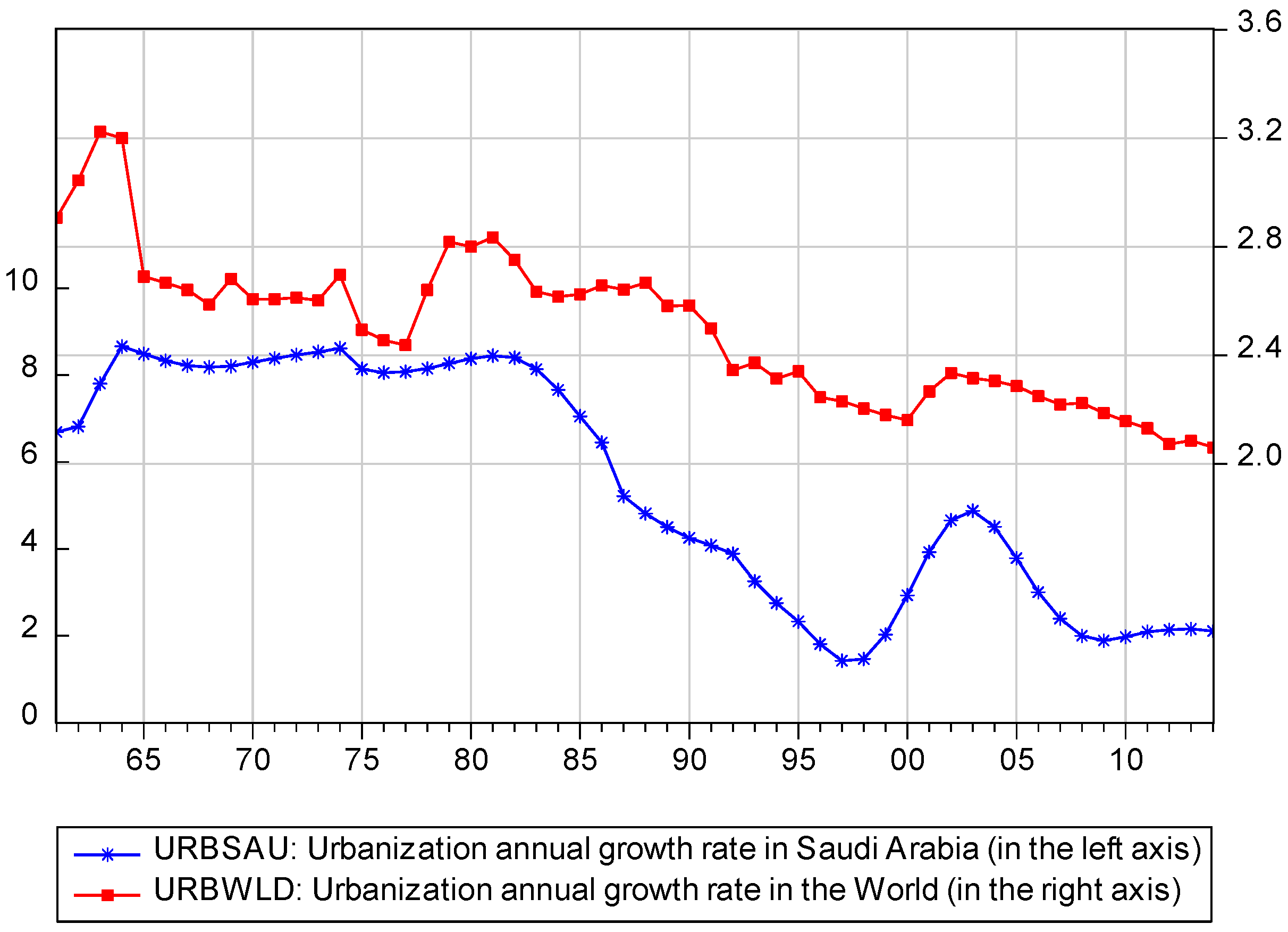
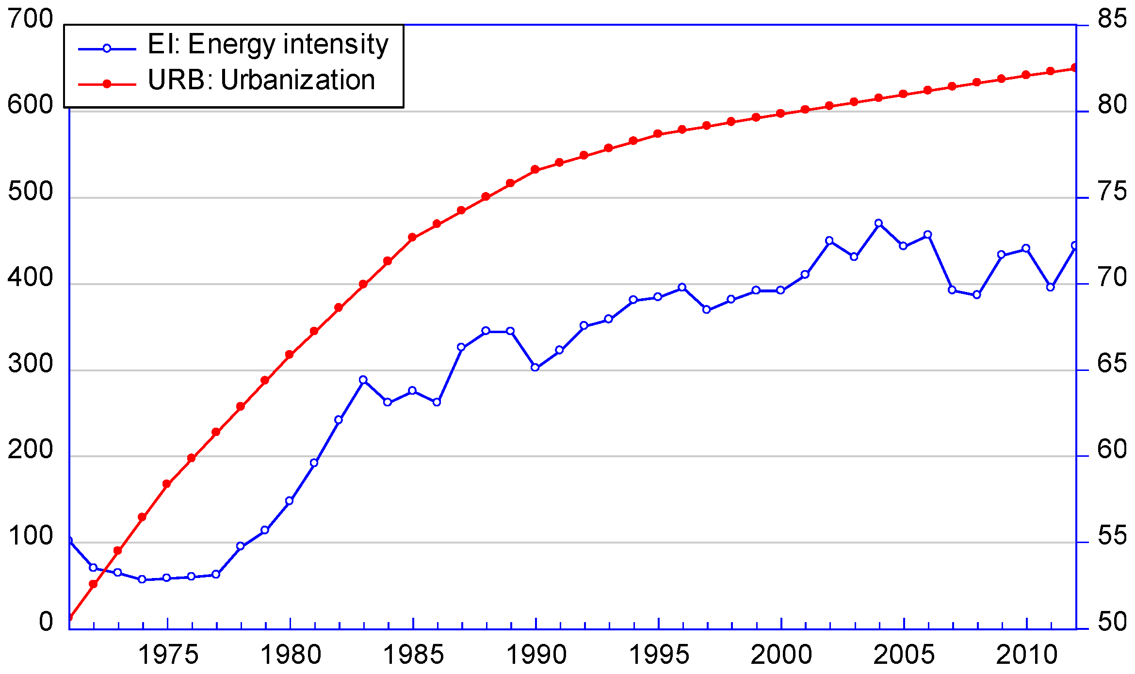
The urbanization rate (part of population living in urban areas) has been increasing in Saudi Arabia since 1960. It reached a rate of 82% in 2010, whereas the worldwide urbanization rate reached only 51.5% in the same year [26]. The Saudi Arabia urban population had increased from 1.272 million in 1960 to 24.354 million in 2014 [26]. The urban population annual growth in Saudi Arabia is very high comparatively to worldwide urban population annual growth (Figure 1). As Saudi Arabia is an abundant oil country, petroleum fuels represent the base for urbanization. The correlation coefficient between urbanization and energy use is about 84% over the period 1971–2012. As shown in Figure 2, the urbanization rate in Saudi Arabia passed from 50.6% in 1971 to 82.5% in 2012. Continuous urbanization may promote Saudi Arabia's economic growth. For the case of energy intensity in Saudi Arabia, it has experienced a decline from 1971 to 1976, a rapid increase from 1976 to 2006 and a steady decline in recent years. It passed from 59.74 in 1976 to 456.24 in 2006 (for more details, see Figure 2). In addition, rapid urbanization in Saudi Arabia may put enormous pressure on the environment.
In consequence, the impact of urbanization on energy intensity in Saudi Arabia is a problematic that should be investigated. Hence, examining how urbanization affects energy intensity in Saudi Arabia can be interesting for policy makers and urban planners.
2.3. Review of Empirical Studies
The impact of urbanization on energy use has been extensively studied in the existing literature. We are limited here to econometric studies. Many previous studies (e.g., [2,3,4,5,6,8,9,10,11,17,27] found that urbanization positively affects energy consumption. Jones [2] analyzed the effect of urbanization on energy use by estimating a regression linear model for 59 developing countries during the year 1980. He found that urbanization positively affects energy consumption, and the urbanization elasticity of energy use varied from 0.35 to 0.48. By using a panel data set of developed and developing countries over the period 1965–1987, Parikh and Shukla [4] found similar results to Jones [2]. Their findings showed that urbanization has a significant and positive impact on energy use; and urbanization elasticity of energy use is in the range of 0.28 to 0.47. By estimating a linear regression model by the ordinary least squares (OLS) method, Burney [3] also found a positive impact of urbanization on electricity consumption per capita using cross-sectional data for the year 1990 for 93 countries. Moreover, by using an error correction model Holtedahl and Joutz [5] found that urbanization positively affects residential energy consumption in Taiwan in both the short term and the long term over the period 1956–1995. They explained their findings by the easy access to electricity in urban cities. By studying a group of advanced European countries and employing the stochastic impacts by regression on population, affluence, and technology (STIPAT) model, York [6] also found a positive impact of urbanization on energy use. His finding showed that urbanization elasticities are in the range of 0.29 to 0.56. By using an econometric time series technique based on the autoregressive distributed lag (ARDL) bounds testing to cointegration approach, Liu [27] found a long-term relationship between energy consumption, GDP, urbanization, and population in China over the period extended from 1978 to 2008. The results of the Granger causality test indicated that urbanization causes energy consumption in both the long term and short term. In addition, by using the factor decomposition model, Liu [27] found that the contribution share of urbanization on energy consumption is positive but is decreasing due to energy efficiencies. Poumanyvong et al. [10] studied the impact of urbanization on road energy consumption for a group of low-, middle-, and high-income countries during the period of 1975 to 2005 by using the STIRPAT model. They found that urbanization has a positive impact on road energy use in all countries, but the magnitude of its influence is greater in high-income countries group than in the other country groups. Shahbaz and Lean [8] studied the causal relationships between urbanization, energy consumption, economic growth, industrialization, and financial development in Tunisia over the period of 1971 to 2008 by employing the ARDL bounds testing to cointegration approach and the Johansen multivariate cointegration approach. They found the existence of long-term relationship among energy consumption, economic growth, financial development, industrialization, and urbanization in Tunisia. In addition, they found that Tunisia’s urbanization positively and significantly affects energy consumption in the long term, whereas its impact is insignificant in the short term. A 1% increase in Tunisia’s urban population leads to an increase of 0.9% in its energy consumption in the long term. Using the same methodology employed by Shahbaz and Lean [8], Adom et al. [9] found a positive impact of urbanization on electricity consumption in Ghana over the period 1975–2005. Al-mulali et al. [11] studied the relationship between energy consumption, urbanization, and CO2 emissions for a panel of the Middle East and North Africa (MENA) countries over the period 1980–2009. They found that the three variables are cointegrated and there is a long-term bi-directional positive relationship between urbanization, energy consumption, and CO2 emissions. The authors suggested that MENA countries should slow the rapid increase in urbanization in order to reduce energy consumption and CO2 emissions in the region. More recently, Ma [17] investigated the impact of urbanization on energy intensity, electricity intensity, and coal intensity in China using dynamic models and panel datasets at the provincial level over the period 1986–2011. The empirical findings revealed that China’s urbanization positively affects energy intensity and electricity intensity in the long term, but it does not influence coal intensity. From these results, the author concluded that energy policies linked to the urbanization process should be province-specific.
On the other hand, some studies found that urbanization negatively influences energy use (e.g., [12,14,28]). For example, by estimating an environmental Kuznets curve (EKC) semi-log model for a group of 23 OECD countries over the period 1960–2000, Liddle [12] found that the impact of urbanization on road energy consumption is negative. Using an OLS regression analysis, Ewing and Rong [28] found that urbanization negatively affects residential energy use in the United States. Using panel data models for 94 countries over the period covering the years from 1981 to 2007, Fang et al. [14] found that the impact of urbanization on total energy consumption is negative for high-income countries but not significant for low-income countries.
Finally, some other studies found mixed results (e.g., [7,13,15,29,30,31]). By using annual series data from 1968 to 2005, Halicioglu [29] studied the relationship between urbanization, residential energy use, energy prices, and GDP for Turkey by estimating dynamic models based on the ARDL bounds testing for cointegration approach. The author found that urbanization Granger causes residential energy use in the long term but not in the short term. Two years after, Mishra et al. [7] studied the relationship between urbanization, GDP, and energy consumption for a group of Pacific Island countries over the period of 1980 to 2005. They found that increases in urbanization lead to increases in energy consumption in the countries of Fiji, French Polynesia, Samoa, and Tonga, whereas urbanization negatively affects energy consumption in New Caledonia.
Poumanyvong and Kaneko [13] investigated the impact of urbanization on energy use and CO2 emissions by estimating a STIPAT model for a sample of 99 countries over the period 1975–2005. Their results revealed that the effect of urbanization on energy use depends on the stages of development (income classes). Urbanization positively affects energy consumption in the countries with middle and high incomes, or it negatively affects energy use in the low-income group. The impact of urbanization on CO2 emissions is positive for all income groups. In addition, the impact of industrialization on energy use is positive in the countries with low and middle incomes. Krey et al. [30] used integrated assessment models to analyze the impact of urbanization on residential energy use in China and India. They found that urbanization does not affect residential energy use directly, but the relationship between urbanization and energy use depends upon how labor productivity affects economic growth. Studying the same countries as Krey et al. [30], O’Neill et al. [31] used a computable general equilibrium model to investigate the impact of urbanization of energy. They found that the direct effect of urbanization on energy consumption is not that strong and much of the impact of urbanization on energy use comes through the impact that an increased labor supply has on economic growth. Wang [15] found that urbanization reduces residential energy use because of the economies of scale and technological advances associated with urbanization, whereas the growth of economic activities caused by the urbanization process leads to an increase in energy consumption in China.
Even though there are many studies investigating the effect of urbanization on energy use, much less has been done on the influence of urbanization on energy intensity (e.g., [16,20,21,24,32]). The pioneering work of Jones [21] was the first that analyzed the impact of income, urbanization, and industrialization on energy intensity in 59 developing countries for the year 1980. He found that the different long-term elasticities of income, urbanization, and industrialization are equal to 0.77, 0.35 and 1.35, respectively. Galli [32] estimated the impact of income on energy intensity in ten Asian countries over the period 1973–1990. The empirical results showed that income negatively affects energy intensity in the long term. Samouilidis and Mitropoulos [24] found long-term elasticities of industrialization to energy intensity in the range of 0.90 to 1.96 and short-term elasticities in the range of 0.17 to 0.46 for the case of Greece. Sadorsky [16] analyzed the impact of income, industrialization, and urbanization on energy intensity for a group of 76 developing countries over the period 1980–2010 by using heterogeneous panel regression techniques. He found negative income elasticities and positive industrialization elasticities of energy intensity, whereas the effect of urbanization is mixed. When considering energy intensity as dependent variable, the impact of income variable reflects only the technique effect and not the scale effect. Elliot et al. [20] studied the influences of urbanization and industrialization on energy intensity in China using a group of 29 provinces over the period 1997–2010. Their findings showed that industrialization is the overwhelming contributor to Chinese energy intensity, with elasticities ranging from 0.62 to 0.66 in the short term and slightly higher in the long term. This confirms that China has experienced industry-led economic development. The rapid expansion of energy-intensive sectors has had a serious effect on other energy sectors.
2.4. Methodology and Data
2.4.1. Breakpoint Unit Root Tests
The major drawback of standard unit root tests such as the augmented Dickey–Fuller (ADF), Phillips–Perron (PP), Elliot, Rothenberg, and Stock (ERS), and Ng and Perron (NP) tests is that they suppose that the deterministic trend is correctly specified. Otherwise, according to Perron [33], they are biased toward a trend stationary with an exogenous structural break null hypothesis, and the conventional unit root tests will conclude the presence of a unit root when in fact it does not exist. This observation has led to the development of breakpoint unit root tests that take into account the structural change in the series [34]. These tests are a modified augmented Dickey-Fuller tests that allow for levels and trends to differ across a break date.
Following Perron [33], Perron and Vogelsang [35,36] and Vogelsang and Perron [37], we present four models of breakpoint unit root tests where the null hypothesis supposes that the series follows a unit root with a possible break against the alternative hypothesis that implies the presence of a trend stationary with a break alternative. For an innovational outlier, they are expressed in the following forms:
Model 0:
Model 1:
Model 2:
Model 3:
where and 0 otherwise; and 0 otherwise; and 0 otherwise; DUt is a dummy variable that captures a break in the intercept; DTt represents a break in the trend occurring at time ; Dt is a one-time break dummy variable; is the break date; is the first difference operator; and is a white noise term.
Model 0 supposes a non-trending series with a break in the intercept (the coefficients β and λ are set equal to 0); Model 1 supposes a trending series with a break in the intercept (the coefficient λ is set equal to 0); Model 2 supposes a trending series with a break in the intercept and trend; and Model 3 supposes a trending series with a break in trend (the coefficients θ and ω are set equal to 0). Since the appropriate model and the optimal lag lengths are crucial in interpreting the results of the tests, we select a breakpoint by minimizing the Dickey-Fuller t-statistic, and selecting the lag length based on the Schwarz information criterion.
2.4.2. The ARDL Bounds Testing to Cointegration Approach
In order to study the effects of urbanization, real GDP per capita, industrialization, and services on energy intensity in Saudi Arabia, we use the model proposed by Jones [21] and extended by Holtedahl and Joutz [5] and Sadorsky [16]. As explained above, this model links the energy intensity (EI) to the real GDP per capita, the urbanization rate (URB), the industrialization share in GDP (IND), and the services share in GDP (SER) as follows:
Taking the natural logarithm form of Equation (5), we obtain:
where L denotes the natural logarithm function; t denotes the years from 1971 to 2012; εt is the error term; β0, β1, β2, β3, and β4 are the parameters to be estimated that reflect, respectively, a constant, income elasticity of energy intensity, urbanization elasticity of energy intensity, industrialization elasticity of energy intensity, and services elasticity of energy intensity.
As some or all of the variables are not stationary in levels but integrated of order one (I(1)), the relationship given in Equation (6) can also be specified as an ARDL model. The ARDL model is a dynamic version of the static model given in Equation (5). It has advantages over static model because it permits the determination of both short- and long-term elasticities of energy intensity for the different independent variables in addition to the correction for the problem of residual serial correlation and endogenous regressors [38,39].
The ARDL bounds testing to cointegration approach of Pesaran and Shin [39] and Pesaran et al. [40] is used to check for existence of a long-term relationship between energy intensity, income, urbanization, industrialization, and services share in GDP in Saudi Arabia. To do so, we estimate the unrestricted error correction model (UECM) as follows:
where and L are, respectively, the first difference order and the natural logarithm that are used in front of variables. The bounds testing consists to test the null hypothesis of no cointegration between the variables in the UECM: H0: δ1 = δ2 = δ3 = δ4 = δ5 = 0. According to Pesaran et al. [40], we reject the null hypothesis of no cointegration if the computed joint F-statistic is superior to the two critical bounds values for a given significance level of 1%, 5%, or 10%. Otherwise, the variables are not cointegrated when the F-statistic is inferior to the lowest critical bounds value, and we cannot conclude when the F-statistic lies between the two critical bounds values. We compute the lowest critical bounds value when all the variables are integrated of order zero, whereas the upper critical bounds value is computed when all the variables are integrated of order one. Pesaran et al. [40] and Narayan [41] provided the two critical bounds values.
If we find that the variables are not cointegrated, we estimate the model given in Equation (6) using the first difference for the variables integrated of order one. However, if the variables investigated are cointegrated, we estimate an error correction model (ECM) given by:
where ECTt-1 is the lagged error correction term and λ1 is a parameter that represents the speed of adjustment. The ECM specification allows the estimation of short- and long-term elasticities for different variables.
2.4.3. Variables Description and Data Used
The study is based on data for Saudi Arabia covering the period 1971–2012. Energy intensity is measured by energy use in kg of oil equivalent per $1000 GDP (constant 2005 US$). Income is measured by GDP per capita in constant 2005 US$. Urbanization is measured by the percentage of the population living in urban areas. Finally, industrialization is measured by the industry value added as a percentage of GDP, whereas services are measured by the services’ added value as a share of GDP. The time series of energy intensity is generated by dividing energy consumption by GDP. All data are compiled from the World Development Indicators online database of the World Bank [26]. As the variables are expressed in natural logarithm, their first differences can represent their growth rates.
3. Empirical Results and Their Discussions
3.1. Results of Unit Root Tests
Before estimating the model given by Equation (6), two different standard unit root tests (ADF and PP) are used to determine the order of integration of the variables. As the unit root tests are well-known in the literature, we do not provide details here. We note that ADF and PP tests have a null hypothesis that the variable in question has a unit root against the alternative, which states that the variable is stationary. The results of the two conventional unit root tests are presented in Table 1. It is shown that the four variables of energy intensity, real GDP per capita, services, and industrialization are not stationary at their levels, whereas their first differences are stationary. However, according to both tests, urbanization is stationary at its level. Hence, both conventional unit root tests indicate that all the variables are not integrated of order two (I(2)).
The findings of the ADF and PP unit root tests are not valid in the presence of a structural break in the series. Therefore, in order to check if there are structural breaks in the data, we plot the natural logarithms of the five variables (Figure 3). We observe that there is a possibility of existence of structural breaks in the data for all these series mainly in the 1980s. Furthermore, the breaks do not occur at just a single point in time, but the changes occur over several periods. In this case, we apply the Perron breakpoint unit root tests developed above by considering a break type of “innovational outlier.” The choice of one model from the four models (Model 0, Model 1, Model 2 and Model 3) presented earlier is based on the significance of the break in the trend and the break in the intercept. The results of these unit root tests are shown in Table 2. It is clearly indicated that we reject the presence of unit root in the levels of the three variables of energy intensity, real GDP per capita, and urbanization at the 5% significance level, whereas we cannot reject the existence of unit root in the level of industrialization at the 5% significance level. For the four variables, breaks happen during the period of 1984 to 1988. This is explained by the external shocks undergone by Saudi Arabia during the 1980s as a result of decreasing in oil prices. When applying the unit root tests to the first-difference of the series of industrialization, we find that it is integrated in order one (I(1)). Hence, none of the series is integrated in order two (I(2)), which is important to justify the use of the ARDL bounds testing to the cointegration approach. The latter technique is applied to test for cointegration between energy intensity, real GDP per capita, urbanization, and industrialization including dummies for the structural break points mentioned earlier.
3.2. Results of Bounds Testing for Cointegration
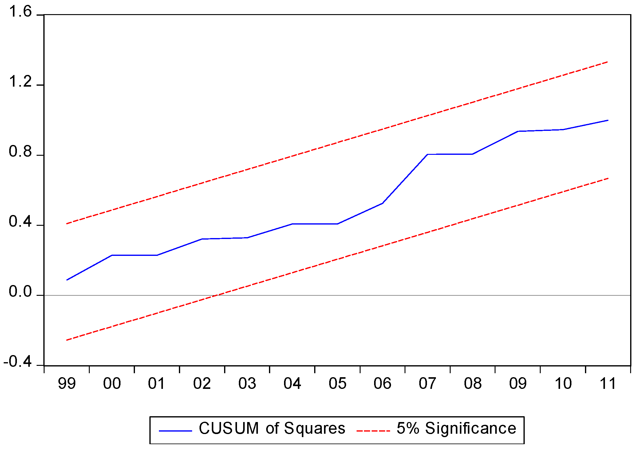
Before estimating the impact of urbanization, industrialization, services share in GDP, and income on energy intensity, we need to check for the presence of a cointegrating relationship between the variables by computing the bounds F-test statistic based on the estimation of the UECM given by Equation (7). When estimating this model, we integrate a dummy variable for each break, which takes the value one before the breakpoint date, and zero after. Therefore, the model is estimated by integrating three dummies for optimal length of the variables chosen based on the results of Akaike information criterion (AIC). We retain only the dummies that are statistically significant at 5% significance level. Results show that we have an ARDL (1, 5, 0, 4, 5). The results of bounds testing for cointegration are shown in Table 3. By estimating this model, the Wald test gives an F-statistic equal to 5.54, which is largely higher than the upper bound critical values at 10%, 5%, and 1% levels of significance given by Narayan [41]. This implies that we reject the null hypothesis of no cointegration. Hence, the variables are cointegrated when energy intensity is the dependent variable. We check the robustness of the UECM by applying some diagnostic tests. As shown in Table 3, the UECM passes all the diagnostic tests against non-normality, serial correlation, and autoregressive conditional heteroscedasticity (ARCH) of residuals and misspecification of the model. In fact, the Jarque–Bera normality test, the serial correlation LM test, and the ARCH test show that residuals are normal, not correlated, and not heteroskedastic. In addition, the Reset RAMSEY test shows that the model is not misspecified. Finally, the results of CUSUM and CUSUM of squares tests indicate that the estimates of the ARDL model are stable because Figure 4 and Figure 5 show that the cumulative sums are lying between the two critical lines (red lines).
3.3. Short- and Long-Term Elasticities
The existence of a cointegrating relationship between energy intensity, urbanization, industrialization, and income in Saudi Arabia allows the estimation of the ECM given by Equation (8) to determine the short- and long-term elasticities of the independent variables. The results of estimation of the ECM are shown in Table 4. They indicate that the coefficient of the ECT is negative and significant at a level of 1%, confirming the previous result of the bounds test for cointegration and proving the stability of this long-term relationship over the period studied. Urbanization, real GDP per capita, services share in GDP, and industrialization Granger cause energy intensity in the long term in Saudi Arabia. The coefficient of the ECT is equal to −0.99, indicating that the deviation of energy intensity from the short term to the long term is corrected by 99% each year. In addition, after a shock to energy intensity in Saudi Arabia, the convergence to equilibrium takes about one year.
Since our variables are cointegrated when energy intensity is the dependent variable, the long-term elasticity of each independent variable is determined by the estimated coefficient of one lagged level of the independent variable divided by the estimated coefficient of one lagged level of the dependent variable (energy intensity) multiplied by a negative sign [8]. Table 4 reveals positive effects of the four variables (real GDP per capita, urbanization, industrialization, and services share in GDP) on energy intensity in the long term. The three variables of urbanization, industrialization, and services are significant at the 5% level. However, only the coefficient of real GDP per capita variable is not statistically significant at the 10% level or lower in the long-term relationship equation. Hence, the combined effects of increasing income, industrialization, services, and urbanization will not lead to a fall in energy intensity in the long term in Saudi Arabia. These findings conform to those of Jones [2], Parikh and Shukla [4], Burney [3], Holtedahl and Joutz [5], York [6], Liu [27], Poumanyvong et al. [10], Shahbaz and Lean [8], Adom et al. [9], Al-mulali et al. [11] and Ma [17].
The short-term elasticities of the independent variables (real GDP per capita, urbanization, services, and industrialization) are computed here as the estimated coefficients of their first differences in the ECM given by Equation (8). As shown in Table 4, the real GDP per capita has a negative and significant impact on energy intensity in the short term. Its elasticity is equal to −1.17, indicating that a 10% increase in real GDP per capita leads to a decline of 11.7% in energy intensity in the short term. This income effect represents only the technique effect because, when the dependent variable is energy intensity, the income elasticity reflects only the technique effect and not the scale effect [16,42]. The result of the short-term income elasticity is expected; the majority of studies found this. Its value is higher than obtained by Sadorsky [16], which varied from −0.57 to −0.53.
In addition, the impact of urbanization on energy intensity is positive and significant at a level of 5% in the short term. Its elasticity of energy intensity is equal to 2.27, implying that a 1% increase in urbanization will result in an increase of 2.27% in energy intensity in the short term. At first view, this result seems reasonable for the sign of the impact. However, the higher magnitude of the impact of urbanization on energy intensity in Saudi Arabia can be explained by the rapid urbanization and the type of urbanization. It appears that urbanization has played a major role in increasing energy intensity in Saudi Arabia since the 1970s. The urbanization process has a larger elasticity on energy intensity than income. This result supports the hypothesis that urban infrastructure needs to consume more energy through the expansion of economic activities. Moreover, urbanized cities are characterized by more motorized traffic and congestion, which leads to more energy use. The vast oil reserves of Saudi Arabia have led to the economic modernization and prosperity of the country. In particular, urbanization has led production to shift from agriculture that is less energy-intensive to manufacturing industries, which are more energy-intensive. For example, the share of agriculture in GDP passed from 4.93% in 1968 to 1.80% in 2012 in Saudi Arabia [26]. Modernization of the country has also promoted modern buildings, which are operating with more energy consumption equipment (e.g., refrigerators and air conditioning). Hence, Saudi Arabia should implement some instruments that help manage urbanization and reduce energy use in cities.
We observe that industrialization and services also remain significant in the short term and have positive impacts on energy intensity. Therefore, industrialization is determinant of energy intensity for the case of Saudi Arabia. The positive elasticity of industrialization implies that increases in industrialization have led to increases in energy intensity in Saudi Arabia. This result may be explained by the fact that Saudi Arabia has passed from the agricultural-intensive economy to the petroleum industrial-intensive economy. Saudi Arabia’s industry is based on petroleum industrial activities and manufacturing. The petroleum industrial activities (e.g., petroleum refining) and manufacturing lead in general to an increase in energy consumption and hence an increase in energy intensity because they consume more energy than traditional agricultural activities or textile industries.
The positive impact of the variable services on energy intensity is not expected. It can be explained by the fact that Saudi Arabia has not attained the stage where its economy is service-intensive and services in Saudi Arabia are mainly compound of industrial services such as transport activities.
3.4. Robustness of Results
In order to check the robustness of results shown by the ARDL model, we use two other cointegration regressions: the fully modified OLS (FMOLS) of Phillips and Hansen [43] (1990) and the dynamic OLS (DOLS) of Stock and Watson [44]. They are employed with LEI as a dependent variable and LGDP, LURB, LSER, and LIND as regressors. The FMOLS method employs a semi-parametric correction to eliminate the problems caused by the long-term correlation between the cointegrating equation and stochastic regressor innovations. Its estimator is asymptotically unbiased. The DOLS is applied with lead and lag length equals to 2 and 3, respectively, which makes the stochastic error term independent of all past innovations in stochastic regressors.
Results of both methods of FMOLS and DOLS are shown in Table 5. They do not differ greatly from the earlier results shown by the ARDL model.
After estimating the long-term relationship using the methods of FMOLS and DOLS, we use the Hansen test [45] in order to check for the existence of a cointegrating relationship. This test checks the null hypothesis of cointegration against the alternative of no cointegration. The results of the test show that the probability levels are superior to 5%, indicating that we cannot reject the null hypothesis that the variables are cointegrated at conventional levels. These results confirm our previous finding of the ARDL method.
3.5. Non-Granger Causality Test of Toda and Yamamoto (1995)
In order to test the causality between energy intensity, real GDP per capita, urbanization, industrialization, and services share in GDP, we use a modified Wald test developed by Toda and Yamamoto (1995). This test avoids the problems associated with the ordinary Granger causality test when the series are integrated of different orders. The basic idea of the Toda and Yamamoto (1995) approach consists in augmenting the correct vector autoregressive (VAR) of order (p) by the maximal order of integration of the variables (dmax) and then estimates the “augmented” VAR that guarantees the asymptotic distribution of the Wald statistic [46,47].
To undertake Toda and Yamamoto [48] version of the Granger non-causality test, we estimate the augmented VAR with maximum lag order 2 to investigate the direction of causality between energy intensity, real GDP per capita, urbanization, industrialization, and services share in GDP. The results of this test are reported in Table 6. They show that there are bidirectional causality between economic activity and industrialization, bidirectional causality between real GDP per capita and services share in GDP, bidirectional causality between services share in GDP and industrialization, unidirectional causality running from urbanization to economic activity, and unidirectional causality running from energy intensity to services share in GDP. The absence of causality between urbanization and energy intensity implies that the impact of urbanization on energy intensity is occurring via economic activities. These results do not conform to those obtained by Al-mulali et al. [11], who found a bidirectional long-term causal relationship between urbanization and energy consumption in MENA countries.
4. Conclusions and Policy Implications
The impact of urbanization on energy consumption (or energy intensity) has not been studied in Saudi Arabia. All Saudi Arabia's previous studies on the topic are devoted to the analysis of the relationship between energy consumption, economic growth, and CO2 emissions. Different from previous studies, this paper analyzes the impact of urbanization, real GDP per capita, services share in GDP, and industrialization on energy intensity using an ARDL model and the Granger non-causality test over the period 1971–2012 in Saudi Arabia. Both methods have the advantage that they both avoid the bias associated with standard unit root and cointegration tests in the presence of structural change.
The bounds cointegration test suggests the existence of a long-term relationship between urbanization, industrialization, services share in GDP, economic output, and energy intensity. Moreover, the significance of the error correction term indicates that there is unidirectional Granger causality running from urbanization, economic output, services share in GDP, and industrialization to energy intensity in the long term. In addition, the estimation of the ECM indicates that urbanization positively affects energy intensity in the short term. The value of urbanization elasticity to energy intensity implies that a 1% increase in urbanization causes an increase of 2.27% in energy intensity in the short term. This result does not support the urban compaction hypothesis where urban cities benefit from economies of scale in public infrastructure. Due to the importance of the relation between urbanization and energy intensity, this result is interesting for designing energy policies because the urbanization process in Saudi Arabia leads to an increase in energy intensity. Improving energy efficiency is important in Saudi Arabia for mitigating climate change problems and releasing more quantities of energy consumed locally to be exported and hence more oil export revenues that enhance economic development. In addition, Saudi Arabia should give more attention to the economic transformation.
In light of this result, in order to slow down energy consumption and attain sustainable development in Saudi Arabia, energy policies should be based on tackling all the sources of overuse of energy. For example, measures that slow down the rapid urbanization process should be undertaken to reduce energy intensity in Saudi Arabia. A reduction in energy intensity in Saudi Arabia is urgent because it has an important role in protecting the environment through the reduction of CO2 emissions. In addition, the decrease in energy intensity can be a tool for mitigating the impacts of energy use on carbon dioxide emissions and hence on climate change through the implementation of policies based on energy savings in all sectors [16,17,18,19,20,21,22].
Supplementary Files
Supplementary File 1Acknowledgments
The research leading to this paper was sponsored by Najran University, Kingdom of Saudi Arabia (NU/ESCI/14/018).
Author Contributions
Atef Saad Alshehry collected the data whereas Mounir Belloumiconceived and performed the experiments using the analysis tools. Both authors analyzed the data and wrote the paper.
Conflicts of Interest
The authors declare no conflict of interest.
References
- Liddle, B.; Lung, S. Might electricity consumption cause urbanization instead? Evidence from heterogeneous panel long-run causality tests. Glob. Environ. Chang. 2014, 14, 42–51. [Google Scholar] [CrossRef] [Green Version]
- Jones, D.W. Urbanization and energy use in economic development. Energy J. 1989, 10, 29–44. [Google Scholar] [CrossRef]
- Burney, N. Socioeconomic development and electricity consumption. Energy Econ. 1995, 17, 185–195. [Google Scholar] [CrossRef]
- Parikh, J.; Shukla, V. Urbanization, energy use and greenhouse effects in economic development—Results from a cross-national study of developing countries. Glob. Environ. Chang. 1995, 5, 87–103. [Google Scholar] [CrossRef]
- Holtedahl, P.; Joutz, F.L. Residential electricity demand in Taiwan. Energy Econ. 2004, 26, 201–224. [Google Scholar] [CrossRef]
- York, R. Demographic trends and energy consumption in European Union Nations, 1960–2025. Soc. Sci. Res. 2007, 36, 855–872. [Google Scholar] [CrossRef]
- Mishra, V.; Smyth, R.; Sharma, S. The energy-GDP nexus: evidence from a panel of pacific island countries. Resour. Energy Econ. 2009, 31, 210–220. [Google Scholar] [CrossRef]
- Shahbaz, M.; Lean, H.H. Does financial development increase energy consumption? The role of industrialization and urbanization in Tunisia. Energy Policy 2012, 40, 473–479. [Google Scholar] [CrossRef] [Green Version]
- Adom, P.; Bekoe, W.; Akoena, S. Modelling aggregate domestic electricity demand in Ghana: An autoregressive distributed lag bounds cointegration approach. Energy Policy 2012, 42, 530–537. [Google Scholar] [CrossRef]
- Poumanyvong, P.; Kaneko, S.; Dhakal, S. Impacts of urbanization on national transport and road energy use: Evidence from low, middle and high-income countries. Energy Policy 2012, 46, 268–277. [Google Scholar] [CrossRef]
- Al-mulali, U.; Fereidouni, H.; Lee, J.; Sab, C. Exploring the relationship between urbanization, energy consumption, and CO2 emission in MENA countries. Renew. Sustain. Energy Rev. 2013, 23, 107–112. [Google Scholar] [CrossRef]
- Liddle, B. Demographic dynamics and per capita environmental impact: Using panel regressions and household decompositions to examine population and transport. Popul. Environ. 2004, 26, 23–39. [Google Scholar] [CrossRef]
- Poumanyvong, P.; Kaneko, S. Does urbanization lead to less energy use and lower CO2 emissions? A cross-country analysis. Ecol. Econ. 2010, 70, 434–444. [Google Scholar] [CrossRef]
- Fang, W.S.; Miller, S.; Yeh, C.-C. The effect of ESCOs on energy use. Energy Policy 2012, 51, 558–568. [Google Scholar] [CrossRef]
- Wang, Q. Effects of urbanization on energy consumption in China. Energy Policy 2014, 65, 332–339. [Google Scholar] [CrossRef]
- Sadorsky, P. Do urbanization and industrialization affect energy intensity in developing countries? Energy Econ. 2013, 37, 52–59. [Google Scholar] [CrossRef]
- Ma, B. Does urbanization affect energy intensities across provinces in China? Long-run elasticities estimation using dynamic panels with heterogeneous slopes. Energy Econ. 2015, 49, 390–401. [Google Scholar] [CrossRef]
- Alshehry, A.S.; Belloumi, M. Energy consumption, carbon dioxide emissions and economic growth: The case of Saudi Arabia. Renew. Sustain. Energy Rev. 2015, 41, 237–247. [Google Scholar] [CrossRef]
- Bernardini, O.; Galli, R. Dematerialization: Long term trends in the intensity of use of materials and energy. Futures 1993, 25, 431–448. [Google Scholar] [CrossRef]
- Elliot, R., Jr.; Sun, P.; Zhu, T. Urbanization and Energy Intensity: A Province-Level Study for China; Department of Economics Discussion 14-05, University of Birmingham: Birmingham, UK, 2014. [Google Scholar]
- Jones, D.W. How urbanization affects energy-use in developing countries. Energy Policy 1991, 19, 621–630. [Google Scholar] [CrossRef]
- Kanellakis, M.; Martinopoulos, G.; Zachariadis, T. European energy policy—A review. Energy Policy 2013, 62, 1020–1030. [Google Scholar] [CrossRef]
- Madlener, R.; Sunak, Y. Impacts of urbanization on urban structures and energy demand: what can we learn for urban energy planning and urbanization management? Sustain. Cities Soc. 2011, 1, 45–53. [Google Scholar] [CrossRef]
- Samouilidis, J.E.; Mitropoulos, C.S. Energy and economic growth in industrialized countries: The case of Greece. Energy Econ. 1984, 6, 191–201. [Google Scholar] [CrossRef]
- Liddle, B. The energy, economic growth, urbanization nexus across development: Evidence from heterogeneous panel estimates robust to cross-sectional dependence. Energy J. 2013, 34, 223–244. [Google Scholar] [CrossRef]
- World Development Indicators. World Bank, Washington, US. 2015. Available online: http://www.worldbank.org/data/onlinedatabases/onlinedatabases.html (assessed on 13 April 2016).
- Liu, Y. Exploring the relationship between urbanization and energy consumption in China using ARDL (autoregressive distributed lag) and FDM (factor decomposition model). Energy 2009, 34, 1846–1854. [Google Scholar] [CrossRef]
- Ewing, R.; Rong, F. The impact of urban form on U.S. residential energy use. Hous. Policy Debate 2008, 19, 1–30. [Google Scholar] [CrossRef]
- Halicioglu, F. Residential electricity demand dynamics in Turkey. Energy Econ. 2007, 29, 199–210. [Google Scholar] [CrossRef]
- Krey, V.; van O’Neill, B.C.; Ruijven, B.; Chaturvedi, V.; Daioglou, V.; Eom, J.; Jiang, L.; Nagai, Y.; Pachauri, S.; Ren, X. Urban and rural energy use and carbon dioxide emissions in Asia. Energy Econ. 2012, 34, 272–283. [Google Scholar] [CrossRef]
- O'Neill, B.C.; Ren, X.; Jiang, L.; Dalton, M. The effect of urbanization on energy use in India and China in the iPETS model. Energy Econ. 2012, 34, 339–345. [Google Scholar] [CrossRef]
- Galli, R. The relationship between energy intensity and income levels: Forecasting long-term energy demand in Asian emerging countries. Energy J. 1998, 19, 85–105. [Google Scholar] [CrossRef]
- Perron, P. The Great Crash, the Oil Price Shock, and the Unit Root Hypothesis. Econometrica 1989, 57, 1361–1401. [Google Scholar] [CrossRef]
- Hansen, B.E. The new econometrics of structural change: Dating breaks in us labor productivity. J. Econ. Perspect. 2001, 15, 117–128. [Google Scholar] [CrossRef]
- Perron, P.; Vogelsang, T.J. Nonstationarity and Level Shifts with an Application to Purchasing Power Parity. J. Bus. Econ. Stat. 1992, 10, 301–320. [Google Scholar]
- Perron, P.; Vogelsang, T.J. Testing for a Unit Root in a Time Series with a Changing Mean: Corrections and Extensions. J. Bus. Econ. Stat. 1992, 10, 467–470. [Google Scholar]
- Vogelsang, T.J.; Perron, P. Additional Test for Unit Root Allowing for a Break in the Trend Function at an Unknown Time. Int. Econ. Rev. 1998, 39, 1073–1100. [Google Scholar] [CrossRef]
- Pesaran, M.H. The role of economic theory in modeling the long run. Econ. J. 1997, 107, 178–191. [Google Scholar] [CrossRef]
- Pesaran, M.H.; Shin, Y. An autoregressive distributed lag-modeling approach to cointegration analysis. In Econometrics and Economic Theory in the 20th Century: The Ragnar-Frisch Centennial Symposium; Strom, S., Ed.; Cambridge University Press: Cambridge, UK, 1999. [Google Scholar]
- Pesaran, M.H.; Shin, Y.; Smith, R. Bounds testing approaches to the analysis of level relationships. J. Appl. Econ. 2001, 16, 289–326. [Google Scholar] [CrossRef]
- Narayan, P.K. The saving and investment nexus for China: Evidence from cointegration tests. Appl. Econ. 2005, 17, 1979–1990. [Google Scholar] [CrossRef]
- Cole, M. Does trade liberalization increase national energy use? Econ. Lett. 2006, 92, 108–112. [Google Scholar] [CrossRef]
- Phillips, P.C.B.; Hansen, B.E. Statistical Inference in Instrumental Variables Regression with I(1) Processes. Rev. Econ. Stud. 1990, 57, 99–125. [Google Scholar] [CrossRef]
- Stock, J.H.; Watson, M. A Simple Estimator Of Cointegrating Vectors In Higher Order Integrated Systems. Econometrica 1993, 61, 783–820. [Google Scholar] [CrossRef]
- Hansen, B.E. Tests for Parameter Instability in Regressions with I(1) Processes. J. Bus. Econ. Stat. 1992, 10, 321–335. [Google Scholar]
- Wolde-Rufael, Y. Electricity consumption and economic growth: a time series experience for 17 African countries. Energy Policy 2006, 34, 1106–1114. [Google Scholar] [CrossRef]
- Esso, L.J. Threshold cointegration and causality relationship between energy use and growth in seven African countries. Energy Econ. 2010, 32, 1383–1391. [Google Scholar] [CrossRef]
- Toda, H.Y.; Yamamoto, T. Statistical inference in vector autoregressions with possibly integrated process. J. Econ. 1995, 66, 225–250. [Google Scholar] [CrossRef]
Figure 1.
Trends of urban population annual growth in Saudi Arabia and the world over the period 1961–2014.
Figure 1.
Trends of urban population annual growth in Saudi Arabia and the world over the period 1961–2014.

Figure 2.
Trends of energy intensity and urbanization in Saudi Arabia over 1971–2012 (energy intensity (EI) in the left axis; urbanization (URB) in the right axis).
Figure 2.
Trends of energy intensity and urbanization in Saudi Arabia over 1971–2012 (energy intensity (EI) in the left axis; urbanization (URB) in the right axis).

Figure 3.
The plot of natural logarithms of the five variables.
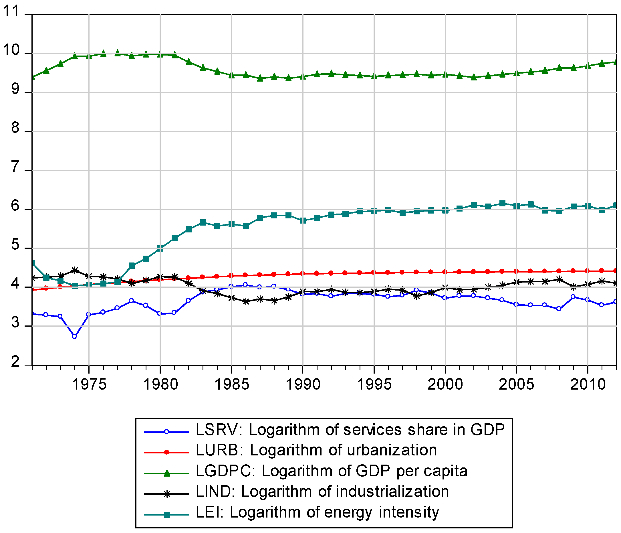
Figure 4.
Results of CUSUM test.
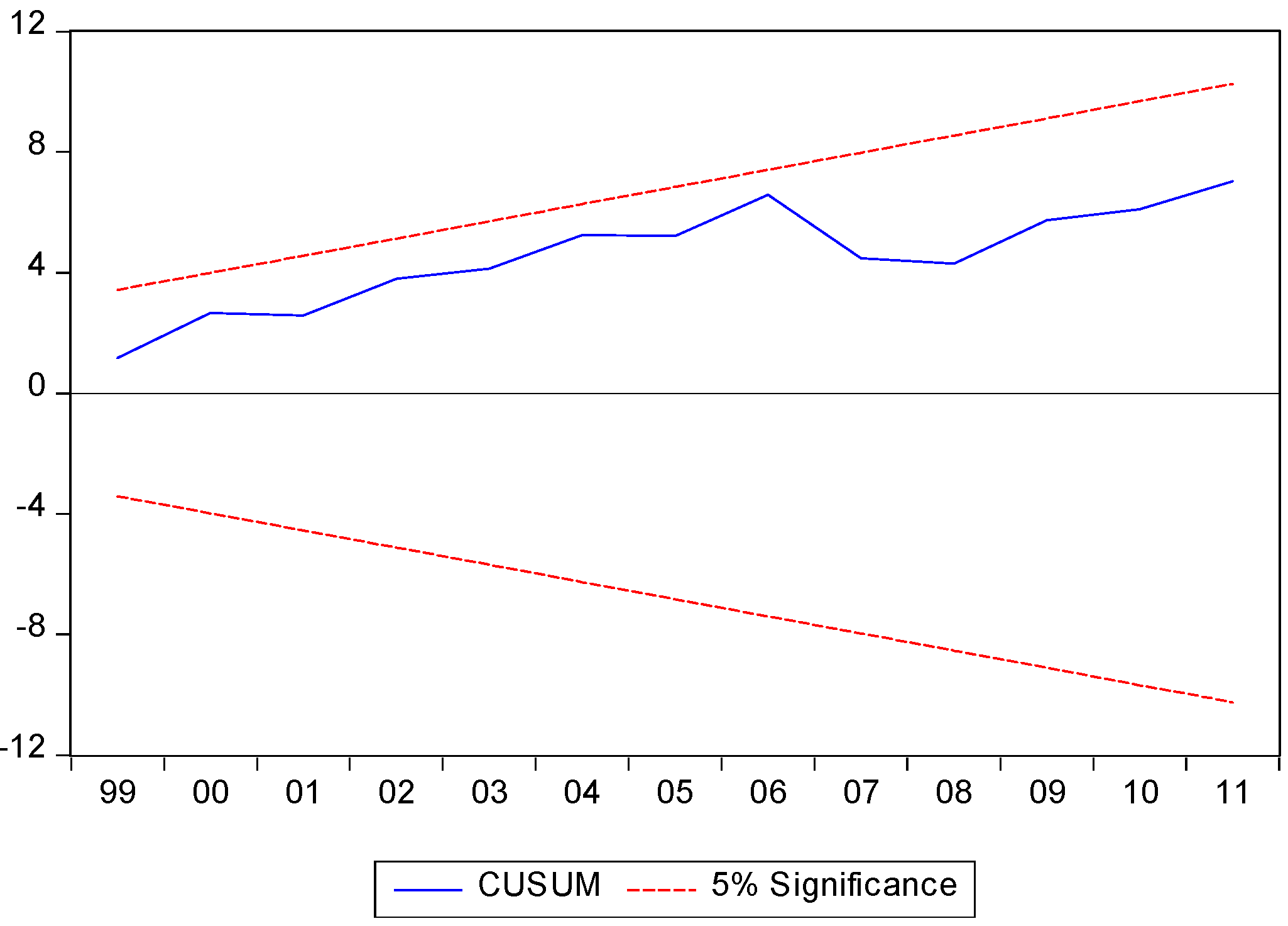
Figure 5.
Results of CUSUM of squares test.

| Variables | Levels | First differences | Order of Integration | ||||||
|---|---|---|---|---|---|---|---|---|---|
| ADF Statistic | Critical Values at 5% Level | PP Statistic | Critical Values at 5% Level | ADF Statistic | Critical Values at 5% Level | PP Statistic | Critical Values at 5% Level | ||
| LEI | 1.55 * | −1.94 | 1.02 * | −1.94 | −4.62 * | −1.94 | −4.67 * | −1.94 | I(1) |
| LGDP | −2.48 ** | −2.93 | 0.47 * | −1.94 | −3.64 * | −1.94 | −3.53 * | −1.94 | I(1) |
| LIND | −0.30 * | −1.94 | −0.29 * | −1.94 | −5.63 * | −1.94 | −5.64 * | −1.94 | I(1) |
| LSER | −2.22 ** | −2.93 | −2.14 ** | −2.93 | −7.26 * | −1.94 | −7.53 * | −1.94 | I(1) |
| LURB | −3.04 ** | −2.93 | −22.7 ** | −2.93 | I(0) | ||||
LEI: natural logarithm of energy intensity; LGDP: natural logarithm of real GDP per capita; LIND: natural logarithm of industrialization; LURB: natural logarithm of urbanization; LSER: natural logarithm of services share in GDP. * indicates that the model estimated is without constant and trend, ** model estimated is with constant. For augmented Dickey–Fuller (ADF) test, optimal lag length is chosen based on Schwarz information criterion (SIC) by considering a maximum lag equal to 9. For PP test, optimal lag length is chosen based on Newey–West bandwidth using Bartlett kernel.
| Variables | Break | Lag | ADF Test Statistic | Model | Order of Integration | |||||
|---|---|---|---|---|---|---|---|---|---|---|
| LEI | 1984 | 0 | 1.38 (0.00) | - | 0.08 (0.00) | −0.07 (0.00) | - | −7.18 [−4.52] | 3 | I(0) |
| LGDP | 1988 | 0 | 2.40 (0.00) | - | −0.01 (0.00) | 0.02 (0.00) | - | −5.19 [−4.52] | 3 | I(0) |
| LIND | 1987 | 1 | 2.47 (0.00) | - | −0.02 (0.00) | 0.03 (0.00) | - | −4.521 [−4.522] | 3 | I(1) |
| LSER | 1987 | 1 | 2.81 (0.00) | - | 0.06 (0.00) | −0.08 (0.00) | - | −5.41 [−4.52] | 3 | I(0) |
| LURB | 1984 | 9 | 1.82 (0.00) | 0.01 (0.00) | 0.008 (0.00) | −0.006 (0.00) | −0.006 (0.00) | −9.96 [−5.17] | 2 | I(0) |
Numbers in () and [] are respectively probabilities and 5% critical values.
| Dependent Variable | F-Test Statistic | Critical Values | ||||||
|---|---|---|---|---|---|---|---|---|
| 1% | 5% | 10% | ||||||
| I(0) | I(1) | I(0) | I(1) | I(0) | I(1) | |||
| 5.54 | 3.29 | 4.37 | 2.56 | 3.49 | 2.2 | 3.09 | ||
| Diagnostic tests | ||||||||
| Breusch–Godfrey Serial Correlation LM Test | χ2(1) = 2.87 (0.11) | |||||||
| Jarque–Bera Residual Normality Test | χ2(1) = 3.48 (0.17) | |||||||
| ARCH LM Test | χ2(5) = 6.87 (0.23) | |||||||
| Ramsey RESET Test | F-statistic = 0.85 (0.37) | |||||||
Critical values are given directly using Eviews 9; for diagnostic tests, the values between parentheses are probabilities.
| Regressors | Coefficient | Standard Error | t-Ratio | Probability |
|---|---|---|---|---|
| ECTt-1 | −0.99 | 0.13 | −7.58 | 0.00 |
| −1.17 | 0.24 | −4.76 | 0.00 | |
| 2.27 | 0.90 | 2.50 | 0.02 | |
| 1.10 | 0.32 | 3.42 | 0.00 | |
| 0.78 | 0.25 | 3.03 | 0.00 | |
| Co-integrating equation (long-term coefficients) | ||||
| LGDP | 0.19 | 0.24 | 0.80 | 0.43 |
| LURB | 2.50 | 0.93 | 2.68 | 0.01 |
| LIND | 4.38 | 1.27 | 3.43 | 0.00 |
| LSER | 3.84 | 1.13 | 3.38 | 0.00 |
Table 5.
Estimation results of fully modified ordinary least squares (FMOLS) and dynamic ordinary least squares (DOLS) methods.
| Regressors | FMOLS Estimates | DOSL Estimates | ||||||
|---|---|---|---|---|---|---|---|---|
| Coefficient | Std-Error | t-Ratio | Prob. | Coefficient | Std-Error | t-Ratio | Prob. | |
| LGDP | −1.01 | 0.24 | −4.08 | 0.00 | 0.09 | 0.86 | 0.11 | 0.91 |
| LURB | 4.08 | 0.33 | 12.06 | 0.00 | 5.64 | 2.62 | 2.14 | 0.06 |
| LIND | 1.47 | 0.57 | 2.54 | 0.01 | 0.93 | 5.49 | 0.17 | 0.86 |
| LSER | 0.91 | 0.40 | 2.26 | 0.02 | 0.29 | 4.96 | 0.05 | 0.95 |
| Constant | −11.49 | 3.33 | −3.44 | 0.00 | −7.67 | 7.46 | −1.02 | 0.32 |
| Dependent Variable | Wald Test Statistics (Prob. Values) | ||||
|---|---|---|---|---|---|
| LEI | LGDPC | LURB | LIND | LSER | |
| LEI | - | 0.66 (0.41) | 0.05 (0.81) | 0.49 (0.48) | 0.19 (0.65) |
| LGDPC | 0.04 (0.83) | - | 8.80 (0.00) | 11.43 (0.00) | 13.79 (0.00) |
| LURB | 1.21 (0.27) | 0.006 (0.93) | - | 1.58 (0.20) | 2.40 (0.12) |
| LIND | 1.37 (0.24) | 2.88 (0.08) | 1.44 (0.23) | - | 6.67 (0.00) |
| LSER | 3.04 (0.08) | 3.71 (0.05) | 2.54 (0.11) | 9.35 (0.00) | - |
© 2016 by the authors; licensee MDPI, Basel, Switzerland. This article is an open access article distributed under the terms and conditions of the Creative Commons Attribution (CC-BY) license (http://creativecommons.org/licenses/by/4.0/).
Share and Cite
MDPI and ACS Style
Belloumi, M.; Alshehry, A.S. The Impact of Urbanization on Energy Intensity in Saudi Arabia. Sustainability 2016, 8, 375. https://doi.org/10.3390/su8040375
AMA Style
Belloumi M, Alshehry AS. The Impact of Urbanization on Energy Intensity in Saudi Arabia. Sustainability. 2016; 8(4):375. https://doi.org/10.3390/su8040375
Chicago/Turabian StyleBelloumi, Mounir, and Atef Saad Alshehry. 2016. "The Impact of Urbanization on Energy Intensity in Saudi Arabia" Sustainability 8, no. 4: 375. https://doi.org/10.3390/su8040375
Note that from the first issue of 2016, this journal uses article numbers instead of page numbers. See further details here.