Article

Joint Environmental and Economical Analysis of Wastewater Treatment Plants Control Strategies: A Benchmark Scenario Analysis

by
Montse Meneses
*,†,
Henry Concepción
and
Ramon Vilanova
*,†
Departament de Telecomunicació i d’Enginyeria de Sistemes, Escola d’Enginyeria, Universitat Autònoma de Barcelona, 08193 Bellaterra, Barcelona, Spain
*
Authors to whom correspondence should be addressed.
These authors contributed equally to this work.
Sustainability 2016, 8(4), 360; https://doi.org/10.3390/su8040360
Submission received: 21 January 2016 / Revised: 29 March 2016 / Accepted: 6 April 2016 / Published: 13 April 2016
(This article belongs to the Section Sustainable Engineering and Science)

Abstract

:
In this paper, a joint environmental and economic analysis of different Wastewater Treatment Plant (WWTP) control strategies is carried out. The assessment is based on the application of the Life Cycle Assessment (LCA) as a method to evaluate the environmental impact and the Benchmark Simulation Model No. 1 (BSM1). The BSM1 is taken as the benchmark scenario used to implement the control strategies. The Effluent Quality Index (EQI) and the Overall Cost Index (OCI) are two indicators provided by BSM1 and used to evaluate the plant’s performance from the effluent quality and the economic points of view, respectively. This work conducts a combined analysis and assessment of ten different control strategies defined to operate a wastewater treatment plant. This analysis includes the usual economic and performance indexes provided by BSM1 joined with the LCA analysis that determines the environmental impact linked to each one of the considered control strategies. It is shown how to get an overall evaluation of the environmental effects by using a normalized graphical representation that can be easily used to compare control strategies from the environmental impact point of view. The use of only the BSM1 indexes provides an assessment that leads to a clustering of control strategies according to the cost/quality tradeoff they show. Therefore, regarding the cost/quality tradeoff, all strategies in the same group are almost equal and do not provide an indication on how to proceed in order to select the appropriate one. It is therefore shown how the fact of adding a new, complementary, evaluation (LCA based) allows either to reinforce a decision that could be taken solely on the basis of the EQI/OCI tradeoff or to select one control strategy among the others.

1. Introduction

In Europe, the implementation of the Council Directive 91/271/EEC of 21 May 1991 concerning urban wastewater treatment mandates new concepts in management and operation from the adaptation of existing plants that lack robustness and flexibility to adapt to the new requirements. In order to solve the main problems of wastewater management, researchers’ efforts have been focused, during the last few years, on objectives, such as (i) improving the water quality by also minimizing the operational costs in order to achieve sustainable treatments and (ii) minimizing the sludge production and increasing its usability for energy recovery [1,2,3].
Automatic control has been used as a support to achieve the proposed objectives. In the literature, there are several papers working on modeling of Wastewater Treatment Plants (WWTPs) [4,5,6,7]. In this work, the evaluation and comparison of the different control strategies are based on the Benchmark Simulation Model No. 1 (BSM1), developed by the International Association on Water Pollution Research and Control [8,9,10]. This benchmark defines a plant layout, influent loads, test procedures and evaluation criteria. In fact, the use of benchmarks is more and more adopted in different scenarios [11]. In this respect, WWTP operation is usually conducted on the basis of the usual cost/performance tradeoff, measured in terms of the usual Operation Costs Index (OCI) and Effluent Quality Index (EQI). In fact, this is the orientation of the usual WWTP control and operation studies, where effluent quality is one of the major concerns [12,13]. Due to implementation of the control, the general performance of Wastewater Treatment Plants (WWTPs) has been improved, but the analysis from the environmental point of view has not been detailed sufficiently. This is what raises the intention of this work by proposing to complement the existing water quality measures in terms of pollutants with the analysis of potential impacts that can be performed. This is to be accomplished by using environmental analysis techniques, such as Life Cycle Assessment (LCA) [14]. LCA is considered a convenient tool for assessing the environmental performance of WWTPs [15,16]. Some works are focused on carbon footprint; see [17], for example, as an attempt to characterize environmental impact. However, it is the authors’ opinion that LCA provides a wider and more complete perspective. In fact, LCA has been successfully used in other domains with this purpose [18,19,20]. One of the crucial points of the LCA application is an appropriate inventory definition. The inventory phase forms the core of an LCA and is the most time-consuming part. Inventory analysis involves data collection and calculation procedures to quantify relevant inputs and outputs of a production system. For instance, process inputs include raw materials, energy resources and products or semi-finished products that are the output from other processes. The quality and significance of LCA results highly depend on the quality of data that are used for the inventory analysis. Because of that, in this work, the authors have tried to perform an inventory as complete as possible, performing the quantification of all of the relevant inputs and outputs of the process.
Several LCA studies have been published on different aspects related to the water cycle: water production, water transport to the customer and wastewater treatment; however, few studies have assessed the impact of WWTP control strategies. The literature reflects studies on different aspects of the water cycle, such as potable water treatment plants [21,22], as well as several LCA studies focusing on the treatment of residual water and the technology that this requires [16]. In [23], it is illustrated how the choice of the landfill model has a significant influence on the results of life cycle assessment of waste incineration. Some studies have also carried out an environmental analysis of the urban water cycle in a city [24,25,26,27]. As an example of the combination of LCA with other techniques, such as artificial neural networks, the recent work of [28] is remarkable, showing their use for decision making in a real-time scenario. In addition it is worth mentioning the work of [29] that presents a review comparing several works, describing achievements and setting out the challenges for the coming years in the application of LCA to WWTPs. In all of these works, LCA studies on different stages of the urban water cycle have been carried out. This is why in this paper, the environmental evaluation of different control strategies, tested in BSM1, is assessed by using plant performance criteria, such as effluent quality and operational cost jointly with LCA criteria.
There are other works that apply multi-criteria analysis [11,30]; for instance, [11] improve the assessment of the N-removal performance in the BSM by implementing extended statistical entropy analysis. In recent years, the inclusion of the environmental aspect into the WWTP evaluation has increased. However, many of these studies are focused mainly on GHG emissions or Global Warming Potential (GWP). The work in [31] implements the LCA methodology within a knowledge-based Decision Support System (DSS) in order to include the environmental criteria, Eutrophication Potential (EP) and Global Warming Potential (GWP) in the decision making process when selecting the most appropriate flow diagram (PFD) for specific scenarios. It should take into account the review of [32]; this paper reviews the state of the art and the recently-developed tools used to understand and manage Greenhouse Gas (GHG) emissions form WWTPs and discusses open problems and research gaps. One of the conclusions was that the literature demonstrates that to manage WWTPs in a sustainable way, the indicators, including operational costs, net energy and multiple environmental performance measures, including GHG, have to be considered. Recent studies have demonstrated the paramount importance of applying a plant-wide approach that includes environmental aspects [1,33,34].
The combination of control simulations and LCA to evaluate the environmental plant’s performance is seen as an important contribution. The fact of assessing the application of control strategies in WWTPs from the environmental point of view using the LCA method adds a kind of natural complement to the WWTPs’ evaluation. Furthermore, it allows stakeholders to make decisions regarding the environmental consequences of the application of the control strategies on the basis of the potential impact results, because complementary information is given by this combination. This is the main motivation of the formulation of the conducted joint criteria analysis. Because of that, in this work, the environmental profile of ten control strategies implemented in the BSM1 is analyzed by using the LCA methodology.
This work shows how these different criteria, taken altogether, allow for a wider analysis and assessment of different ways to operate a wastewater treatment plant. Therefore, the objective of this work is to first define a set of potential control strategies that constitute different operational alternatives for the wastewater treatment plant. For these control strategies, a joint assessment will be conducted. It is therefore shown how this can be performed from different points of view where the fact of adding a new, complementary, evaluation allows stakeholders either to reinforce a decision that could be made solely on the basis of the EQI/OCI tradeoff or to select one control strategy among the others. In contrast with the recent study conducted in [34], a global unique environmental evaluation is provided (instead of a category by category analysis) that allows one to easily evaluate control strategies that do have better environmental behavior. This joint analysis is presented on the basis of the mentioned BSM1 scenario. This makes the conclusions for the defined control strategies site-specific. However, the fact of using a benchmark scenario provides a sense of generality, as BSM1 is intended to be a representative plant. This allows one to present the approach more from the methodological side than from the concrete numerical results; therefore, making this easily extensible to other concrete plants. The fact of using the water line scenario provided by BSM1 instead of a global plant proposal, such as in BSM2, as was done in [34], makes this generalization easier, as the control strategies are among the most widely used for the water line without further reference to other parts of the plant that otherwise may not be available (anaerobic digesters, thickeners, etc).
The article is organized as follows: First, the BSM1 and the implemented control strategies are presented in Section 2. Section 3 follows by presenting the different control strategies to be considered in the study. Section 4 presents the LCA methodology, whereas results and a comparison between control strategies are conducted in Section 5. First, the BSM1 simulation results are exposed, followed by the LCA results. In a third step, it is shown how both points of view can be joined, providing stakeholders a more complete framework to make decisions regarding the most appropriate way for plant operation. As the last section, the conclusions of the study show different alternatives for selecting the most suitable control strategies according to the exposed joint assessment.

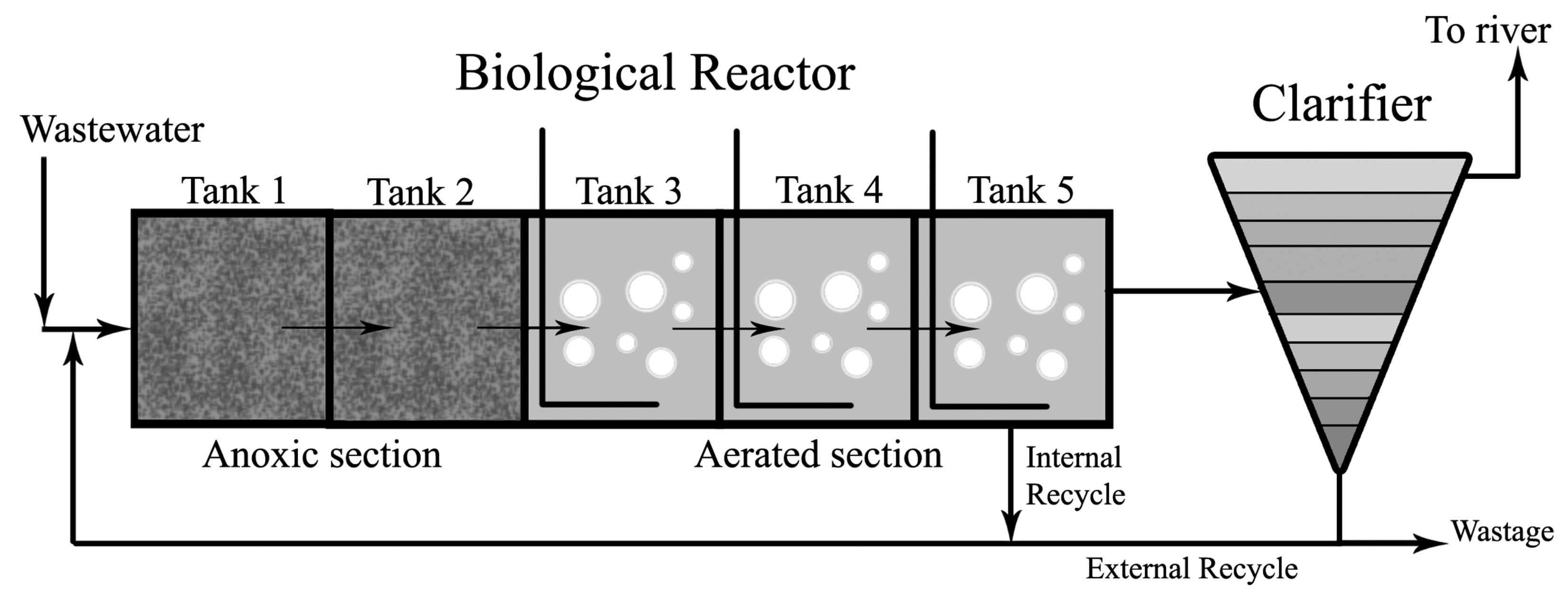
2. Benchmark Scenario: The BSM1

This section provides a description of the working scenario provided by the BSM1 [35]. This is a simulation environment defining a plant layout, a simulation model, influent loads, test procedures and evaluation criteria. BSM1 has been adopted as the simulation and benchmark framework, because most of the WWTP control strategies that can be found in the literature are based on it. These strategies are presented in the next section. Even as BSM1 has evolved to BSM2 with a more plant-wide perspective, there are not so many proposals in the literature that are defined on the BSM2 and that make use of the plant-wide concept. This is to say, these are basically water line-based strategies. From this point of view, their behavior will be reflected by acting just on the water line. This makes BSM1 a more suitable, concise and easy framework for presenting the experiments and results. Even though the authors do recognize that BSM1 is an older proposal, it is true that it is by now more established and well known among the water community.
The plant layout is composed of five activated sludge reactors in series followed by a clarifier. The first two reactors are non-aerated, but fully-mixed tanks with a total volume of 2000 m 3 . They are followed by three aerobic tanks with a total volume of 3999 m 3 , and the clarifier has a total volume of 6000 m 3 (Figure 1). The plant has been designed to treat an average influent dry-weather flow rate of 18446 m· 3 day - 1 and an average biodegradable Chemical Oxygen Demand (COD) in the influent of 300 gm - 3 . Influent data include three dynamic files used for testing dry, rain and storm conditions. The hydraulic retention time is 14.4 h, and the wastage flow rate ( Q w ) is 385 m· 3 day - 1 [35]. For modeling the nitrogen and carbon removal processes that take place in the sludge reactors, the BSM1 platform uses the Activated Sludge Model No. 1 (ASM1) [36]. As concerns the biological parameter values used in the BSM1, they correspond approximately to a temperature of 15 C . The clarifier is modeled as a non-reactive ten-layer unit with a double exponential settling velocity, as is described in [37].

2.1. Simulation Procedure

In order to ensure all BSM1 users perform the experiments under the same conditions, so that the results can be compared, a simulation protocol is established. This simulation protocol establishes how to test the plant operation strategy for the provided influent profiles (see the Appendix for a detailed description of the influent profiles). The simulation is structured into three phases. First, a 150-day period of stabilization in closed-loop using constant influent data has to be completed to drive the system to a steady state. This ensures a consistent starting point and should eliminate the influence of starting conditions on the generated dynamic output. Secondly, it continues by applying 14 days of dry influent data as a dynamic input. After this, the state variable values are saved as the starting point to evaluate the dynamic response of the plant to each dynamic influent file. Therefore, as the third step, from the achieved state, the dynamic influent file to be tested is simulated during 14 days of further simulation, but in separate studies. Only the results of the last seven days are considered for the performance assessment.

2.2. Performance Assessment

In order to compare the different control strategies, different criteria are defined. The performance assessment is made at two levels. The first level concerns the control level. Basically, this serves as a proof that the proposed control strategy has been applied properly. The second level provides measures for the effect of the control strategy at the plant level and considers quality and cost by introducing the Effluent Quality Index (EQI) and Overall Cost Index (OCI). They quantify the pollution in discharged water and the cost of operating the plant, respectively. In this work, we concentrate on these second-level indexes, as they are plant-wide defined.

2.2.1. Effluent Quality Index (EQI)

EQI (kg pollution unit ·day - 1 ) is defined [35] to evaluate the quality of the effluent. It is related to the fines to be paid due to the discharge of pollution. EQI is averaged over a seven-day observation period, and it is calculated by weighting the different compounds of the effluent loads.
E Q I = 1 1000 · T t = 7 d a y s t = 14 d a y s ( B T S S · T S S ( t ) + B C O D · C O D ( t ) + B N K j · N K j ( t ) +
+ B N O · N O ( t ) + B B O D 5 · B O D 5 ( t ) ) · Q ( t ) · d t
where T is the total time (seven days in this case) and B i are weighting factors (Table 1) for the different types of pollution to convert them into pollution units. The values for Bihave been deduced from [38].

2.2.2. Overall Cost Index

OCI (kWh·day - 1 ) is defined [35] as:
O C I = A E + P E + 5 · S P + 3 · E C + M E
where A E is the aeration energy (kWh·day - 1 ), P E is the pumping energy (kWh·day - 1 ), S P is the sludge production for disposal (kg·day - 1 ), E C is the consumption of external carbon source (kgCOD·day - 1 ) that can be added to improve denitrification and M E is the mixing energy (kWh·day - 1 ).
AE is calculated according to the following relation:
A E = S o s a t T · 1 . 8 · 1000 t = 7 d a y s t = 14 d a y s i = 1 5 V i · K L a i ( t ) · d t
where S o s a t is the oxygen saturation concentration value and V i is the volume of the tank i and K L a i the oxygen transfer rate in tank number i.
PE is calculated as:
P E = 1 T 7 d a y s 14 d a y s ( 0 . 004 · Q i n ( t ) + 0 . 008 · Q r i n ( t ) + 0 . 05 · Q w ( t ) ) · d t
SP is calculated from the TSSin the flow wastage (TSS w ) and the solids accumulated in the system:
S P = 1 T · ( T S S a ( 14 d a y s ) - T S S a ( 7 d a y s ) + T S S s ( 14 d a y s ) - T S S s ( 7 d a y s ) +
+ t = 7 d a y s t = 14 d a y s T S S w · Q w · d t )
where TSS a is the amount of solids in the reactors and TSS s is the amount of solids in the settler.
EC refers to the carbon that could be added to improve denitrification.
E C = C O D E C T · 1000 t = 7 d a y s t = 14 d a y s i = 1 i = n q E C , i · d t
where q E C , i is q E C added to compartment i, C O D E C = 400 gCOD·m - 3 is the concentration of readily-biodegradable substrate in the external carbon source.
ME is the energy employed to mix the anoxic tanks to avoid settling, and it is a function of the compartment volume:
M E = 24 T t = 7 d a y s t = 14 d a y s i = 1 5 0 . 005 · V i i f K L a i ( t ) < 20 d a y - 1 o t h e r w i s e 0 · d t

3. Implemented Control Strategies

The operation of a WWTP is based on the implementation of control loops that allow one to manipulate different variables of the system. For that purpose, feedback controllers are implemented. Whereas each feedback loop goal is to maintain a process variable, different feedback loops can be applied at the same time in order to determine the overall plant operation. After a brief presentation of the basics of a proportional integral-based control system, the basic and composite control strategies that are considered in this work are presented.

3.1. Feedback Control System

The control strategies that are presented below are based on feedback loops defined in terms of Proportional Integral (PI) controllers. PI controllers are by far the most used controllers in industry. The simplicity and good tradeoff between performance and robustness for PI controllers make them the most preferable option among practitioners. The facts of just having to adjust two parameters and its simple structure allow an easy application and tuning of the controller parameters. See [39,40] for a review on PI and PID control. The computation of the control action or manipulated variable, u ( t ) , is done according to:
u ( t ) = K p e ( t ) + 1 T i 0 t e ( τ ) d τ
where e ( t ) represents the feedback error: e ( t ) = r ( t ) - y ( t ) , y ( t ) being the controlled variable and r ( t ) its desired value or set-point. The two parameters K p and T i are, respectively, the proportional and integral gain. These parameters have to be fixed for each one of the control loops. This is usually known as the controller tuning stage [39]. Therefore, the control strategies are based on establishing the controlled and manipulated variable. As an example, Figure 2 shows a PI-based control loop where the purpose is to control the oxygen concentration in the fourth tank; in fact, as part of the control strategy predefined within the BSM1 scenario.
A typical variation of the basic feedback loop is that of a cascade control system. In this configuration, the desired value or set-point is not fixed, but determined as the output of a primary, external, controller. As an example of this configuration, in Figure 3b, we see how the dissolved oxygen set-point is determined by another PI controller that is commissioned by the desired value for the ammonia concentration at the effluent. In this case, both controllers are recognized to work on a cascade configuration.

3.2. Simple and Composite Control Strategies

The main variables to be controlled in this plant are the dissolved oxygen in the aerated tanks, the ammonia in the effluent, the nitrates in the anoxic section and the suspended solids in the effluent. These control loops can be found in the literature on WWTP control and are defined in order to achieve specific purposes on determined compound concentrations. In what follows, each one of these PI-based, basic feedback control loops is presented showing the primary reference where it was originally defined. Starting from these considerations, a set of five basic control strategies (S1 to S5) have been implemented (Figure 3).
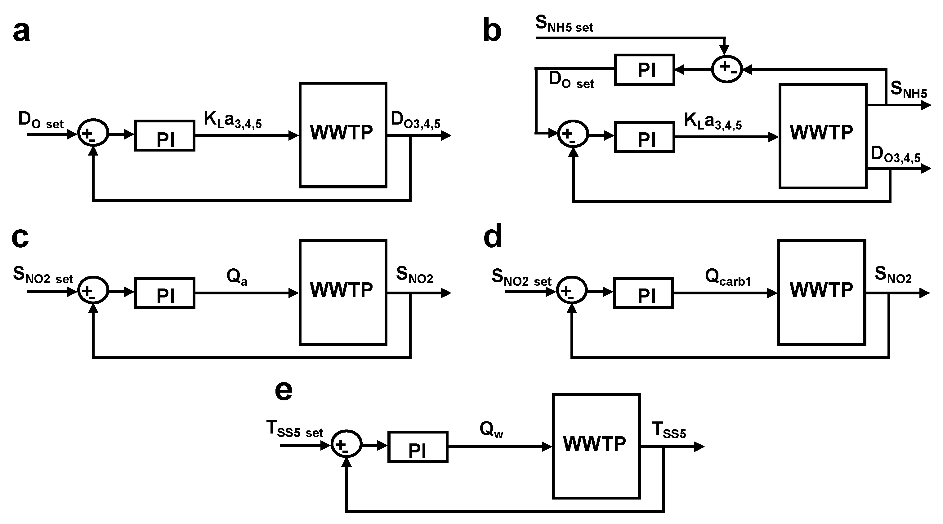
  • S1: Control of the dissolved oxygen concentration in the aerobic reactors. The controlled variables are therefore D O 3 , 4 , 5 by manipulating the respective oxygen transfer coefficients K L a 3 , 4 , 5 . In this case, three independent PI control loops are defined as shown in (Figure 3a). Details of this control strategy can be found in [35].
  • S2: Control of the ammonia in the last aerobic tank. In this case, the purpose of the controller is to maintain S N H 5 at the desired level by manipulating the oxygen set-points, D O s e t , in all of the aerobic tanks. As depicted in Figure 3b, this corresponds to a cascade control structure where the inner loops are defined along similar lines as S1. Details of this control strategy can be found in [41].
  • S3: Control of the nitrate concentration in the last anoxic tank. In this case, we are interested in controlling S N O 2 by manipulating the internal recycle flow rate Q a . This is one of the basic default control loops defined in the BSM1 scenario, as detailed in [10]. The corresponding block diagram is shown in Figure 3c.
  • S4: Control of the nitrate concentration in the last anoxic tank. In this case, we are also, as in S3, interested in controlling S N O 2 , but now, the control variable that is manipulated is the carbon source flow rate Q C a r b 1 into the first anoxic tank. The corresponding block diagram is shown in Figure 3d), whereas details on this control loop can be found in [42].
  • S5: Control of the total suspended solids concentration in the last aerobic tank; therefore, interested in keeping T S S 5 by manipulating the wastage sludge flow rate Q w . This control loop is described in [43] and shown in Figure 3e.
From the basic operation strategies S1 to S5, another five composite ones have been implemented by choosing the control of the S N H 5 strategy (S2) in order to be combined with the control of S N O 2 by manipulating Q a (S3), the control of S N O 2 by manipulating Q C a r b 1 (S4) and the control of T S S 5 (S5) strategies. Then, the control strategies S6 to S10 are defined as:
  • S6: Control of S N H 5 (S2) + control of S N O 2 by manipulating Q a (S3).
  • S7: Control of S N H 5 (S2) + control of S N O 2 by manipulating Q C a r b 1 (S4).
  • S8: Control of S N H 5 (S2) + control of T S S 5 (S5).
  • S9: Control of S N H 5 (S2) + control of S N O 2 by manipulating Q C a r b 1 (S4) + control of T S S 5 (S5).
  • S10: Control of S N H 5 (S2) + control of S N O 2 by manipulating Q a (S3) + control of T S S 5 (S5).
The details of the control strategies and the controllers used to implement them are summarized in Table 2. The implementation of all control strategies has been done by using the aforementioned Proportional Integral controllers (PI).

4. Analysis of WWTP Operation by Means of LCA

As stated, the main purpose of this study is to complement the usual BSM1 assessment indexes with an environmental impact perspective provided by the Life Cycle Assessment (LCA) technique. LCA, defined by International Standard ISO 14040 (ISO 14040, 2006) as a technique to assess the potential impacts associated with a product or process during the whole of its life cycle, involves the following steps: definition of the goal and scope, inventory analysis and impact assessment and their corresponding interpretation. In what follows, these three basic components of LCA within the scenario defined by the BSM1 are defined and specified.

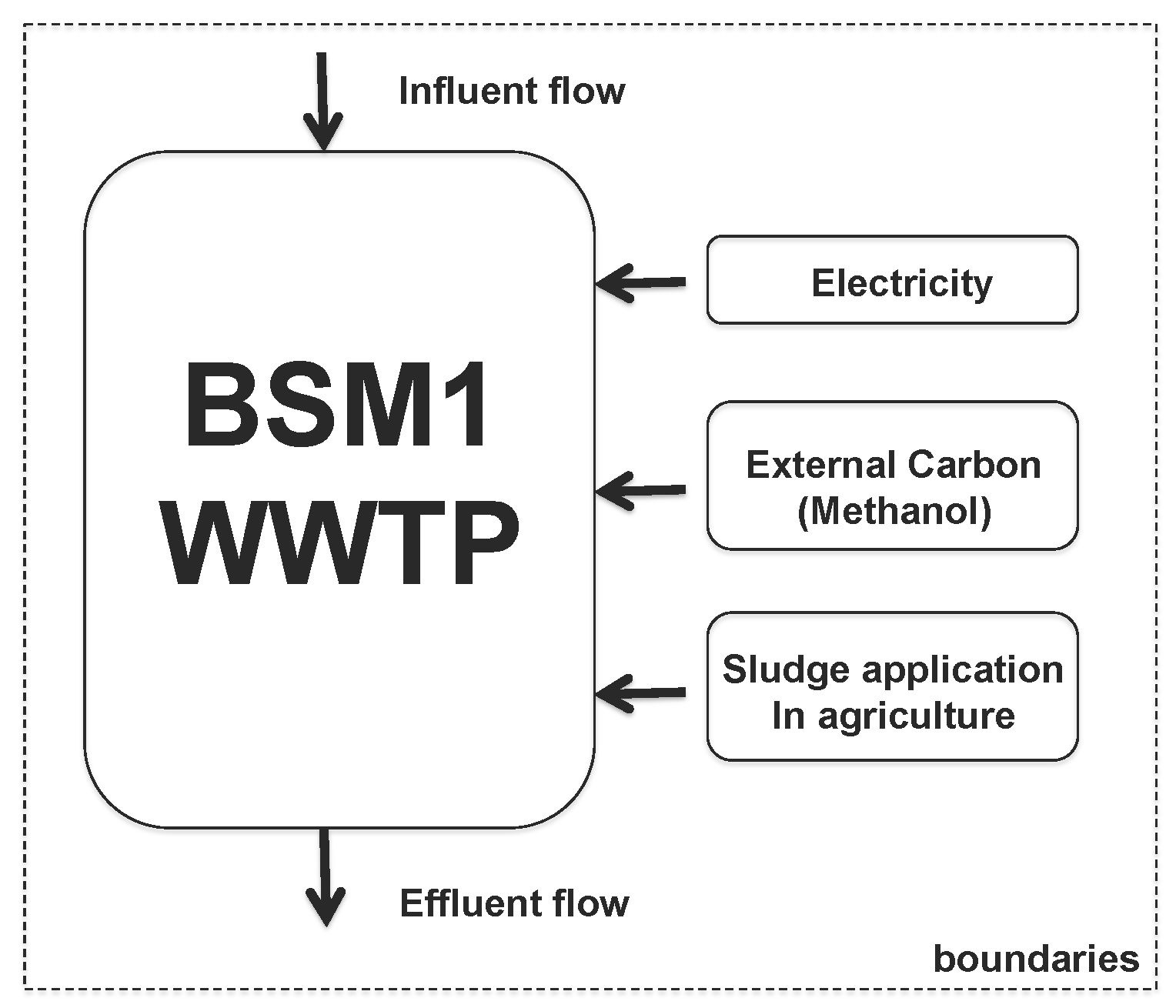
4.1. Definition of the Goal and Scope

The main objective of this LCA study is to analyze the environmental profile of the ten control strategies implemented in the BSM1 plant and to assess resulting potential impacts between the control strategies and the impact categories selected.
As the main function of WWTPs is to treat the influent to reduce organic, nutrient and suspended solid loads in order to achieve satisfactory values before the discharge of the effluent into the receiving waters, thus, referring this unit to the average influent dry-weather flow rate of the BSM1 (18,446 m 3 ·day - 1 ) and its corresponding loads, the treatment of 1 m 3 ·day - 1 of wastewater during seven days (the evaluation time of the BSM1) has been selected as the Functional Unit (FU). Therefore, the FU refers to both the amount of water and the period of time that this water is processed.
The system boundaries have been constrained just to consider the operational phase in the LCA carried out, and they have been established from “gate to gate” of the BSM1. See Figure 4. The construction phase has been excluded from the system boundaries, because the plant used is the same for all control strategies tested. However, the generation and transmission of the electricity used in the plant, the production of the chemicals used in the anoxic reactors to improve denitrification and the transportation of the generated sludge to its final destination have been included in the boundaries. The sludge considered is used in agriculture as a fertilizer, this application being one of the most common in Spain [16].

4.2. Inventory Analysis

The inventory analysis step consists of data collection and analysis of the system under study in order to quantify the inputs and outputs. The inputs and outputs are related to the use of resources (energy and raw materials) and to the release of emissions to soil, water and air. The major part of data for this study was collected from the dynamic simulations performed using the BSM1. Table 3 shows the inventory parameters used in this LCA study for each one of the implemented control strategies related to the functional unit. However, some other parts of the inventory data, that were not provided by the simulations, were collected from databases and the literature. These data are:
  • Electricity and chemicals: The electricity production data were taken from Ecoinvent Database [44] taking into account the Spanish energy production profile. In the case of the chemicals used in the BSM1 plant, methanol has been selected as the external carbon source for enhancing the denitrification process.
  • Fertilizers avoided: The application of sludge in agriculture reduces the use of chemical fertilizers. This results in benefits for the soil as long as the concentration of heavy metals in sludge is within the permitted limits [45]. The most common chemical fertilizers used in Europe are calcium ammonium nitrate (N-based) and triple superphosphate (P-based) [46]. The substitutability was assumed as 6.93 kg of triple superphosphate and 39.6 kg of calcium ammonium nitrate per ton of sludge [16].
  • Heavy metals: Heavy metals’ concentration depends mainly on the amount of industrial wastewater in the influent flow. As the BSM1 influent does not contain measures of these concentrations, an alternative source has been used: the study [45] realized in several European countries that summarizes the average of heavy metals’ concentrations that can be found in dehydrated sludge.
  • Methane and nitrogen emissions: The emissions resulting from sludge application to agriculture were calculated as in [47,48].
  • Phosphorous: ASM1 does not consider the phosphorus removal process. Nevertheless, the phosphorus in the effluent was calculated by subtracting the phosphorus concentration in the influent (166 kg·P·day - 1 ) [49] and the phosphorus concentration in the sludge, calculated as 0.04 k g · P / k g of sludge [45].
  • Sludge transportation: The transportation of sludge to the farms for agricultural purposes has been calculated by assuming that farms are located at an average of 50 km from the WWTP. Data for the calculation of the environmental loads caused by the sludge transportation in a 16-ton lorry have been taken from the Ecoinvent Database [44].

4.3. Impact Assessment

In this step of the LCA, the inputs and outputs of the inventory are analyzed, and their respective potential contributions are cataloged in terms of several impact categories. The result of the Life Cycle Impact Assessment (LCIA) is an evaluation of the product life cycle, established by the relationships between the use of resources and the release of emissions, to their respective impacts [14].
In this study, the CML2000 methodology (Version Data v2.2 (2010)), developed by the Institute of Environmental Sciences (CML) of Leiden University [50], has been used to analyze the operational impact of the implemented control strategies. This characterization model provides the characterization factors that quantify the environmental impacts of the released emissions in the corresponding impact categories. From an available wide set of impact categories, the following seven ones have been selected to perform this study, taking into account that they are commonly used in wastewater LCA studies [1,15,16]. The selected impact categories are: Acidification Potential (ADP), Global Warming Potential (GWP), Eutrophication Potential (EP), Terrestrial Ecotoxicity Potential (TAETP), Photochemical Oxidation (PHO), Depletion of Abiotic Resources (DAR) and Ozone Depletion Potential (ODP). It is worth stressing that the LCA analysis does not include any reference nor takes into account any health aspect, such as pathogens (a table has been provided as Supplementary Material that provides a short description and units of each one of the categories). It is worth mentioning that freshwater and marine toxicity impact have not been included in this study. Even though in recent years, they have been improved and have been shown to be of special interest in the case of wastewater treatment, as the BSM1 influent does not contain measures of these concentrations, they can not be included in the current scenario.

5. Results and Discussion

This section conducts the interpretation of the WWTP operation in terms of the indexes and impacts resulting from both the BSM1 scenario and the application of the LCA method. Results in terms of the EQI/OCI indexes are summarized first by grouping control strategies into groups of similar cost/quality tradeoff. Afterwards, LCA results are presented and analyzed. As there are some correlations and relations between the observed behavior of the control strategy regarding the presented analysis, in a third step, a joint analysis is conducted.

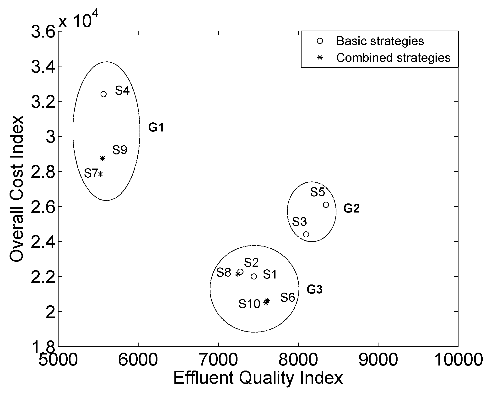
5.1. Analysis of the EQI vs. OCI Graphics

The defined control loops have been implemented and the BSM1 WWTP operated according to the established operational control strategies (S1 to S10). As a result of the performed simulations, evaluation criteria are shown in Figure 5 showing the results of the control strategies described in Section 3 in terms of EQI and OCI for the dry influent file. Taking into account these performance results, the control strategies introduced in Section 3 (as simple, S1 to S5, and composite, S6 to S10) can now be grouped according to the cost (OCI)/quality (EQI) tradeoff they show.
  • Strategies with carbon source addition (Group 1 (G1)): Strategies S4 ( S N O control in Unit 2 by manipulating Q c a r b ), S7 (combination of S2 and S4), and S9 (combination of S2, S4 and S5), are ranked with the largest OCI, but the lowest EQI (meaning a good effluent quality). Therefore, we get better water treatment, but at the expense of an associated high cost.
  • Strategies without carbon source addition and no aeration energy control (G2): Strategies S3 ( S N O control in Unit 2 by manipulating Q a ) and S5 ( T S S control in Unit 5 by manipulating Q w ), are ranked with the largest EQI value (meaning a bad effluent quality), but with a lower OCI than G1. It is straightforward to see that the small decrease in cost has a large repercussion as concerns effluent quality. This clearly reflects the impact aeration control has on the plant operation quality.
  • Strategies without carbon source addition and aeration energy control (G3): Strategies S1 ( D O control in all aerobic reactors by manipulating K L a 3 , K L a 4 and K L a 5 ), S2 ( S N H control in Unit 5 by manipulating the D O set-point in Reactors 3, 4 and 5), S6 (combination of S2 and S3), S8 (combination of S2 and S5) and S10 (combination of S2, S3 and S5). This group of strategies has the lowest OCI and a larger EQI than G1, but lower than G2, therefore showing a better tradeoff. In this case, the reduction in cost is much higher than for strategies in G2.
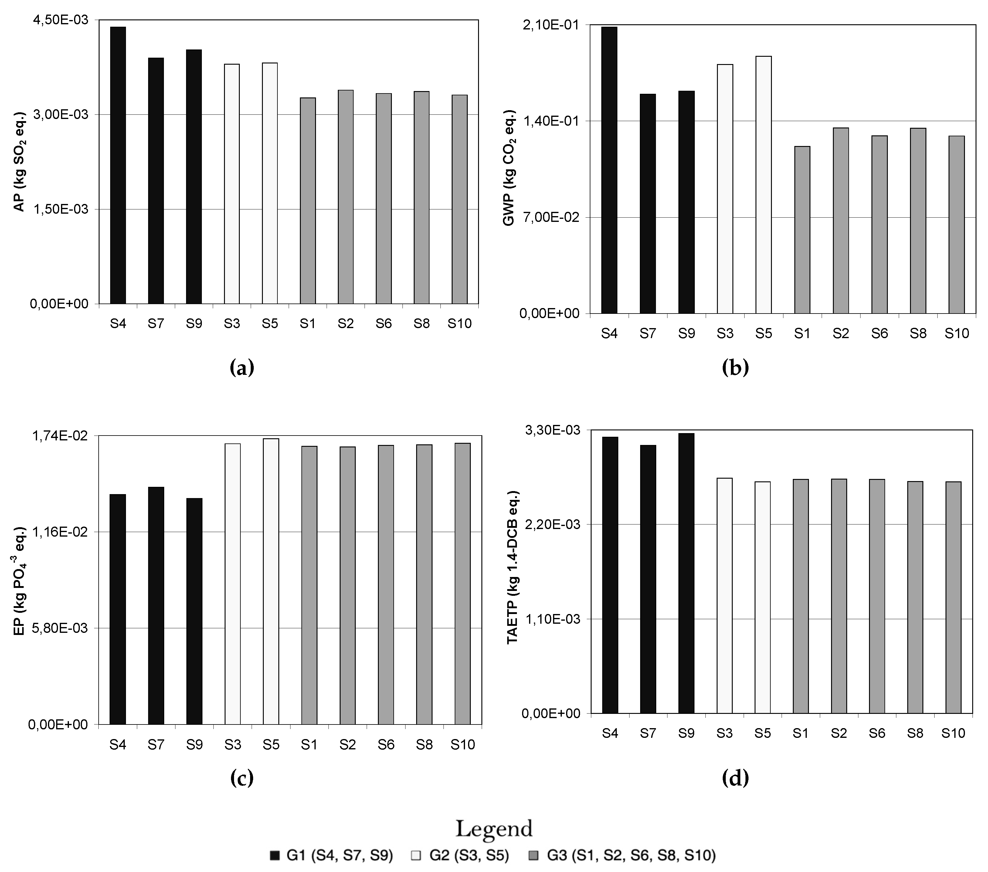
It therefore seems that the strategies of G3 provide a good cost/quality tradeoff. It is also true that there are five control strategies in this group and no clear clue for how to proceed with the appropriate choice. The next subsection provides the interpretation from the LCA perspective in order to complement the previous one and to help the decision making stage.

5.2. LCA Results

At the first stage, it should become clear that a different perspective should be adopted for the analysis of the LCA results. In fact, if we show the behavior of the different control strategies regarding a subset of the selected impact categories (AP, GWP, EP and TAEPT) and look at their behavior as members of the grouping arising from the EQI/OCI tradeoff analysis, we can see in Figure 6 that no correlation conclusion can be extracted.
S4 (Snocontrol in Unit 2 by manipulating Qcarb) presents lower eutrophication, but higher acidification potential, global warming potential and terrestrial ecotoxicity (Figure 6). As we are manipulating Qcarb, this strategy is the one with a higher consumption of carbon. In fact, all of the strategies from the group G1 with carbon source addition present a profile of lower eutrophication potential and higher terrestrial ecotoxicity potential, as well as acidification potential. Therefore, we get better water treatment, but at the expense of higher sludge production.
G3 (without carbon source addition and aeration energy control) presents a lower global warming potential and acidification potential impact (Figure 6). It should be taken into account that this strategy is the one with lower electricity consumption because of aeration energy control. Therefore, we can conclude that the aeration energy control allows us to have an important reduction in the global warming potential, acidification potential and the terrestrial ecotoxicity potential. In addition, because of the aeration control, lower values of the overall cost index are also observed.
Regarding strategies from group G2, introducing strategies without carbon source addition and no aeration energy control, they present a higher eutrophication potential impact, as well as global warming potential. The environmental benefits of using carbon addition, as have been shown in G1, are not manifested here. At the same time, as no aeration energy control is presented, these strategies do not shown the environmental benefit related to this control, as has been shown in G3. Therefore, they show the worst tradeoff.
In fact, from the environmental point of view, each one of the control strategies will have different repercussions that do not need to follow any cost or economic reason. What is desirable is to build up a figure of merit that captures the overall environmental behavior of a control strategy. In order to achieve this, first of all, each impact category has been normalized with respect to the control strategy that behaves worst (that is to say, it generates the largest environmental impact). This way, all normalized impacts will have a value between zero and one. On that basis, a control strategy that has more impacts with values closer to zero will behave better than another one with values closer to one. These normalized values have been represented using a radar chart, as this results in being very useful to display multivariate data in the form of a two-dimensional chart. Small values are closer to the origin, whereas values that are at the boundaries of the chart represent the worst behavior. The radar charts for the evaluated control strategies can be seen in Figure 7. The construction of the radar charts for environmental evaluation has been done with all impact categories having the same importance. This is in order to provide a neutral analysis. Of course, there may be cases where the geographical and/or local regulations suggest giving more importance to a particular impact category. This may be easily weighted when displaying the radar chart.
Radar diagrams shown in Figure 7 allow the environmental evaluation of control strategies, where they have been grouped as basic strategies (S1 to S5) and combined strategies (S6 to S10) for the clarity of presentation. From the first group, it is possible to identify S4 ( S N O control in Unit 2 by manipulating Q c a r b ) as the worst strategy from the environmental point of view (even though it belongs to G1 from the EQI/OCI perspective, offering the best effluent quality). In the same figure, S1 ( D O control in all aerobic reactors by manipulating K L a 3 , K L a 4 and K L a 5 ) provides a better behavior in all impact categories, except in eutrophication (the corresponding polygon is contained in all of the other strategies’ polygons).
The second figure draws two sets of strategies. S8 (combination of S2 and S5) and S10 (combination of S2, S3 and S5) have an overall better behavior in all impact categories, except for EP. As it is just in one category that they fail to be better, we can take these two as providing better overall environmental behavior. In order to choose between S8 and S10, it is seen that S10 is slightly better than S8 in two categories and at the same level in the rest.
Therefore, the environmental analysis would suggest the use of S1 (from the basic strategies) or S10 (from the composite strategies). Both control strategies belong to G3 (defined in the previous section). If now we proceed one step further with this environmental comparison and face S1 to S10, as it can be seen in Figure 8, we can find a slight advantage for S1.

5.3. Overall Joint Analysis

The two analyses previously conducted provide very different views of the control strategies’ evaluation. The EQI/OCI results suggests the grouping into the three groups according to the tradeoff they achieve. We will see in this section how taking into consideration the LCA results will allow one to go one step further and refine such categorization and to choose the best available option from the environmental point of view. It is worth noticing that this second refinement would not be possible by just looking at the numerical BSM1 standard indexes; an additional dimension is needed, and this is accomplished by the complement added with LCA.
The joint analysis to be conducted aims at joining both EQI/OCI and LCA analysis in order to get a clearer, and clever, answer regarding the choice of the appropriate control strategy. Of course, the selection will depend on the end user preferences, but the fact of having both perspectives will definitively add a wider understanding and explanation for the choice of one control strategy in front of the rest.
The joint analysis can be performed from a variety of perspectives. For example, the LCA results can take the lead and concentrate the analysis on the environmental impact. As commented in the previous subsection, the LCA results provide S1 and S10 as the best ones from the environmental point of view, showing however a quite similar overall evaluation. However, bearing in mind that S1 is the simplest control strategy, we could conclude that it is worth using S1 for providing a reasonable cost/performance tradeoff and, at the same time, the best overall environmental behavior. This view puts on the table the question regarding the suitability of implementing the additional control loops present in S10, as when we evaluate the plant operation from a plant-wide point of view, the benefits of such complex control scheme are not clear.
Another possibility is to conduct an environmental analysis within each one of the three, previously-defined, groups (G1, G2 and G3). That way, depending on the preferences on how to operate the plant (G1: high effluent quality; G2: low cost; G3: quality/cost tradeoff), adding the new dimension provided by the LCA may help to select the most appropriate one within each group. It is worth reminding that in this case, the radar diagrams are obtained by normalizing the LCA analysis with respect to the control strategies that belong to each one of the groups.
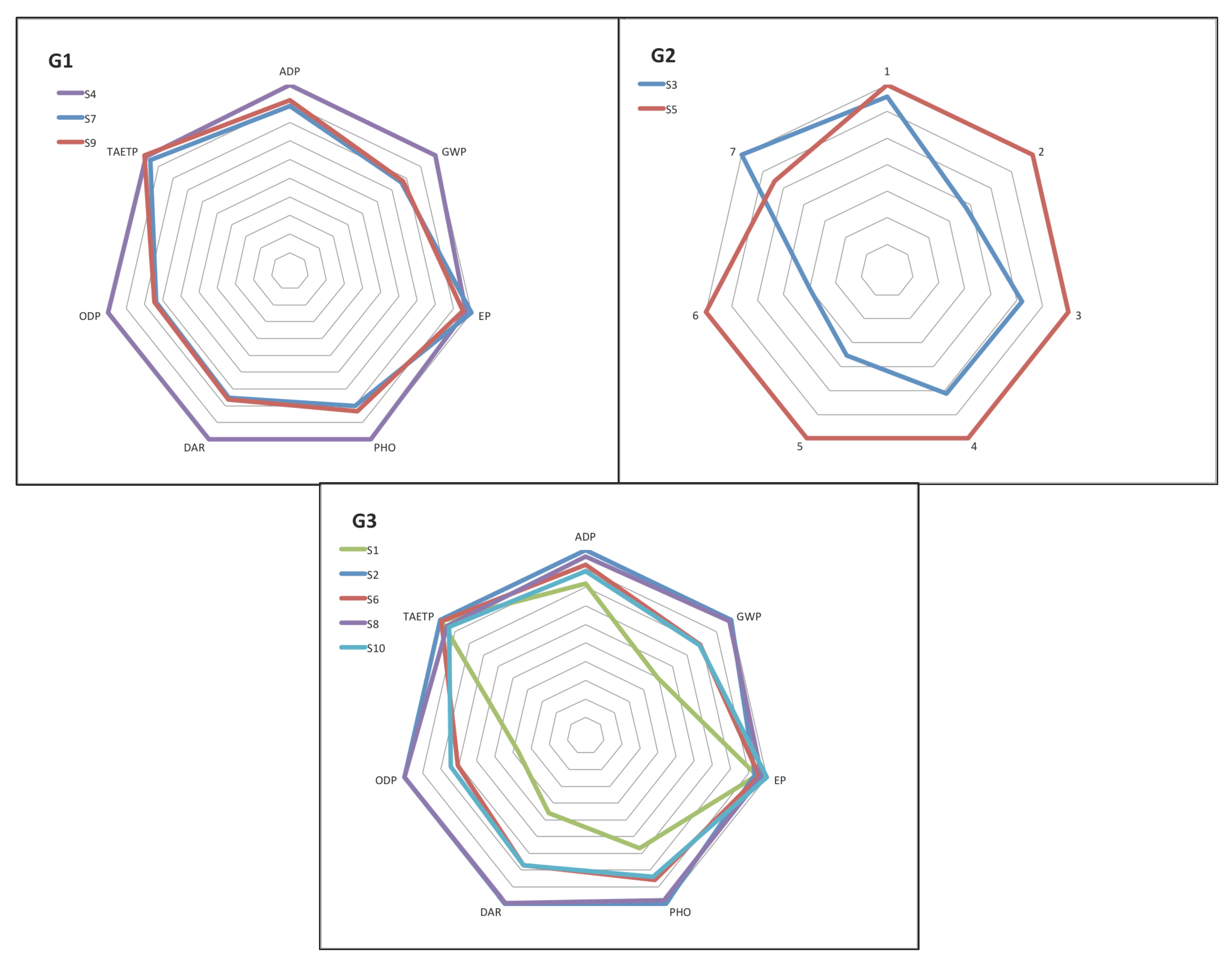
  • Group G1: High effluent quality operation. For group G1, the analysis reinforces the fact of not choosing S4 ( S N O control in Unit 2 by manipulating Q c a r b ). In fact, this strategy is the one that represents a major investment and does not provide better effluent quality than S7 (combination of S2 and S4) or S9 (combination of S2, S4 and S5). In addition, both S7 and S9 are almost identical from the environment impact they generate. The only difference is that S9 does include T S S control in addition to the control loops already present in S7. Therefore, keeping S7 would be a very good option if the plant operation is for high effluent quality.
  • Group G2: Low cost operation. For group G2, a wise selection is S3 ( S N O control in Unit 2 by manipulating Q a ). From an environmental point of view, it is drastically better, except for TAETP, than S5 ( T S S control in Unit 5 by manipulating Q w ). S3 also dominates S5 from a Pareto perspective (that is to say, it is better simultaneously in both the objectives EQI and OCI), even if slightly.
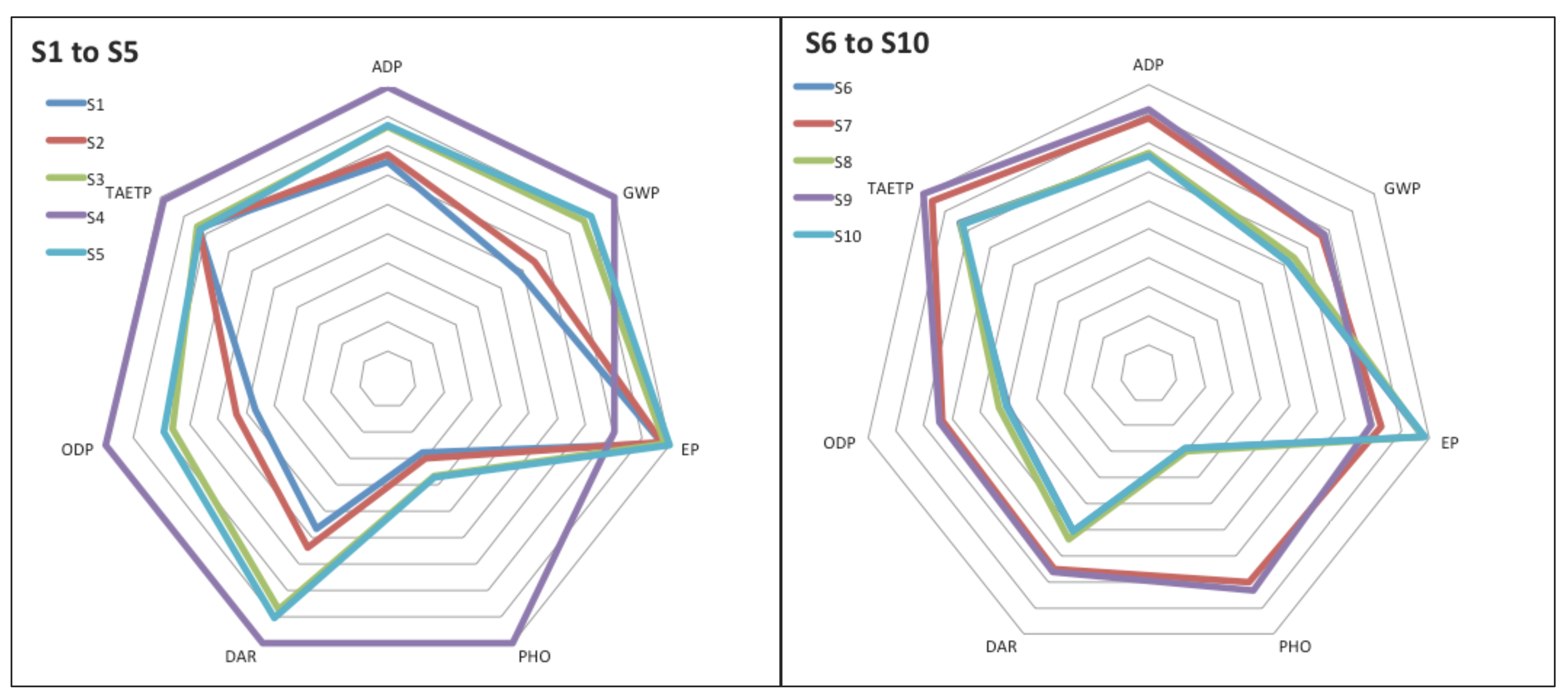
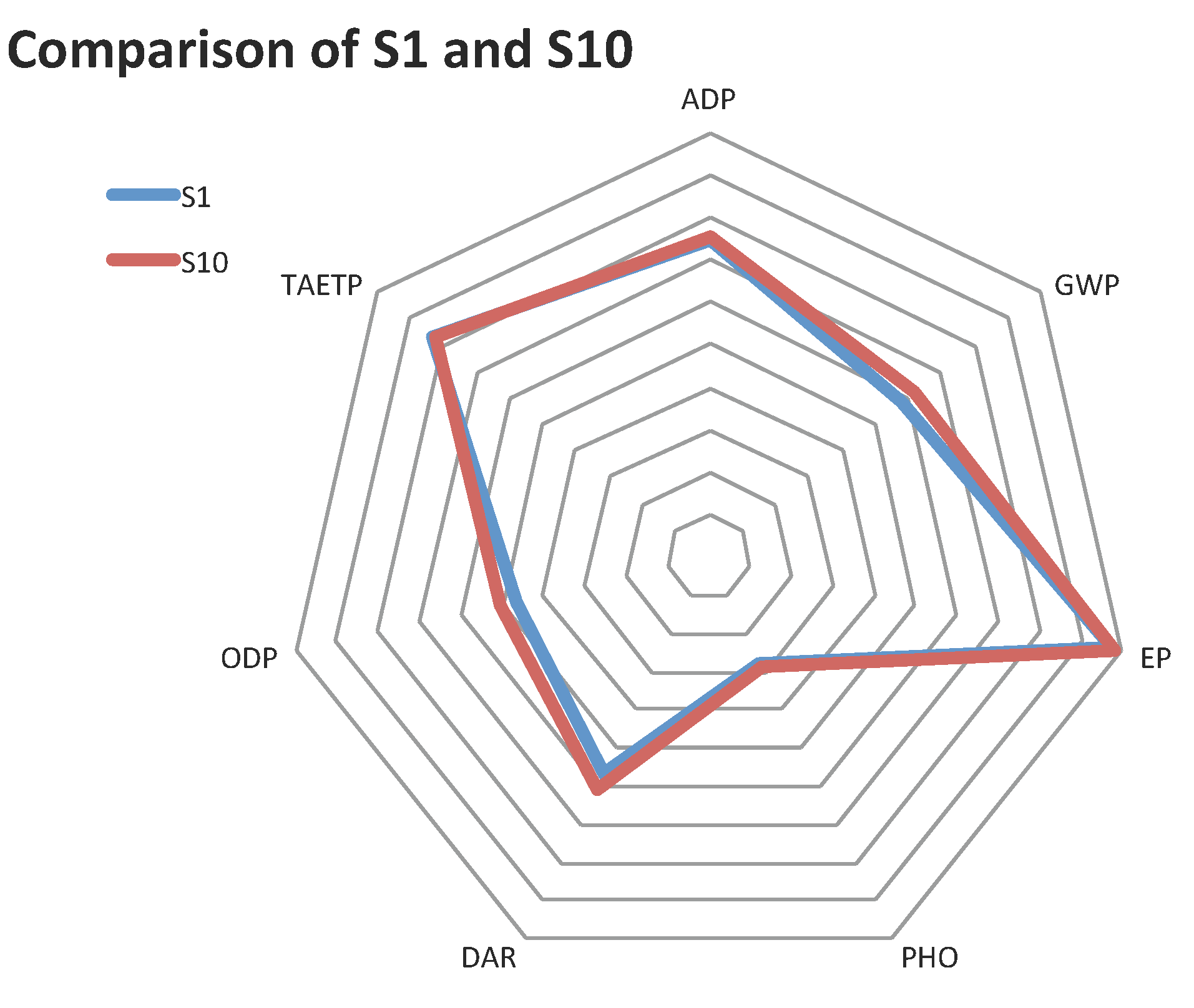
  • Group G3: Quality/cost tradeoff operation. Regarding the strategies of group G3, the decision is not clear if we just concentrate on the EQI/OCI tradeoff. There are five control strategies in this group providing similar results. Therefore, it results in being quite difficult to really choose one control strategy within the group. It is at this level of decision making where the adding of different criteria that complement the ones defined within the BSM1 benchmark helps to decide. If we can consider that from the cost/quality point of view, the five control strategies are almost equal, its behavior may not be the same if we look at the environmental side. Figure 9 provides the radar chart for the strategies of group G3. It is clear that S1 ( D O control in all aerobic reactors by manipulating K L a 3 , K L a 4 and K L a 5 ) provides a clear superior behavior regarding the environmental impact. Therefore, it justifies the application of the most simple control strategy.
For each one of these three situations, the environmental considerations allowed us to discriminate one control strategy from the corresponding group. The selected strategy provides, in addition to the kind of operation associated with the group, the most suitable operation from the environmental point of view.

6. Conclusions

This study has combined the Benchmark Simulation Model No. 1 and the life cycle assessment technique in order to evaluate the environmental and economic performance of different wastewater treatment plant control strategies. On the basis of the two complementary results, a joint assessment of wastewater treatment plant control strategies is performed.
A total of ten control strategies has been analyzed. Ranging from very simple to more complex ones, the control strategies are implemented within the BSM1 scenario, and simulation results are used to evaluate the plant performance from the cost and effluent quality points of view. In addition, LCA is applied providing a way of complementing the previous results. The overall environmental impact has been evaluated by using a normalized graphical representation that can be easily used to compare control strategies from the environmental impact point of view. The use of the standard BSM1 indexes, such as EQI/OCI, allows control strategies to be classified into three groups attending to the quality/cost tradeoff. Each one of these groups, however, does include various control strategies. The application of the environmental analysis within each group allows one to better decide on a control strategy within such a group; therefore, suggesting the one that generates less environmental impact.
From a more methodological point of view, the presented work states that the decision on the best way of operating the wastewater treatment plant, say to choose a control strategy, should not only obey aggregated indexes, such as the OCI/EQI, but include additional perspectives, such as those provided by the LCA analysis. From the aggregated indexes point of view, several control strategies provide very similar behavior; therefore, there is a need for extra decision items. Environmental impact is usually evaluated on quite different categories. The authors have shown here how to combine all of them and how to combine this extra information to help plant operators better evaluate among existing alternatives. This aspect, in the opinion of the authors, may allow stakeholders to make decisions regarding the environmental consequences of the application of the control strategies on the basis of the potential impact results, because complementary information is given by this combination.
It is worth stressing the point that all if the conducted work has been on the basis of the scenario provided by BSM1. As this comprises a particular WWTP layout, dimensions and tight characterization of plant disturbances through the provided influent data, the concrete numerical results that have been obtained are of course site specific. However, the methodological aspects of a joint analysis (environmental and operational) are considered generalizable, as BSM1 has been conceived of as representative of a typical urban wastewater treatment plant.
As future works, the authors will concentrate efforts towards analyzing the effect of the tuning changes in controllers over the simulation results and, therefore, over the environmental results obtained by the application of the LCA methodology. On the other hand, as environmental considerations are getting more and more important, a direct continuation of the work presented is that of proposing a normalize numerical index for the evaluation of the environmental impact. This numerical index would be suggested to extend and complement actual BSM1 existing assessment indexes.

Acknowledgments

This work was partially supported by the Spanish CICYT program under Grant DPI2013-47825-C3-1-R.

Author Contributions

The simulations and experiments with the WWTP scenarios were conducted by R. Concepcion, whereas M. Meneses and R. Vilanova conducted the analysis as well as designed and supervised the project. All authors contributed to the analysis and conclusions, and revised the paper. All authors read and approved the final manuscript

Conflicts of Interest

The authors declare no conflict of interest.

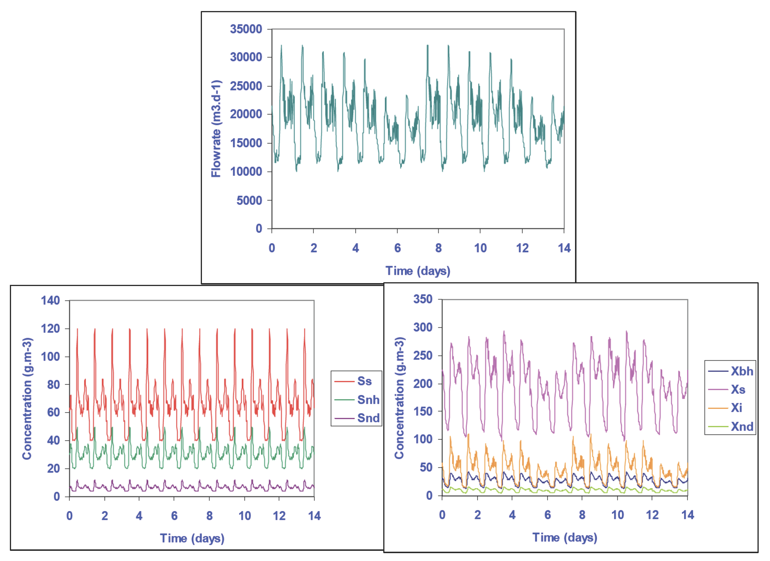
Appendix: Influent Data Profiles for BSM1

The working scenario of this paper is the one provided within the BSM1. One integral part of this scenario is the influent profiles with which the plant is fed. BSM1 provides three dynamic influent profiles corresponding to dry, rain and storm weather conditions. The influent data were initially proposed by [51] and within the BSM1 report of [10]. As explained in the main text, only the results for the dry influent are considered. Therefore, the influent profiles for this case are shown. The influent provides values for the flow rate, given in m 3 ·day - 1 , and the concentrations of the different considered components, given in g·m - 3 . Figure A1 shows the time variation if such profiles, where:
Figure A1. Influent profiles for dry weather conditions on BSM1.
Sustainability 08 00360 g010
Table A1. Influent data components.
S s Readily-biodegradable substrate
S n d Soluble biodegradable organic nitrogen
S n h N H 4 + N H 3 nitrogen
X i Particulate inert organic matter
X s Slowly-biodegradable substrate
X b , h Active heterotrophic biomass
X n d Particulate biodegradable organic nitrogen
In addition, in any influent, S o = 0 g ( - C O D ) · m - 3 (dissolved oxygen), X B , A = 0 g C O D · m - 3 (active autotrophic biomass), S N O = 0 g N · m - 3 (nitrate and nitrite nitrogen), X P = 0 g C O D · m - 3 (particulate products arising from biomass decay), S A L K = 0 m o l · m - 3 (alkalinity).

References

  1. Flores, X.; Gallego, A.; Feijoo, G.; Rodriguez-Roda, I. Multiple-objective evaluation of wastewater treatment plant control alternatives. J. Environ. Manag. 2010, 91, 1193–1201. [Google Scholar] [CrossRef] [PubMed]
  2. Gernaey, K.V.; Jeppsson, U.; Vanrolleghem, P.A.; Coop, J.; Steyer, J.P. Benchmarking of Control Strategies for Wastewater Treatment Plants; Technical Report; IWA Publishing: London: UK, 2010. [Google Scholar]
  3. Stare, A.; Vrecko, D.; Hvala, N.; Strmcnik, S. Comparison of control strategies for nitrogen removal in an activated sludge process in terms of operating costs: A simulation study. Water Res. 2003, 41, 2004–2014. [Google Scholar] [CrossRef] [PubMed]
  4. Rojas, J.D.; Baeza, J.A.; Vilanova, R. Effect of the controller tuning on the performance of the BSM1 using a data driven approach. In Proceedings of the 8th International IWA Symposium on Systems Analysis and Integrated Assessment in Water Management, San Sebastián, Spain, 20–22 June 2011.
  5. Rojas, J.; Flores, X.; Jeppson, U.; Vilanova, R. Application of multivariate virtual reference feedback tuning for wastewater treatment plant control. Control Eng. Pract. 2012, 20, 499–510. [Google Scholar] [CrossRef]
  6. Vrecko, D.; Hvala, N.; Carlsson, B. Feedforward-feedback control of an activated sludge process: A simulation study. Water Sci. Technol. 2003, 47, 19–26. [Google Scholar] [PubMed]
  7. Vrecko, D.; Hvala, N.; Stare, A.; Burica, O.; Strazar, M.; Levstek, M.; Cerar, P.; Podbevsek, S. Improvement of ammonia removal in activated sludge process with feedforward-feedback aeration controllers. Water Sci. Technol. 2006, 53, 125–132. [Google Scholar] [CrossRef] [PubMed]
  8. Alex, J.; Beteau, J.F.; Copp, J.B.; Hellinga, C.; Jeppsson, U.; Marsili-Libelli, S.; Pons, M.; Spanjers, H.; Vanhooren, H. Benchmark for Evaluating Control Strategies in Wastewater Treatment Plants. In Proceedings of European Control Conference, Karlsruhe, Germany, 31 August–3 September 1999.
  9. Alex, J.; Benedetti, L.; Copp, J.; Gernaey, K.V.; Jeppsson, U.; Nopens, I.; Pons, N.; Rieger, L.; Rosen, C.; Steyer, J.P.; et al. Benchmark Simulation Model No. 1 (BSM1); Technical Report CODEN:LUTEDX/(TEIE-7229)/1-62/(2008); Department of Industrial Electrical Engineering and Automation, Lund University: Lund, Sweden, 2008. [Google Scholar]
  10. Copp, J.B. The COST Simulation Benchmark-Description and Simulator Manual; Office for Official Publications of the European Communities: Luxembourg, Luxembourg, 2002. [Google Scholar]
  11. Sobantka, A.; Pons, M.; Zessner, M.; Rechberger, H. Implementation of Extended Statistical Entropy Analysis to the Effluent Quality Index of the Benchmarking Simulation Model No. 2. Water 2014, 6, 86–103. [Google Scholar] [CrossRef]
  12. Guerrero, J.; Guisasola, A.; Vilanova, R.; Baeza, J. Improving the performance of a WWTP control system by model-based setpoint optimisation. Environ. Model. Softw. 2011, 26, 492–497. [Google Scholar] [CrossRef]
  13. Santin, I.; Pedret, C.; Vilanova, R. Applying variable dissolved oxygen set point in a two levelhierarchical control structure to a wastewater treatment process. J. Process Control 2015, 28, 40–55. [Google Scholar] [CrossRef]
  14. ISO14040. In Environmental Management-Life Cycle Assessment-Principles and Framework; International Organization for Standardization: Geneva, Switzerland, 2006.
  15. Gallego, A.; Hospido, A.; Moreira, M.T.; Feijoo, G. Environmental Performance of Wastewater Treatment Plants for Small Populations. Resour. Conserv. Recycl. 2008, 52, 931–940. [Google Scholar] [CrossRef]
  16. Pasqualino, J.C.; Meneses, M.; Abella, M.; Castells, F. LCA as a Decision Support Tool for the Environmental Improvement of the Operation of a Municipal Wastewater Treatment Plant. Environ. Sci. Technol. 2009, 43, 3300–3307. [Google Scholar] [CrossRef] [PubMed]
  17. Chai, C.; Zhang, D.; Yu, Y.; Feng, Y.; Sing Wong, M. Carbon Footprint Analyses of Mainstream Wastewater Treatment Technologies under Different Sludge Treatment Scenarios in China. Water 2015, 7, 918–938. [Google Scholar] [CrossRef]
  18. Pushkar, S. Life Cycle Assessment of Flat Roof Technologies for Office Buildings in Israel. Sustainability 2016. [Google Scholar] [CrossRef]
  19. Shen, X.; Kommalapati, R.R.; Huque, Z. The Comparative Life Cycle Assessment of Power Generation from Lignocellulosic Biomass. Sustainability 2015, 7, 12974–12987. [Google Scholar] [CrossRef]
  20. Arzoumanidis, I.; Raggi, A.; Petti, L. Considerations When Applying Simplified LCA Approaches in the Wine Sector. Sustainability 2014, 6, 5018–5028. [Google Scholar] [CrossRef]
  21. Barrios, R.; Siebel, M.; van der Helm, A.; Bosklopper, K.; Gijzen, H. Environmental and financial life cycle impact assessment of drinking water production at Waternet. J. Clean. Product. 2008, 16, 471–476. [Google Scholar] [CrossRef]
  22. Hospido, A.; Moreira, M.; Fernandez-Couto, M.; Feijoo, G. Environmental performance of a municipal wastewater treatment plant. Int. J. LCA 2004, 9, 261–271. [Google Scholar] [CrossRef]
  23. Hellweg, S.; Hofstetter, T.; Hungerbühler, K. Modeling Waste Incineration for Life-Cycle Inventory Analysis in Switzerland. Environ. Model. Assess. 2001, 6, 219–235. [Google Scholar] [CrossRef]
  24. Lim, S.; Park, J. Environmental impact minimization of a total wastewater treatment network system from a life cycle perspective. J. Environ. Manag. 2008, 90, 1454–1462. [Google Scholar] [CrossRef] [PubMed]
  25. Meneses, M.; Pasqualino, J.C.; Céspedes-Sánchez, R.; Castells, F. Alternatives for Reducing the Environmental Impact of the Main Residue From a Desalination Plant. J. Ind. Ecol. 2010, 14, 512–527. [Google Scholar] [CrossRef]
  26. Muñoz, I.; Rodríguez, A.; Rosal, R.; Fernandez-Alba, A. Life cycle assessment of urban wastewater reuse with ozonation as tertiary treatment: A focus on toxicity related impacts. Sci. Total Environ. 2009, 407, 1245–1256. [Google Scholar] [CrossRef] [PubMed]
  27. Pasqualino, J.C.; Meneses, M.; Castells, F. Life Cycle Assessment of Urban Wastewater Reclamation and Reuse Alternatives. J. Ind. Ecol. 2011, 15, 49–63. [Google Scholar] [CrossRef]
  28. Vimal, K.; Vinodh, S. LCA Integrated ANP Framework for Selection of Sustainable Manufacturing Processes. Environ. Model. Assess. 2015. [Google Scholar] [CrossRef]
  29. Corominas, L.; Foley, J.; Guest, S.; Hospido, A.; Larsen, H.F.; Morera, S.; Shaw, A. Life Cycle assessment applied to wastewater treatment: State of the art. Water Res. 2013, 47, 5480–5492. [Google Scholar] [CrossRef] [PubMed]
  30. Bordons, C.; García-Torres, F.; Valverde, L. Optimal energy management for renewable energy microgrids. RIAI-Revista Iberoamericana de Automática e Informática Industrial 2015, 12, 117–132. [Google Scholar] [CrossRef]
  31. Garrido-Baserba, M.; Hospido, A.; Reif, R.; Molinos-Senante, M.; Comas, J.; Poch, M. Including the environmental criteria when selecting a wastewater treatment plant. Environ. Model. Softw. 2014, 56, 74–82. [Google Scholar] [CrossRef]
  32. Mannina, G.; Ekama, G.; Caniani, D.; Cosenza, A.; Esposito, G.; Gori, R.; Garrido-Baserba, M.; Rosso, D.; Olsson, G. Greenhouse gases from wastewater treatment? A review of modeling tools. Sci. Total Environ. 2016, 56, 551–552. [Google Scholar]
  33. Corominas, L.; Larsen, H.; Flores-Alsina, X.; Vanrolleghem, P. Including Life Cycle Assessment for decision-making in controlling wastewater nutrient removal systems. J. Environ. Manag. 2013, 128, 759–767. [Google Scholar] [CrossRef] [PubMed]
  34. Meneses, M.; Concepción, H.; Vrecko, D.; Vilanova, R. Life Cycle Assessment as an environmental evaluation tool for control strategies in wastewater treatment plants. J. Clean. Product. 2015, 107, 653–661. [Google Scholar] [CrossRef]
  35. Alex, J.; Benedetti, L.; Copp, J.B.; Gernaey, K.V.; Jeppsson, U.; Nopens, I.; Pons, M.N.; Rieger, L.; Rosen, C.; Steyer, J.P.; et al. Benchmark Simulation Model No. 1 (BSM1). 2008. Available online: http//www.iea.lth.se/publications/Reports/LTH-IEA-7229.pdf (accessed on 8 April 2016.).
  36. Henze, M.; Gujer, W.; Mino, T.; van Loosdrecht, M.C.M. Activated Sludge Models ASM1, ASM2, ASM2d and ASM3; Technical Report; IWA Publishing: London, UK, 2000. [Google Scholar]
  37. Takács, I.; Patry, G.G.; Nolasco, D. A dynamic model of the clarification thickening process. Water Res. 1991, 25, 1263–1271. [Google Scholar] [CrossRef]
  38. Vanrolleghem, P.; Jeppsson, U.; Carstensen, J.; Carlsson, B.; Olsson, G. Integration of WWT plant design and operation - A systematic approach using cost functions. Wat. Sci. Tech. 1996, 34, 159–171. [Google Scholar] [CrossRef]
  39. Vilanova, R.; Visioli, A.E. PID Control in the Third Millennium: Lessons Learned and New Approaches; Advances in Industrial Control, ISBN 978-1-4471-2424-5; Springer: Berlin, Germany, 2012. [Google Scholar]
  40. Alcántara, S.; Pedret, C.; Vilanova, R. On the model matching approach to PID design: Analytical perspective for robust servo/regulator tradeoff tuning. J. Process Control 2010, 5, 596–608. [Google Scholar] [CrossRef]
  41. Lindberg, C.F.; Carlsson, B. Nonlinear and set-point control of the dissolved oxygen concentration in an activated sludge process. Water Sci. Technol. 1996, 34, 135–142. [Google Scholar] [CrossRef]
  42. Yuan, Z.; Bogaert, H.; Vanrolleghem, P.; Thoeye, C.; Vansteenkiste, G.; Verstraete, W. Control of external carbon addition to predenitrifying systems. J. Environ. Eng. 1997, 123, 1080–1086. [Google Scholar] [CrossRef]
  43. Lech, R.F.; Grady, C.P.L.; Lim, H.C.; Koppel, L.B. Automatic control of the activated sludge process-II. Efficacy of control strategies. Water Res. 1978, 12, 91–99. [Google Scholar] [CrossRef]
  44. Swiss Center for Life-Cycle Inventories. Ecoinvent Database. 2009. Available online: http//www.ecoinvent.org (accessed on 8 April 2016).
  45. European Commission. European Commission, Environmental, Economic and Social Impacts of the Use of Sewage Sludge on land Final Report Part II: Report on Options and Impacts. 2008. Available online: http://ec.europa.eu/environment/archives/waste/sludge/pdf/part_ii_report.pdf (accessed on 8 April 2016).
  46. Eurostat. Agricultural Statistics. Main Results-2006–2007. Available online: http://ec.europa.eu/eurostat/documents/3930297/5962526/KS-ED-08-001-EN.PDF/185d1969-b77a-4791-b29d-5af9ee774e3b (accessed on 8 April 2016).
  47. Lundin, M.; Bengtsson, M.; Molander, S. Life Cycle Assessment of Wastewater Systems: Influence of system Boundaries and Scale on Calculated Environmental Loads. Int. J. Life Cycle Assess. 2000, 34, 57–64. [Google Scholar] [CrossRef]
  48. Hobson, J. CH4 and N2O Emissions from Waste Water Handling. Good Practice Guidance and Uncertainty Management in National Greenhouse Gas Inventories. Available online: http://www.ipcc-nggip.iges.or.jp/public/gp/bgp/5_2_CH4_N2O_Waste_Water.pdf (accessed on 8 April 2016).
  49. Gernaey, K.V.; Jorgensen, S.B. Benchmarking combined biological phosphorus and nitrogen removal wastewater treatment process. Control Eng. Pract. 2004, 12, 357–373. [Google Scholar] [CrossRef]
  50. Guinée, J.; Gorrée, M.; Heijungs, R.; Huppes, G.; Kleijn, R.; de Koning, A.; van Oers, L.; Wegener Sleeswijk, A.; Suh, S.; Udo de Haes, H.; et al. Handbook on Life Cycle Assessment. Operational Guide to the ISO Standards. I: LCA in Perspective. IIa: Guide. IIb: Operational annex. III: Scientific Background; Kluwer Academic Publishers: Dordrecht, The Netherlands, 2001. [Google Scholar]
  51. Vanhooren, H.; Nguyen, K. Development of a Simulation Protocol for Evaluation of Respirometry-Based Control Strategies; University of Gent: Gent, Belgium; University of Ottawa: Ottawa, QC, Canada, 1996. [Google Scholar]
Figure 1. Benchmark Simulation Model No. 1 (BSM1) plant layout.
Sustainability 08 00360 g001
Figure 2. Example of a PI control loop for keeping the oxygen concentration of the fourth tank at a predetermined level ( S O 4 s e t ) by manipulating the oxygen transfer coefficients of the three aerated tanks ( K L a 3 , K L a 4 , K L a 5 ).
Sustainability 08 00360 g002
Figure 3. Basic control strategies: (a) Strategy 1 (S1): oxygen PI controller; (b) S2: ammonia PI controller; (c) S3: nitrate PI controller (handling Q a ); (d) S4: nitrate PI controller (handling Q c a r b 1 ); (e) S5: total suspended solids PI controller.
Sustainability 08 00360 g003
Figure 4. LCA system under study showing boundaries.
Sustainability 08 00360 g004
Figure 5. Effluent Quality Index (EQI) ( k g p o l l u t i o n u n i t s · d a y - 1 ) vs. the Overall Cost Index (OCI) ( k W h · d a y - 1 ) results for the dry influent file.
Sustainability 08 00360 g005
Figure 6. Total impact of strategies (by group) in the selected categories. (a) Acidification; (b) Global warming; (c) Eutrophication and (d) Terrestrial ecotoxicity.
Sustainability 08 00360 g006
Figure 7. Environmental evaluation of control strategies. Basic strategies (S1 to S5) and combined strategies (S6 to S10). The radar diagrams are based on normalized impact values. The best results correspond to points closer to the origin.
Sustainability 08 00360 g007
Figure 8. Environmental comparison of control strategies S1 ( D O control in all aerobic reactors by manipulating K L a 3 , K L a 4 and K L a 5 ) and S10 (combination of S2, S3 and S5).
Sustainability 08 00360 g008
Figure 9. LCA results interpretation within each one of the three EQI/OCI control strategies groups, G1, G2 and G3.
Sustainability 08 00360 g009
Table 1. B i values.
Factor B TSS B COD B NKj B NO B BOD 5
Value (g pollution unit·g - 1 )2130102
Table 2. Description of the control strategies implemented.
Characteristics 3 D O S NH Q a Q carb T SS
ControllerCascade ControllerControllerControllerController
[35][41][10][42][43]
Controlled variable D O 3 , 4 , 5 2, 2 and 2 S N H 5 S N O 2 S N O 2 T S S 5
Set-point (gm - 3 )(variable in S N H cascade controller)1114000
Manipulated variable K L a 3 , 4 , 5 3 D O set-point Q a Q c a r b 1 Q w
Control algorithmPICascade PIPIPIPI
Used in control strategyS1, S2, S6, S7 S8, S9 and S10S2, S6, S7 S8, S9 and S10S3, S6 and S10S4, S7 and S9S5, S8, S9 and S10
Table 3. Inventory data for the evaluated control strategies. All data have been normalized with respect to the chosen functional unit (the treatment of 1 m 3 ·day - 1 of wastewater during 7 days). COD, Chemical Oxygen Demand.
StrategiesS1S2S3S4S5S6S7S8S9S10
Inputs
From the background system
Electricity (kWh)0.210.220.310.310.310.220.240.220.240.22
Carbon source (kg)0000.08000.0600.060
Outputs
Emissions to soil
Sludge for disposal (kg)0.120.120.120.150.120.120.140.120.150.12
Heavy metals in the sludge
Cd (mg)1.231.231.231.451.211.231.411.221.471.22
Cr (mg)124124124145122124141123148122
Cu (mg)124124124145122124141123148122
Hg (mg)1.231.231.231.451.211.231.411.221.471.22
Ni (mg)37373743363742364436
Pb (mg)92929210991921069111191
Zn (mg)309309309363304309353306369306
Emissions to water
Total COD (g)49494950494950494949
Total BOD(g)2.82.82.83.12.82.83.12.83.02.8
NO 3 (g)12.712.314.87.3715.413.27.1212.26.9513.2
S N H (g)1.271.280.981.220.911.211.451.211.851.14
Total N (organic) (g)2.012.011.992.142.032.012.122.022.082.02
Phosphorus (g)4.064.064.073.204.154.073.354.113.104.12
Heavy metals in the effluent
Cd (mg)0.140.140.140.150.140.140.150.140.140.14
Cr (mg)13.913.913.915.114.313.914.714.114.114.1
Cu (mg)13.913.913.915.114.313.914.714.114.114.1
Hg (mg)0.140.140.140.150.140.140.150.140.140.14
Ni (mg)4.184.184.184.524.284.184.414.234.214.23
Pb (mg)10.510.510.511.310.710.511.010.610.510.6
Zn (mg)34.934.934.837.735.734.936.835.335.135.3
Emissions to air
CH 4 (g)0.620.620.620.720.600.620.710.610.740.61
N 2 O (g)0.060.060.060.070.060.060.070.060.070.06
NH 3 (g)1.211.211.211.421.191.211.391.201.451.20

