Revealed Preference and Effectiveness of Public Investment in Ecological River Restoration Projects: An Application of the Count Data Model

Abstract

Ecological river restoration projects aim to revitalize healthy and self-sustaining river systems that can provide irreplaceable benefits to human society. Cheonggyecheon and Anyangcheon are two sites of recent river restoration projects in Korea. To assess the economic value of two rivers, count data was collected to conduct the individual travel cost method (ITCM) in this study. Five statistical models such as the Poisson, the negative binomial, the zero-truncated Poisson, the negative binomial, and negative binomial model adjusted for both truncation and endogenous stratification were used in the analysis due to the nature of count data. Empirical results showed that regressors were statistically significant and corresponded to conventional consumer theory. Since collected count data indicated over-dispersion and endogenous stratification, the adjusted Negative Binomial was selected as an optimal model to analyze the recreational value of Cheonggyecheon and Anyangcheon. Estimates of the annual economic value of two river restoration projects were approximately US $170.1 million and US $50.5 million, respectively.

1. Introduction

Healthy and self-sustaining river and stream systems provide various irreplaceable benefits, which we often treat as ecosystem goods and services including abiotic (e.g., water) and biotic components (e.g., fishes), that enable the sustainability of human life [1,2]. Unfortunately, anthropogenic pressures (e.g., economic growth) have aggravated these services and growing concerns over sustaining river and stream systems have become a global problematic issue. Ironically, those activities and concerns have stimulated environmental engineering technologies on major restoration efforts. Indeed, river and stream restoration projects to sustain their services have become a worldwide phenomenon and a blooming construction business [3,4,5]. For instance, more than 10 billion dollars have been spent by public and private groups for more than 30,000 U.S. river restoration projects alone [6]. Legal mandates (e.g., the Clean Water Act in the United States and the Water Framework Directive in the European Union) also accelerate river restoration projects [7].

Many river restoration projects are primarily aimed at improving environmental conditions by investing massive amounts of public spending but, in fact, many ironically worsen natural environmental conditions near the watershed. For example, protecting infrastructure and creating river-side parks in the name of riverfront revitalization may be successful in blooming local economy but may degrade and constrain natural river and floodplain processes [8]. Unfortunately, most on-going or completed river restoration projects around the world have concentrated to meet both environmental and economic goals which are controversial targets to achieve simultaneously. In addition, such projects are being conducted conventionally by either central or local government aimed at specific targets and purposes with billions in public investments. In these regards, suspicions can be raised on how to categorize successful achievement among those numerous projects around the world. Is it worth investing in such massive public spending? Is there an efficient way to spend public assets for restoring degraded rivers with artificial construction?

Since restoring the rivers has been recognized as an imperative circumstance, Palmer et al. [5] suggested five criteria for measuring success for those who are implementing projects. Their research concluded that the most effective ecological river restoration project should lie at the intersection of ecological, stakeholder, and learning success. However, they have underestimated the value of economic success of projects. In this research, we have a keen interest on those economic values of river restoration projects because no restoration projects are free from economic assessment since investments have come from the public.

There is a wide range of studies that have investigated the economic value of restoration projects using various valuation methods, including the contingent valuation method with survey data and the travel cost method with count data. The latter, called the revealed preference method, is widely used to analyze the consumer welfare attributable to quality improvement on a recreation site. It is adequate to apply this method to analyze the consumer welfare in monetary values for ecological river restoration projects because the major economic gain from the project comes from the quality improvement of recreation. In this sense, we can trace out the demand curve for recreation at the river. One of the well-known studies done by Loomis and Walsh [9] introduced a theoretical approach to estimate the consumer surplus from this recreation demand curve when there are significant changes in water quality at the river. Loomis [10] investigated the impacts of dam removal and river restoration at the Lower Snake River in Washington and concluded that the consumer surplus was $310 million. Timmins and Murdock [11], however, analyzed the random utility models of recreation with congestion and found out that ignoring congestion leads to an underestimate of the Lake Winnebago’s value by more than 50%.

Recent studies explored more sophisticated and complex travel cost methods that account for zero-truncation, over-dispersion, and endogenous stratification. For example, Amoako-Tuffour and Martínez-Espiñeira [12] showed that the hourly income, which is the opportunity cost of travel time, should be endogenously estimated rather than fixed exogenously. Rolfe and Dyack [13] investigated a recreation value of Coorong, South Australia, by using the count data model applied with both traditional recreation and contingent behavior questions and concluded that a recreation value is significantly higher than that from the contingent behavior data. A similar result was reported by El-Bekkay, Moukrim, and Benchakroun [14], where a consumer surplus per person per visit was approximately 10 times higher than the willingness to pay per visitor. Unfortunately, we have not yet seen any literature exploring the consumer surplus per visit at ecological river restoration sites, especially when the travel sites have distinguishing characteristics (i.e., a city river restoration where a river runs through inside of a metropolitan area and an urban river restoration where a river has suffered from water quality degradation due to rapid industrialization).

In this paper, we investigated the revealed preference in terms of consumer welfare in two distinguished and completed river restoration projects in the Republic of Korea and analyzed the effectiveness of public investment in improving environmental quality at the rivers. Our empirical analysis is based on the count data collected in the aforementioned sites, a method used by many economists to assess ecosystem services [15,16]. The next section presents a theoretical model to estimate the consumer welfare in ecological river restoration projects by using count data. This section also introduces a conceptual model for individual utility depending on the number of visits to a recreation site and specific econometrics models with count data. The third section provides a description of the two iconic study areas, Anyangcheon and Cheonggyecheon, in Korea and the procedure of data collection. The fourth section reports empirical results from the model with some evaluative remarks, including estimating the consumer welfare for both sites, and provides the robustness of these results. The last section concludes the paper with discussions of policy implications and limitations of this research.

2. Model Selection

2.1. Theoretical Model

Freeman [17] addressed that individual utility is assumed to depend on the number of visits to the recreation site (I), the environmental quality of the site (q), and the quality of cash goods (X) if the economic value of services depends on the characteristics of the natural resource systems. In general, there is a weak complementary relationship between the number of visits to the recreation site and the environmental quality of the site [18]. This implies that the better the environmental quality of site, the greater the number of visits; if a visitor intends not to visit the site, then individual utility would not be influenced by the environmental quality of the site (i.e., if v = 0 then ∂U/∂q = 0). For simplicity, the time of permanence at the site can be represented by the number of visits with the length of a visit fixed. Therefore, the individual utility maximization problem can be solved as follows:

$$MaxU(\mathrm{X},\mathrm{r},\mathrm{q})$$

(1)

subject to the following two constraints of budget and time:

$$M+p_w{t}_w=X+c\cdot r$$

(2)

$$t^{*}=t_w+(t_1+{\text{t}}_2)r$$

(3)

where M is the exogenous income, p_w is the wage rate, t_w is the hours worked, X is the quality of cash goods whose price is 1, c is the monetary cost of a trip, r is the number of visits to the sites, t* is the total discretionary time, t₁ is the travel time, and t₂ is the time spent on the site. The time constraint equation implies that both time spent on the site and travel time to the recreation site will reduce the available hours worked. This clearly shows that there is an opportunity cost of the time dedicated to this activity. If the individual is free to choose the amount of time to dedicate to work and that work does not convey individual utility, then the aforementioned opportunity cost of time becomes the wage rate. Moreover, the monetary cost of travel to the site has two components: the entry fee ($f$) which could be zero and the travel expense ($p_d\cdot d$) where $p_d$ is the per-distance cost of travel and $d$ is the round trip distance to the site.

By substituting Equation (3) into the budget constraint (Equation (2)), a sole constraint could be derived as follows:

$$M+p_w{t}^{*}=X+p_r\cdot r$$

(4)

where $p_r$ is the full price of travel given by:

$$p_r=c+p_w(t_1+t_2)=f+p_{d}d+p_w(t_1+t_2)$$

(5)

Now, individual utility maximizing Equation (1) subject to a sole constraint (Equation (4)) will yield the individual’s demand function for travel:

$$V=V(p_r,M,q)$$

(6)

The main characteristic of this individual demand equation is fully using travel cost as a proxy of the price of the recreation activity where travel cost is used as a substitute price, and variations in consumption change. Therefore, this method allows us to estimate the derivation of the measure of the change in well being and the individual demand by the observation of joint price variations, consumption, and quality characteristics as the essential components [19]. Between two different method options, the zonal travel cost and the individual travel cost methods, to estimate the demand function, the latter method is used in this paper due to its better quality in the results.

In principle, count data can be analyzed by the multiple linear regression. The preponderance of zeros and the small values, however, and the discrete nature of the dependent variable suggest that the ordinary least squares method may provide bias to estimate demand function [20]. In this regard, the Poisson regression model (PM) and the negative binomial model (NBM) are widely used. However, when count data is collected by on-site sampling, which is a useful and cost-efficient technique that has been used for years by recreation economic literature, two important potential sources of bias should be corrected. If the sample is only relying on interviewing people who visited the site, that aforementioned models will be truncated at zero; otherwise, the results will be over-estimated. From the statistical point of view, the truncated Poisson model (TPM) and the truncated negative binomial model (TNBM) can be used to consider a sample truncation. The other problem, which is called endogenous stratification, arises when people who visit the studied site more frequently have a greater chance of being selected and greater avidity for the site of interest. To minimize problems of endogenous stratification due to the survey data collecting on site, the Poisson model adjusted for both truncation and endogenous stratification (TSP) and the negative binomial model adjusted for both truncation and endogenous stratification (TSNB) can be applied.

2.2. Poisson and Negative Binomial Model

The number of visits to the site can be estimated by using the Poisson distribution due to the characteristic of count data. According to Cameron and Trivedi [21] and Haab and McConnell [22], the hypothesized Poisson distribution is:

$$\mathrm{Pr}(Y_i=k_i|X_i)=\frac{\exp (-{\lambda }_i){\lambda }_i^{k_i}}{k_i!}, k_i=0,1,2,\dots$$

(7)

where $Y_i=k_i$ is the annual number of visits to a restored site, $X_i$ is a vector of covariates including travel cost to the site, visitors’ characteristics (i.e., gender, age, education level, and travel method), and ${\lambda }_i$ is the mean and the variance of the ith visitor’s visits per year to the site (i.e., $E\left[k_i|X_i\right]={\lambda }_i=\exp (X_i\beta )$ and $Var\left[k_i|X_i\right]={\lambda }_i$) where β is the parameter estimates.

If count data shows over-dispersion where $Var(Y_i)>E(Y_i)$, the negative binomial regression can be used as an alternative, which arises from a natural formulation of cross-section heterogeneity [20]. The negative binomial distribution is:

$$\mathrm{Pr}(Y_i=k_i|X_i)=\frac{\Gamma (\theta +k_i)}{\Gamma (k_i+1)\Gamma (\theta )}{r}_i^{k_i}{(1-r_i)}^{\theta }, \text{where} r_i=\frac{{\lambda }_i}{\theta +{\lambda }_i}$$

(8)

where $\Gamma (\cdot )$ is a gamma function and the expected mean and the variance are ${\lambda }_i$ and ${\lambda }_i(1+\theta {\lambda }_i)$, respectively. Additionally, $\theta$ represents an over-dispersion coefficient that can be tested through the Wald or likelihood ratio test.

2.3. Zero-Truncation and Endogenous Stratification

Shaw [23] suggested the zero-truncated Poisson model because zero visits to a restored site cannot occur in the survey data collected at the site. The zero-truncated Poisson distribution is:

$$\mathrm{Pr}(Y_i=k_i|X_i)=\frac{{\lambda }_i^{k_i}}{(k_i)!(\exp (-{\lambda }_i)-1)}, k_i=1,2,3,.....$$

(9)

where the expected mean and variance are ${\lambda }_i+1$ and ${\lambda }_i$, respectively.

If the over-dispersion is observed in the truncated count data, we can perform a zero-truncated negative binomial model [24]. The zero-truncated negative binomial distribution can be written as follows:

$$\mathrm{Pr}(Y_i=k_i|X_i)=\frac{\Gamma (1/\theta +k_i)}{\Gamma (k_i+1)\Gamma (1/\theta )}{(\theta \mu )}^{y_i}{(1+\theta \mu )}^{-(k_i+1/\theta )}\left(\frac{1}{1-{(1+\theta \mu )}^{-1/\theta }}\right)$$

(10)

where $\mu$ is the expected visitation rate.

When the survey data is corrected at the site, problems of endogenous stratification can arise because of choice-based sampling. Shaw [23] also introduced the Poisson model adjusted for both truncation and endogenous stratification as follows:

$$\mathrm{Pr}(Y_i=k_i|X_i)=\frac{\exp (-{\lambda }_i){\lambda }_i^{k_i-1}}{(k_i-1)!}, k_i=1,2,3,.....$$

(11)

Englin and Shonkwiler [24] derived the density of the negative binomial distribution truncated at zero and adjusted for endogenous stratification for the case where over-dispersion is significant.

$$\mathrm{Pr}(Y_i=k_i|X_i)=\frac{\Gamma (1/\theta +k_i)}{\Gamma (k_i+1)\Gamma (1/\theta )}{\theta }^{k_i}{\mu }^{k_i-1}{(1+\theta \mu )}^{-(k_i+1/\theta )}\left(\frac{1}{1-{(1+\theta \mu )}^{-1/\theta }}\right)$$

(12)

2.4. Estimates of Consumer Welfare

We used the maximum likelihood method to estimate the aforementioned models for the ecological restored river sites (i.e., Cheonggyecheon and Anyangcheon in Korea). Hellerstein and Mendelsohn [25] introduced the expected value of the consumer surplus, E(CS), based on count data which can be expressed as follows:

$$E\left(CS\right)={\displaystyle \underset{c_0}{\overset{\infty }{\int }}\exp (x_i^{\prime }\beta )dc=-\frac{{\lambda }_i}{{\beta }_p}}$$

(13)

where ${\beta }_p$ is a cost parameter of travel to the site, $c$ is the travel cost which is a part of vector $x$, and $\lambda$ is the mean or prospect of the number of trips.

3. Study Area and Data

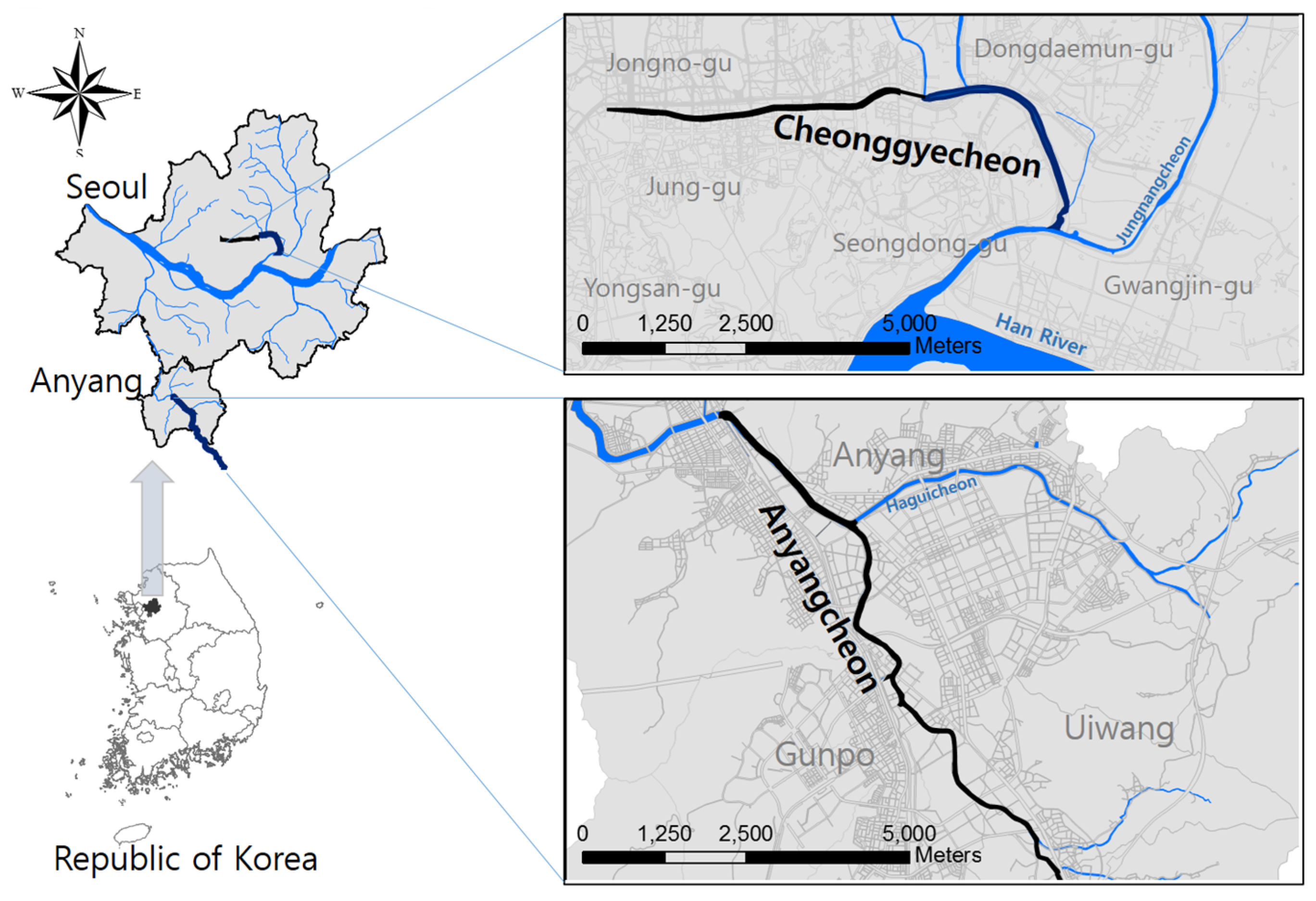
3.1. Study Area

Cheonggyecheon, which can be characterized as a city river, is one of the famous modern public recreation spaces in downtown Seoul, Korea. The length of this open stream is 10.92 km and its basin area is approximately 50.96 km², with over 6000 business buildings and more than 100,000 small individual shops, in one of the biggest commercial areas in Seoul. Historically, millions of people migrated to Seoul after the Korean War (1950–1953) and settled down along this stream with shabby makeshift houses. At this time, the accompanying garbage, waste, and deteriorating conditions became eyesores in Seoul. Hence, the stream was covered up with concrete and a 5.6-km-long, 16 m elevated expressway was constructed over the covered stream in the 1970s [26]. This urban structure and planning became an iconic example of the successful industrialization and modernization of Seoul until 2003. In July 2003, the mayor of Seoul, Lee Myung-bak (he later became the 17th president of the Republic of Korea), initiated the Cheonggyecheon Restoration Project to remove the elevated expressway and restore the surrounding environments of the stream. Due to the long period of neglect and economic development, Cheonggyecheon had been left nearly dry and had become the most traffic-congested area in the city. The main purposes of this project were to re-introduce nature to the city of Seoul, to promote an eco-friendly urban design, to restore the 30 years of lost history and culture of the region, and to revitalize the economy of the central business district of Seoul [27]. The Seoul Metropolitan Government initially budgeted 340 billion won (approximately US$254 million) to restore the stream by pumping fresh water from the Han River and to construct an artificial ecosystem in the stream. However, the final cost of the project was over 386 billion won (approximately US$281 million) in 2005 when the Seoul Metropolitan Government announced the reopening of Cheonggyecheon [28]. Due to its high cost and uncertain benefits, some researchers have criticized the success of the project and this debate has been moved on to the “Four Major Rivers Restoration Project”, which was initiated by the 17th president of the Republic of Korea, Lee Myung-bak. However, Lee and Anderson [29] concluded that the project improved the quality of life in Seoul and that the annual average visits to the restored stream numbered about 10 million with approximately 7.5 billion won for the annual maintenance cost. In addition, the Seoul Development Institute (SDI) [26] estimated the aggregated value of Cheonggyecheon restoration as over 356.2 billion won (approximately US$259 million).

In contrast to the Cheonggyecheon, Anyangcheon is an urban river running through four towns in Seoul and four cities Kyunggi Province. Approximately 3.87 million people reside in this watershed, with a population density of 13,500 persons per km². Primary land cover types within the watershed (as of 2000) comprise 43.03% urban area, 39.79% forest area, and 12.95% agricultural area [30]. Similar to most of the urban watersheds in Korea, the environmental quality of Anyangcheon, including the quantity and quality of the water, had degraded due to the negative externalities of rapid industrialization in Korea and resulted in devastating flood damage, stream depletion, and even the loss of biodiversity [31]. Due to these respects, the Seoul Metropolitan Government and the Anyang Municipal Government initiated the “Anyangcheon Ecological River Restoration Masterplan (2001–2013)” focused on ameliorating water quality, increasing water quantity, and restoring the ecosystem. The initial budget of this project was 49.6 billion won (approximately US$36.1 million). Unlike Cheonggyecheon, implementing this project resulted not only in increasing the number of biodiversity in ichthyofaunal, avifauna, and flora, but also in ameliorating the environment of the surrounding residential area by eliminating waste odor and providing better recreational facilities (e.g., a riverside bike road and waterfront areas). Kong, Park, and Yoo [32] concluded that the aggregated value of water quality improvement in this watershed can be estimated as approximately 83.0 to 109.7 billion won per year, which is approximately US$60.4 million to US$79.9 million. Figure 1 shows the location of the study areas.

The two studies (i.e., [26,32]) mentioned previously did not conduct the revealed preference approach to assess the value of environmental quality improvement due to the time of the research period. However, the revealed and stated preference approaches can be applied after the completion of projects to reassess whether the public investment is worthwhile.

3.2. Data

The individual travel data is required to estimate the consumer welfare in ecological river restoration projects. Among many recreational demands, we were particularly interested in the consumer welfare gain after heavily invested river restoration by the government. An on-site face-to-face interview survey was conducted for three weeks between 18 June and 24 July 2013 at Anyangcheon and Cheonggyecheon, simultaneously. To avoid survey bias, a sample survey (43 samples) was carried out before the main survey. Highly trained interviewers from a professional survey company conducted the interviews in an attempt to avoid interviewer bias. These interviewers targeted only adult respondents (i.e., age over 20) to obtain trip information including annual number of visits, travel time per visit, cost of travel and travel distance from their origin. The visitors’ characteristics were collected by demographic questions (i.e., income, dwelling type, age, gender, job, and education level). In this effort, 588 samples were collected from both sites. Based on the structured questionnaire, the means of the annual number of visits for Anyangcheon and Cheonggyecheon were 2.27 and 3.50, respectively, as shown in

Table 1. Mean of annual number of visits for study area.

Visit	Mean	Std. Err.	95% Conf. Interval
Anyangcheon	2.271	0.1197	2.035	2.506
Cheonggyecheon	3.507	0.2781	2.959	4.054

.

To calculate the travel cost associated with the opportunity cost endogenously, monthly income and travel time per visit were used. In order to convert monthly income into hourly income, monthly household income was divided by 640 (four households, eight hours per day, five days per week, four weeks per month). Direct travel cost and monthly household income were gained directly from the survey and the average travel cost per km was approximately $0.3. Thus, the travel cost used in the empirical model can be written as follows:

$$T{C}_i=\mathrm{Direct} \mathrm{Travel} {\text{Cost}}_i+T_i\times \frac{2}{3}\times \left(\mathrm{monthly} {\mathrm{Income}}_i/640\right)$$

(14)

where TC is the complete travel cost including the opportunity cost, $i$ is number of respondents, T is per-round-trip travel time from his/her origin.

Demographic questions were designed to capture the characteristics of visitors and the number of visits. Although the household income would be the major characteristic of the visitors, it was excluded in the empirical model due to the singularity problem from the aforementioned procedure of creating the TC. Variable names, definitions, and a summary of statistics are described in

Table 2. Variable names, definitions, and summary statistics.

Variables	Description	Anyangcheon Means	Cheonggyecheon Means
TC	Total round-trip travel cost associated with travel time opportunity cost (in US dollars)	16.72	15.08
		(0.54)	(1.28)
Gender	1 if survey respondent is male, 0 otherwise	0.493	0.479
		(0.030)	(0.030)
Job	1 if survey respondent is an office worker, 0 otherwise	0.264	0.250
		(0.026)	(0.026)
Education	Years of schooling	13.81	14.43
		(0.166)	(0.146)
Dwelling	1 if survey respondent lives in an apartment, 0 otherwise	0.750	0.559
		(0.026)	(0.029)
Age	Survey respondent’s age	45.81	40.57
		(0.878)	(0.895)
Income	Monthly household income (in US dollars)	3657.62	3972.85
		(55.69)	(89.55)

Note: Numbers in parentheses are standard errors and $1 equals ￦1105.

.

Visitors at Anyangcheon have slightly higher travel costs than those at Cheonggyecheon but the standard deviation of Cheonggyecheon is larger. It is assumed that the expected signs in terms of TC for both sites will be negative in the empirical results. The gender variable shows that more females than males visit Cheonggyecheon and their jobs are mostly office work. Unlike Cheonggyecheon, visitors at Anyangcheon are balanced in terms of gender variability but their job type is more of a managerial position. The sign for education is assumed to be positive for both sites as more educated individuals are willing to visit ecological restored sites in spite of travel costs. More visitors at Anyangcheon live in apartment-type homes than those at Cheonggyecheon. This result implies that individuals seeking a better environment visit more ecological restored sites. In addition, relatively younger people prefer to visit Cheonggyecheon due to its location. Therefore, the latter two statistics are expected to show negative and positive signs, respectively, in the empirical results.

4. Empirical Results

Table 3. Coefficients of the four selected models for Anyangcheon and Cheonggyecheon.

Variables	Anyangcheon				Cheonggyecheon
	Poisson	NB	ZTNB	TSNB	Poisson	NB	ZTNB	TSNB
Intercept	0.7034 *	0.6986 *	0.1800	−0.9354	1.287 *	1.249 *	0.9649	−14.10
	(0.4059)	(0.4513)	(0.7454)	−0.9354	(0.2612)	(0.4005)	(0.6070)	(553.63)
TC	−0.0181 *	−0.0180 *	−0.0339 *	−0.0358 *	−0.0306 *	−0.0200 *	−0.0523 *	−0.0532 *
	(4.43 × 10−6)	(4.82 × 10−6)	(8.19 × 10−6)	(8.27 × 10−6)	(3.15 × 10−6)	(3.60 × 10−6)	(7.76 × 10−6)	(7.46 × 10−6)
Gender	0.0672	0.0617	0.0984	0.1040	−0.0193	−0.0154	−0.0655	−0.0659
	(0.0859)	(0.0953)	(0.1549)	(0.1575)	(0.0626)	(0.1026)	(0.1626)	(0.1505)
Job	0.1520	0.1505	0.2290	0.2432	0.0842	0.0926	0.0677	0.0581
	(0.1001)	(0.1112)	(0.1809)	(0.1843)	(0.0848)	(0.1314)	(0.2090)	(0.1937)
Education	0.0091	0.0101	0.0232	0.0247	−0.0196	−0.0214	−0.0202	−0.0196
	(0.0188)	(0.0208)	(0.0337)	(0.0342)	(0.0139)	(0.0220)	(0.0330)	(0.0305)
Dwelling	0.0639	0.0602	0.0969	0.1012	−0.2465 *	−0.2101 *	−0.2599	−0.2596
	(0.0957)	(0.1057)	(0.1707)	(0.1735)	(0.0644)	(0.1065)	(0.1680)	(0.1555)
Age	−0.0041	−0.0039	−0.0064	−0.0068	0.0163 *	0.0157 *	0.0183 *	0.0178 *
	(0.0032)	(0.0035)	(0.0058)	(0.0059)	(0.0024)	(0.0037)	(0.0056)	(0.0052)
Income	0.00009 *	0.0180 *	1.45 × 10−4 *	1.53 × 10−4 *	1.76 × 10−5	−1.19 × 10−5	−1.14 × 10−5	−1.07 × 10−5
	(0.0000)	(0.0000)	(0.0000)	(0.0000)	(0.0000)	(0.0000)	(0.0000)	(0.0000)
# Obs.	288					300
LR chi2	30.56	19.99	28.15	29.72	325.83	94.47	93.95	104.28
Prob. > chi2	0.0001	0.0028	0.0002	0.0001	0.0000	0.0000	0.0000	0.0000
LL	−508.91	−500.89	−434.29	−432.11	−822.62	−660.20	−556.73	−557.33
Theta (θ)		0.0965	0.5236	1.487		0.4350	1.314	3.875
		(0.0316)	(0.1657)	(0.7152)		(0.0527)	(0.3518)	(0.0000)

Note: Numbers in parentheses are standard errors, and * indicates significance at the 5% level.

gives the estimation results for the four selected models, the Poisson, the negative binomial (NB), the zero-truncated negative binomial (ZTNB), and negative binomial model adjusted for both truncation and endogenous stratification (TSNB), of Anyangcheon and Cheonggyecheon. Before we analyze the results of the four models, the over-dispersion test was conducted by reporting the theta (θ) parameter for all negative binomial models. It is obvious that the collected data of both Anyangcheon and Cheonggyecheon have over-dispersion and thus there is a need to analyze the less-restricted models (i.e., NB, ZTNB, and TSNB). In addition, all NB, ZTNB, and TSNB models show significant levels of model fitness for both rivers.

In estimating the travel demand for ecological river restoration projects, all selected models for both Anyangcheon and Cheonggyecheon show significant negative signs for TC as expected. For the gender variables, male respondents are approximately 6.7%, 9.8%, and 10.4% more likely to visit Anyangcheon based on the less-restricted models. On the other hand, it can be observed that there is an approximately 1.5% to 6.5% decrease in travel demand for males in Cheonggyecheon. Visitors who have higher academic achievement tend to visit Anyangcheon more and Cheonggyecheon less based on the selected models. Likewise, visitors who live in apartments show similar results in academic achievement. However, visitors who have higher incomes tend to visit Anyangcheon more but not Cheonggyecheon. Furthermore, the older visitors tend to visit Cheonggyecheon more and office workers are more likely to visit both sites.

The individual travel cost method can be calculated and the individual consumer surplus (CS) of ecological river restoration can be estimated by using Equation (13). Empirical results from the travel cost associated with the opportunity cost in Table 3 and the mean of annual visits in Table 1 enable us to estimate the annual individual consumer surplus for Anyangcheon and Cheonggyecheon in

Table 4. Consumer surplus for Anyangcheon and Cheonggyecheon.

Site	Model	Annual CS	Value (US$)	p > $\mathbf{\left|}\mathit{Z}\mathbf{\right|}$	95% Conf. Interval
Anyangcheon	NB	/person	113.86	0.000	54.25	173.48
		/person/visit	50.14	0.000	23.89	76.39
		Total CS	100,280,000
	ZTNB	/person	60.57	0.000	31.93	89.22
		/person/visit	26.67	0.000	14.06	39.29
		Total CS	53,340,000
	TSNB	/person	57.40	0.000	31.40	83.39
		/person/visit	25.27	0.000	13.82	36.72
		Total CS	50,540,000
Cheonggyecheon	NB	/person	158.94	0.000	102.73	215.15
		/person/visit	45.32	0.000	29.29	61.35
		Total CS	453,200,000
	ZTNB	/person	60.71	0.000	43.04	78.39
		/person/visit	17.31	0.000	12.27	22.35
		Total CS	173,100,000
	TSNB	/person	59.65	0.000	43.26	76.03
		/person/visit	17.01	0.000	12.33	21.68
		Total CS	170,100,000

Note: $1 = ￦1105.

. Although all the selected models report statistically significant results in terms of individual annual consumer surplus, evidence of over-dispersion was observed through the likelihood ratio test. Therefore, a conventional way to correct this problem to estimate individual annual consumer surplus is to apply a better fitted model such as the negative binomial. Moreover, since the survey was specifically targeted for those who actually visited the study sites, the value zero cannot occur in the count data. In this sense, individual annual consumer surplus for both sites should be calculated by the estimates from the zero-truncated negative binomial (ZTNB); otherwise, those values will be exaggerated due to the underestimation of the standard error [33,34]. Finally, the non-visitor problem can be fixed by the truncated model, but the endogenous stratification issue still remains due to on-site data collection. Thus, the negative binomial model adjusted for both truncation and endogenous stratification (TSNB) should be applied [23].

Our estimated results indicate that corrected individual annual consumer surplus for Anyancheon and Cheonggyecheon is approximately $57 and $59, respectively. In addition, the estimated value of the annual individual CS per single visit is approximately $25 and 17$ for Anyangcheon and Cheonggyecheon, respectively, which indicates that Cheonggyecheon has approximately 68% less economic value than Anyangcheon. Based on previous literature (i.e., [29,32]), the annual average number of visitors for Cheonggyecheon and Anyangcheon is assumed to be 10 million and two million, respectively. Thus, aggregated consumer surplus of Cheonggyecheon and Anyangcheon can be expanded to approximately US$170.1 million and US$50.5 million, respectively. Compared to [26,32], aggregated recreation values of the two sites show less, but the value of Anyangcheon exceeds its cost while Cheonggyecheon does not.

5. Conclusions

Rapid economic growth has often aggravated services and goods provided by healthy and self-sustaining rivers. In Korea, a number of river basins have deteriorated not only in their hydrological conditions but also in their aesthetic ones. The government of Korea, however, has continued to stimulate the economy, ignoring the fact of environmental degradation until recently. To resolve such a vicious circle and move forward to a virtuous circle, the Seoul Metropolitan Government invested a public expenditure of 386 billion won (approximately US$281 million) at Cheonggyecheon and the Anyang Municipal Government along with Seoul implemented the “Anyangcheon Ecological River Restoration Masterplan” by investing a public expenditure of 49.6 billion won (approximately US$36.1 million). The purposes of those two projects are to ameliorate water quality, increase water quantity, and restore ecosystem services. Although many ex ante economic feasibility studies often concluded that the social welfare is always positive [35], ex post analysis may be needed for those sites to re-examine their benefits since they are built by public investment.

In this research, to reassess the consumer surplus of two distinct ecological river restoration projects in Korea, a conventional revealed preference approach of environmental quality improvement and the effectiveness of public investment on the revitalization of urban and city rivers has been studied using the individual travel cost method (ITCM). Count data was collected by an on-site face-to-face interview and recreation demands of those sites with respect to the number of visits were estimated. Although social benefits of the ecological river restoration project were assessed by a holistic approach, few studies have compared the revealed preference to the stated preference. We excluded the Poisson models in the analysis due to over-dispersion and truncated models were also not considered due to endogenous stratification, but the negative binomial model adjusted for both truncation and endogenous stratification (TSNB) was conducted, alternatively. The interaction between annual visits for the two sites and the travel cost associated with the opportunity cost indicates a statistically significant negative relationship in two selected models. Moreover, sociodemographic variables such as years of schooling, dwelling type, and age are statistically not significant, but those variables represent visitors’ characteristics which could be considerable proxies of the future plans for restoring rivers in Korea. The adjusted negative binomial model is selected to estimate consumer surplus on the two sites based on the comprehensive analysis of model goodness-of-fit tests and concludes that the consumer surplus per person per visit at the sites is approximately US$25.3 and US$17.0, respectively. These results indicate that the benefits of the Anyangcheon Ecological River Restoration Project are higher than those of Cheonggyecheon, while the total cost of the projects was opposite. However, the total recreation benefits of Cheonggyecheon and Anyangcheon are approximately US$170.1 million and US$55.5 million, respectively.

Previous literature indicated that the total costs of the Cheonggyecheon and Anyangcheon projects were US$281 million and US$36.1 million, respectively, and concluded that the used and non-used values of those rivers are approximately US$356.2 million and US$60.4 million, respectively. These results clearly indicated that both ecological river restoration projects have benefits for the public. Empirical results of this study, however, show that the benefits of Anyangcheon only exceed its cost, which leads us to have a second thought on the success of the Cheonggyecheon restoration project. Although these ex post analysis results can be criticized as the individual travel cost method cannot incorporate the non-used value of study sites, a rational conjecture can be induced that the total economic value of Cheonggyecheon might be exaggerated by the ex ante economic feasibility study. Apparently, one of the initial plans for the Cheonggyecheon restoration project was to provide second-degree fresh water to the center of the Seoul Metropolitan Area, but Cheonggyecheon has flowed artificially treated water instead of natural water after completion of the project. In this sense, since respondents of the ex ante analysis may have high expectations of the restoration, the total economic value of Cheonggyecheon could have been overestimated at the time the previous feasibility study was conducted. On the contrary, the Anyangcheon River Restoration Project followed the initial masterplan to restore the ecological stream itself. In this regard, there is high similarity between ex ante and ex post analysis results, even though the latter result mostly incorporates the used value of the stream.

The results of this study can be translated into several policy perspectives. Like river restoration projects, ex ante economic feasibility studies are a mandatory procedure to increase the effectiveness of public investment in huge construction projects. There has been, however, no single attempt to monitor its effectiveness via a feedback system once the huge construction projects are completed. As the result of this study illustrates, a gap between initial plans and actual implementation can decrease social benefits and lead to drastic inefficiency in public investment. Thus, we have to consider legally binding methods to construct a feedback system for public construction projects, especially for huge ones. Furthermore, a sound governance system will be a key ingredient to build a mutual confidence among stakeholders. Unfortunately, Korea does not have a strong foundation for both systems which can be the cause of the incurring inefficiency in public investments not only in Cheonggyecheon but also in the other national-level huge construction projects such as the “Four Major Rivers Restoration Project”. Although this research tackles a gap between ex ante economic feasibility studies and ex post analysis using some economic valuation tools, a couple of limitations can be addressed for the future discussion. It is plausible that the direct and indirect methods should be considered to analyze the impacts of such a huge project. From the statistical point of view, a substitute site approach can improve the accuracy of indirect impacts which we ignored in this research due to the lack of information.

References

1. Postel, S.; Richter, B. Rivers for Life: Managing Water for People and Nature; Island Press: Washington, DC, USA, 2008. [Google Scholar]
2. Young, R.A.; Loomis, J.B. Determining the Economic Value of Water: Concepts and Methods; Routledge: London, UK, 2014. [Google Scholar]
3. Henry, C.P.; Amoros, C.; Roset, N. Restoration ecology of riverine wetlands: A 5-year post-operation survey on the Rhone River, France. Ecol. Eng. 2002, 18, 543–554. [Google Scholar] [CrossRef]
4. Ormerod, S.J. Restoration in applied ecology: Editor’s introduction. J. Appl. Ecol. 2003, 40, 44–50. [Google Scholar] [CrossRef]
5. Palmer, M.A.; Bernhardt, E.S.; Allan, J.D.; Lake, P.S.; Alexander, G.; Brooks, S.; Carr, J.; Clayton, S.; Dahm, C.N.; Shah, J.F.; et al. Standards for ecologically successful river restoration. J. Appl. Ecol. 2005, 42, 208–217. [Google Scholar] [CrossRef]
6. Malakoff, D. Profile—Dave rosgen—The river doctor. Science 2004, 305, 937–939. [Google Scholar] [CrossRef] [PubMed]
7. Beechie, T.; Pess, G.; Roni, P. Setting river restoration priorities: A review of approaches and a general protocol for identifying and prioritizing actions. N. Am. J. Fish. Manag. 2008, 28, 891–905. [Google Scholar] [CrossRef]
8. Johansson, M.E.; Nilsson, C. Responses of riparian plants to flooding in free-flowing and regulated boreal rivers: An experimental study. J. Appl. Ecol. 2002, 39, 971–986. [Google Scholar] [CrossRef]
9. Loomis, J.B.; Walsh, R.G. Recreation Economic Decisions: Comparing Benefits and Costs, 2nd ed.; Venture Publishing Inc.: State College, PA, USA, 1997. [Google Scholar]
10. Loomis, J. Quantifying recreation use values from removing dams and restoring free-flowing rivers: A contingent behavior travel cost demand model for the lower Snake River. Water Resour. Res. 2002. [Google Scholar] [CrossRef]
11. Timmins, C.; Murdock, J. A revealed preference approach to the measurement of congestion in travel cost models. J. Environ. Econ. Manag. 2007, 53, 230–249. [Google Scholar] [CrossRef]
12. Amoako-Tuffour, J.; Martinez-Espineira, R. Leisure and the net opportunity cost of travel time in recreation demand analysis: An application to gros morne national park. J. Appl. Econ. 2012, 15, 25–49. [Google Scholar] [CrossRef]
13. Rolfe, J.; Dyack, B. Valuing recreation in the coorong, australia, with travel cost and contingent behaviour models. Econ. Rec. 2011, 87, 282–293. [Google Scholar] [CrossRef]
14. El-Bekkay, M.; Moukrim, A.I.; Benchakroun, F. An economic assessment of the Ramsar site of Massa (Morocco) with travel cost and contingent valuation methods. Afr. J. Environ. Sci. Technol. 2013, 7, 441–447. [Google Scholar]
15. Bockstael, N.E.; McConnell, K.E. Environmental and Resource Valuation with Revealed Preferences: A Theoretical Guide to Empirical Models; Springer Netherlands: Dordrecht, The Netherlands, 2007. [Google Scholar]
16. Melstrom, R.T.; Lupi, F.; Esselman, P.C.; Stevenson, R.J. Valuing recreational fishing quality at rivers and streams. Water Resour. Res. 2015, 51, 140–150. [Google Scholar] [CrossRef]
17. Freeman, A.M. The Measurement of Environmental and Resource Values: Theory and Methods; Resources for the Future: Washington, DC, USA, 1993. [Google Scholar]
18. Kolstad, C.D. Environmental Economics; Oxford University Press: New York, NY, USA, 2000. [Google Scholar]
19. Braden, J.B.; Kolstad, C.D. Measuring the Demand for Environmental Quality; Elsevier Science Pub. Co.: North-Holland, The Netherlands, 1991. [Google Scholar]
20. Greene, W.H. Econometric Analysis, 6th ed.; Prentice Hall: Upper Saddle River, NJ, USA, 2008. [Google Scholar]
21. Cameron, A.C.; Trivedi, P.K. Econometric models based on count data. Comparisons and applications of some estimators and tests. J. Appl. Econ. 1986, 1, 29–53. [Google Scholar] [CrossRef]
22. Haab, T.C.; McConnell, K.E. Valuing Environmental and Natural Resources: The Econometrics of Non-Market Valuation; Edward Elgar Publishing: Cheltenham, UK, 2002. [Google Scholar]
23. Shaw, D. On-site samples regression: Problems of non-negative integers, truncation, and endogenous stratification. J. Econ. 1988, 37, 211–223. [Google Scholar] [CrossRef]
24. Englin, J.; Shonkwiler, J. Modeling Recreation Demand in the Presence of Unobservable Travel Cost: Toward a Travel Price Model. J. Environ. Econ. Manag. 1995, 29, 368–377. [Google Scholar] [CrossRef]
25. Hellerstein, D.; Mendelsohn, R. A theoretical foundation for count data models. Am. J. Agric. Econ. 1993, 75, 604–611. [Google Scholar] [CrossRef] [Green Version]
26. Seoul Development Institute (SDI). Feasibility Study and Master Plan of Cheonggyecheon Restoration: Mid-term Report; Seoul Development Institute: Seoul, Korea, 2003. [Google Scholar]
27. Hwang, K.Y. Restoring Cheonggyecheon Stream in the Downtown Seoul; Seoul Development Institute: Seoul, Korea, 2004. [Google Scholar]
28. Cho, M.R. The politics of urban nature restoration the case of cheonggyecheon restoration in Seoul, Korea. Int. Dev. Plan. Rev. 2010, 32, 145–165. [Google Scholar] [CrossRef]
29. Lee, J.Y.; Anderson, C.D. The restored cheonggyecheon and the quality of life in Seoul. J. Urban Technol. 2013, 20, 3–22. [Google Scholar] [CrossRef]
30. Chung, E.-S.; Lee, K.S. Identification of spatial ranking of hydrological vulnerability using multi-criteria decision making techniques: Case study of Korea. Water Resour. Manag. 2009, 23, 2395–2416. [Google Scholar] [CrossRef]
31. Kim, Y.; Chung, E.-S.; Jun, S.-M.; Kim, S.U. Prioritizing the best sites for treated wastewater instream use in an urban watershed using fuzzy topsis. Resour. Conserv. Recycl. 2013, 73, 23–32. [Google Scholar] [CrossRef]
32. Kong, K.; Park, D.H.; Yoo, J.C. Estimating of social preference of the watershed resident about the anyangcheon watershed water quality improvement. J. Korea Water Resour. Assoc. 2008, 41, 315–324. [Google Scholar] [CrossRef]
33. Ismail, N.; Jemain, A.A. Handling overdispersion with negative binomial and generalized Poisson regression models. In Casualty Actuarial Society Forum. Winter 2007. Including the Ratemaking Call Papers; Casualty Actuarial Society: Arlington, VA, USA, 2007; pp. 103–158. [Google Scholar]
34. Sileshi, G. Selecting the right statistical model for analysis of insect count data by using information theoretic measures. Bull. Entomol. Res. 2006, 96, 479–488. [Google Scholar]
35. Lee, Y.; Chang, H.; Hong, Y. Is a costly river restoration project beneficial to the public? Empirical evidence from the Republic of Korea. Desalination Water Treat. 2015, 54, 3696–3703. [Google Scholar] [CrossRef]
Figure 1. Study area.
Sustainability 08 00353 g001