Article

Input vs. Output Taxation—A DSGE Approach to Modelling Resource Decoupling

by
Marek Antosiewicz
1,2,*,
Piotr Lewandowski
1 and
Jan Witajewski-Baltvilks
1
1
Institute for Structural Research, Warsaw 02-516, Poland
2
Warsaw School of Economics, Warsaw 02-554, Poland
*
Author to whom correspondence should be addressed.
Sustainability 2016, 8(4), 352; https://doi.org/10.3390/su8040352
Submission received: 8 February 2016 / Revised: 1 April 2016 / Accepted: 5 April 2016 / Published: 12 April 2016

Abstract

:
Environmental taxes constitute a crucial instrument aimed at reducing resource use through lower production losses, resource-leaner products, and more resource-efficient production processes. In this paper we focus on material use and apply a multi-sector dynamic stochastic general equilibrium (DSGE) model to study two types of taxation: tax on material inputs used by industry, energy, construction, and transport sectors, and tax on output of these sectors. We allow for endogenous adoption of resource-saving technologies. We calibrate the model for the EU27 area using an IO matrix. We consider taxation introduced from 2021 and simulate its impact until 2050. We compare the taxes along their ability to induce reduction in material use and raise revenue. We also consider the effect of spending this revenue on reduction of labour taxation. We find that input and output taxation create contrasting incentives and have opposite effects on resource efficiency. The material input tax induces investment in efficiency-improving technology which, in the long term, results in GDP and employment by 15%–20% higher than in the case of a comparable output tax. We also find that using revenues to reduce taxes on labour has stronger beneficial effects for the input tax.

1. Introduction

The need to limit the use of natural resources is becoming one of the most pressing issues for policy-makers. On the one hand, exhaustive use of resources, which are available only in limited supply, can potentially limit the production possibilities and welfare of future generations. On the other hand, use of resources such as fossil fuels increases air pollution and releases carbon to the atmosphere causing the greenhouse effect. The importance of the problem has been recognized by, among others, policy-makers in the European Union [1], United States [2], and China in its 12th five-year plan for years 2011–2015 [3].
There are several policy options for resolving the problem of excessive resource use. If one thinks that today’s production puts a burden on future generations, a tax on today’s output constitutes a solution. If one thinks that the current market prices of resources do not reflect their true social costs (e.g., due to atmospheric pollution), then a tax on inputs [4] constitutes a solution. Other options include performance standards, which require firms to limit the use of resources per unit of output and incentivize firms to adopt more efficient technologies, or R&D and deployment subsidies, which support development and adoption of cleaner technologies. In this paper we limit our attention to the first two policy options: a tax on input and a tax on output.
An input tax is a popular policy instrument for achieving fiscal and environmental goals. The most common example of this tax is the petroleum tax. In our study we examine the consequences of replacing this tax with a hypothetical tax on outputs of the most resource- and pollution-intensive industries, such as the cement, natural fertilizers, or electronic equipment industry. Using the classification of material and resource taxes proposed in [4], the input tax falls into the category of taxation of materials when they enter into production, and the output tax as a tax levied on resource-intensive final products.
We use a multi-sector dynamic stochastic general equilibrium (DSGE) model of the EU27 area to simulate the impact of these taxes levied on industry, energy, construction, and transport sectors. We allow for endogenous investment in resource-efficiency improvement and account for labour market adjustments. We find that input and output taxation create contrasting incentives and have an opposite effect on resource efficiency, which implies different dynamics of material use and macroeconomic outcomes. Simulating tax rates which lead to an equal drop in material use, we find that the material input tax results in GDP and employment that is 15%–20% higher compared to the scenario with the output tax. Simulating tax rates that equate the tax revenue, we find that the output tax results in a much smaller drop in material use. Additionally, we find that using the tax revenue to reduce labour taxation is much more efficient in the case of input tax. Thus, the input tax implies smaller macroeconomic costs and better resource efficiency outcomes than the output tax in all variants of the simulations considered. This leads us to the conclusion that a material input tax is a more efficient instrument to achieve resource decoupling.
In the paper we highlight and discuss one reason for the different effects of input and output tax: a material tax provides an incentive for firms to substitute materials with material-saving technologies. Thus, a given reduction in material use is associated with a smaller reduction in production. Indeed, as we demonstrate in the sensitivity analysis, larger substitutability between materials and material-saving technologies is associated with lower GDP loss upon introduction of a material tax.
The ability of technology to substitute for the use of resources and energy has been documented in a range of empirical studies. For example, in [5] it is shown that an energy-related patent, on average, leads to long-run energy savings worth $14.5 million (median present value of long run energy-savings from nine industries in which savings were observed: automotive, chemicals, copper, electrometallurgical, iron foundries, plastic film and sheet, pulp and paper, and steel pipes and tubes). Sue Wing [6] uses industrial data on factor use and patent data to decompose changes in the US energy intensity by industries into changes in industrial composition, factor substitution, technological change induced by changes in energy prices, and the disembodied technological change. He finds that induced technological change leads to energy savings, although its contribution is small relative to the other factors in the decomposition. Fæhn et al. [7] finds that a 10% increase in the energy price leads to technology adoption that results in a 1% lower energy demand by new firms.
The paper contributes to the literature on the effectiveness of various policies aimed at the reduction of resource and material use. There are numerous theoretical studies which examine the optimal policy mix for reduction in the use of fossil fuels. Popp [8] and Fischer et al. [9] find that a combination of carbon tax with R&D subsidies promoting efficient technologies brings more benefit than any of the single policies. Gerlach and van der Zwaan [10] highlight the role of efficiency standards, which, as they argue, promote lower fuel consumption, as well as adoption and development of more efficient technologies. More recently, the literature was extended by studies which analyse policies promoting material efficiency. Soderholm and Tilton [11] argue that policies should correct the externalities directly but should not set any targets for material efficiencies, as it is not clear what material efficiency target is socially optimal. In response to this argument, Allwood et al. [12] replied that although material efficiency may not be optimal from the economic perspective, it is going to face less political and social resistance than e.g., a carbon tax. Skelton and Allwood [13] examined the impact of carbon prices on efficiency in the use of steel. They find that substitution possibilities between material and labour matters for the policy effects. We extend the analysis of [13] by allowing for general equilibrium effects (e.g., adjustment of wages to changes in unemployment).
In contrast to the above papers, our paper does not suggest what the optimal policy mix is, but rather highlights what effects determine the success of the input tax when compared to the output tax. We extend the literature by analysing the impact of taxes not only on costs of policies in terms of GDP, but also in terms of employment.
In addition, the paper verifies whether the macroeconomic performance of both taxes changes under the alternative uses of tax revenue—reducing taxation on labour instead of transferring it to household. The importance of tax recycling has been evidenced by the literature on the double dividend hypothesis, which states that the cost of climate policies can be reduced if the revenue from taxes and fees on emissions is used to decrease other distortionary taxes. The authors in [14] and [15] demonstrated that models need to take into account the presence of non-environmental distortionary taxes in order to accurately assess the macroeconomic performance of environmental taxes. There are also studies which find support for the hypothesis by comparing the effects of various tax recycling at a national level (e.g., [16,17]).
In the next section we present our macroeconomic DSGE model which allows for endogenous adoption of material-saving technologies. We discuss the calibration of the model for the EU27 area, using an Input Output matrix and literature findings. We lay out a simulation strategy for taxation introduced from 2021. Although all model variables are simulated, we focus on taxation impacts on GDP, national accounts, labour market, resource use, and public finances until 2050. In the third section, we present our results. Firstly, we compare the impact of input and output taxes which lead to the same total reduction in resource use in 2050. Secondly, we compare the impact of input and output taxes which raise the same revenue in 2050. Next, we check how sensitive the results are to the alternative uses of tax revenue. Lastly, we conduct a sensitivity analysis and examine how our results change when we vary the parameter determining the substitutability between materials and material-saving technologies. In the final section we discuss our findings.

2. Materials and Methods

In this section we describe the model and the simulation setup. Regarding the model description, we specify the production structure of firms, which is crucial for the modelling of a firm’s response to input and output taxation, and is the focus of the paper. A detailed description of the remaining agents of the model and the solution method can be found in [18], and a summary of variables and parameters which are discussed in this section can be found in Table A1 in Appendix A.

2.1. Model Description

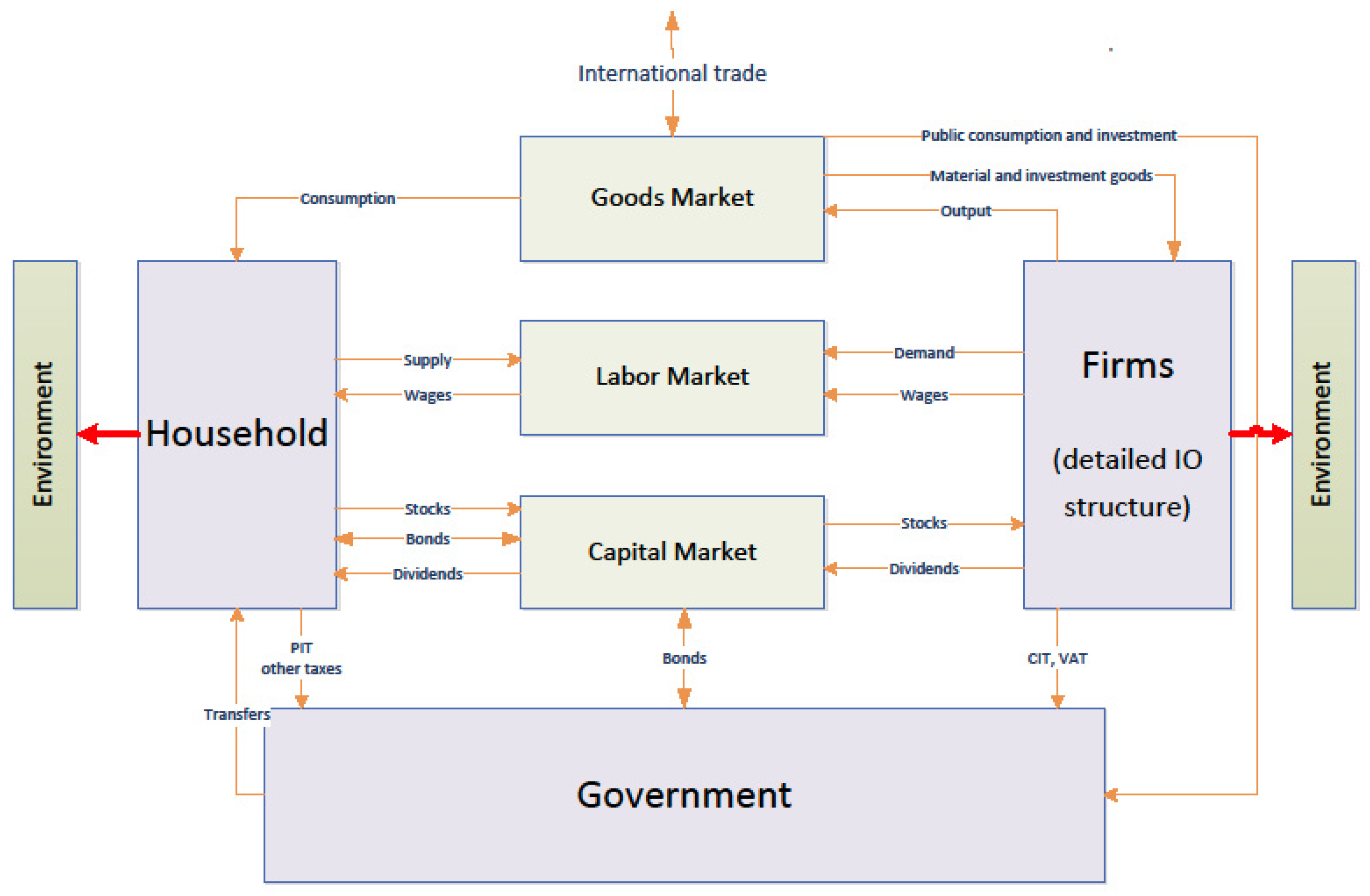
We use a multi-sector, large-scale dynamic stochastic general equilibrium (DSGE) model which we calibrate and estimate for the EU27 area (we calibrate our model to Eurostat Input Output tables and Eurostat only provides them for the EU27 area, which consists of all the current member states except for Croatia). The main economic agents in the model are: households, representative firms in each of the eight sectors and government. The basic scheme of the model is shown in Figure 1.
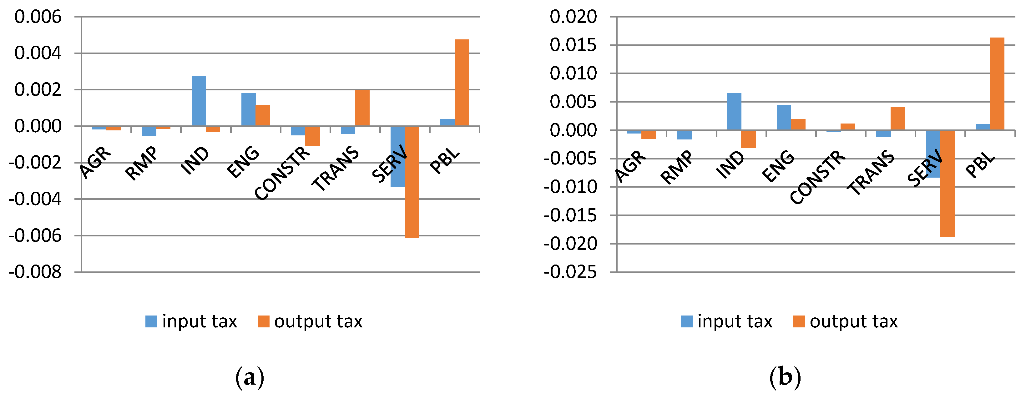
The model is disaggregated into the following sectors: Agriculture (AGR), Raw Material Production (RMP), Industry (IND), Energy (ENG), Construction (CONSTR), Transport (TRANS), Market Services (SERV) and Public Services (PBL). Table 1 summarizes the sector structure of the model.
In each sector s S a representative firm maximises the expected, discounted profits:
max E   t = 0 Λ t Π t s
where Λ t is the stochastic discount factor mirroring the preferences of the household and Π t s are the profits of the firm. The firm operates a multi-stage production technology using CES functions. In the first stage, capital K t s is combined with energy intermediate material E N G t s in order to produce composite good K E t s :
K E t s = [ ( 1 θ E s ) ( K t s ) ϵ E s 1 ϵ E s +   θ E s ( E N G t s ) ϵ E s 1 ϵ E s ] ϵ E s ϵ E s 1
where θ E s is a parameter determining the share of energy in the composite good and ϵ E s denotes the firm’s short-term elasticity of substitution between capital and energy. In the second stage the composite good K E t s is combined with labour N t s in order to produce another composite good:
K L E t s = [ θ K E s ( K E t s ) ϵ K E s 1 ϵ K E s + ( 1 θ K E s )   ( N t s ) ϵ K E s 1 ϵ K E s ] ϵ K E s ϵ K E s 1
where parameter θ K E s sets the shares of the production factors, and ϵ K E s sets the firm’s short-term elasticity of substitution. In the final stage of production, the second composite good is combined with material good M t s :
Y t s = [ ( 1 θ M s ) ( K L E t s ) ϵ M s 1 ϵ M s +   θ M s ( M t S ) ϵ M s 1 ϵ M s ] ϵ M s ϵ M s 1
where θ M s is the share parameter of the production factors and ϵ M s sets the firm’s short-term elasticity of substitution between materials and other factors of production.
Aggregate intermediate material is produced using goods from all sectors of the model in a two-step procedure. Since we are mainly interested in assessing effects of policies on the Materials Production sector (A02 and B in Eurostat CPA) we proceed with the following approach. We assume that material good is composed of a material good of the Raw Material Production sector M t s , R M P and a bundle of goods from remaining sectors M O t s with a CES function, which also accommodates endogenous material efficiency. Then, the bundle of remaining material goods is produced using Leontief function. This can be summarized in the following equations:
M t s = [ E F F t s θ R M P s ( M t s , R M P ) ϵ R M P s 1 ϵ R M P s + ( 1 θ R M P s )   ( M O t s ) ϵ R M P s 1 ϵ R M P s ] ϵ R M P s ϵ R M P s 1
u S   M t s , u = θ u s M O t s
As usual, θ R M P s and ϵ R M P s set the share and short-term elasticity in the CES composite, whereas parameters θ u s set the share of material good of sector u in the production function of sector s . The variable E F F t s sets the material efficiency of sector s and, in the steady state, it is normalised to unity. Each intermediate material use variable M t s , u is a composite of home and foreign produced goods, which are additionally denoted by subscripts H and F:
M t s , u = [ θ H s , u ( M t , H s , u ) ϵ H s 1 ϵ H s + ( 1 θ H s , u )   ( M t , F s , u ) ϵ H s 1 ϵ H s ] ϵ H s ϵ H s 1
Endogeneity of technology choices means that firms are allowed to change the characteristics of technology parameters of production function under market incentives. For instance, an increase in energy prices incentivizes the firm to invest in the more costly, energy-saving technology. Effectively, this gives firms the possibility to substitute inputs with capital. Importantly, these substitution possibilities are limited in the short-run: we assume that the efficiency of technology is the weighted average between past and today’s technology choices. In particular, we let E F F t s be determined by:
E F F t s = E F F t 1 s ( 1 δ ) K t 1 s K t s + Z t s I t s K t s
where K t s is the stock of capital, I t s is the level of investment and Z t s is the firm’s choice of technology at time t . More efficient technology involves higher cost of capital goods. Specifically, the cost of capital goods is given by:
I C t s = I t s ( 1 + ( c Z t s ) α )
Parameter α sets the degree of rigidity with respect to changes in technology and implicitly sets the medium- and long-term elasticity of substitution between materials and remaining inputs. Note that if α = , firms always choose Z = 1 .
The profit of the firm is given by the revenue from sales of good Y t s less the cost of labour, investment, intermediate materials, vacancy posting, and taxes. Goods produced by the sector firms are aggregated by final goods firms, which produce consumption, public, investment, and export goods. The final goods production structure is given by the Input-Output matrix.
The consumer maximises utility from consumption subject to her income which is composed of labour income less taxes, dividends from firms, and transfers from the government. The government collects labour, VAT, and environmental taxes and spends it on the purchase of the public good and on transfers to the household. The labour market is modelled according to the search and matching framework, similar to [19,20]. The unemployment rate is determined endogenously and depends on the number of vacancies generated by firms, and the intensity of job search by job seekers. The decisions of firms on the opening of vacancies depends on the current and future states of the economy. The key macroeconomic assumption of the DSGE model is that the economy is on the balanced growth path at the beginning of the time horizon and that it will continue on this path if no policies are introduced.
The sector structure of the model is calibrated using the NACE Rev. 2 Input-Output matrices for the year 2010 available from Eurostat. The flows are determined by the share parameters θ which appear in equations determining the production structure. The elasticity parameters are set as follows:
  • ϵ E s —short-run elasticity between capital and energy in the production function of a firm. According to numerous studies, the elasticity of substitution between these factors is very low [21,22]. We set this parameter at 0.1.
  • ϵ K E s —short-run elasticity between capital-energy composite and labour in the production function of a firm. The standard practice of DSGE models is to use the Cobb–Douglas specification, e.g. [23], which implies a value of 1. We set this parameter to a value of 0.95, i.e., lower than unity. This is motivated by the recent study in [24], which shows that sector-specific elasticity estimates are significantly below unity.
  • ϵ M s —short-run elasticity between capital-energy-labour composite and materials in the production function of a firm. We set this elasticity at 0.3 following the CGE model in [25].
  • ϵ R M P s —short-run elasticity between RMP material and other materials in the production function of a firm. A study in [26] shows that the elasticity of substitution between fuels and other raw materials goods is low. We also set a small value of 0.1, although the RMP sector includes other materials apart from fuels.
  • ϵ H s —short-run elasticity between home and foreign goods in the production function of a firm. The literature regarding this elasticity shows that it can take a wide range of plausible values. For example, in a study [27] it is estimated that for the G7 countries this elasticity is in the range between 0.1 and 2. Heathcote and Perri [28] demonstrated that low values of this parameter result in a model that better reproduces business cycle properties of data. We set this value at 0.4.

2.2. Simulation Setup

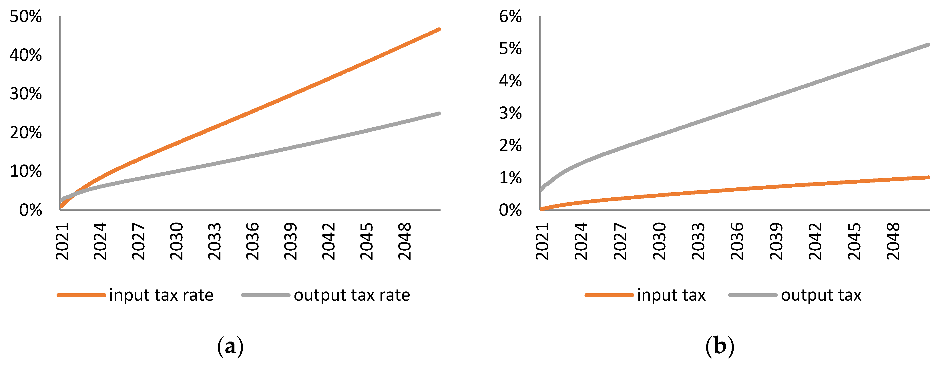
We use the model described in the previous subsection to compare the two tax schemes in their ability to reduce material use and their economic impact, measured among others in output, employment or sector shifts in the economy. We define the input tax as an excise-type tax on the purchase of the intermediate materials of the Raw Material Production sector by the Industry, Energy, Construction, and Transport sectors. We define the output tax as an excise (non-deductible) tax which is levied on the value added generated by these four sectors.
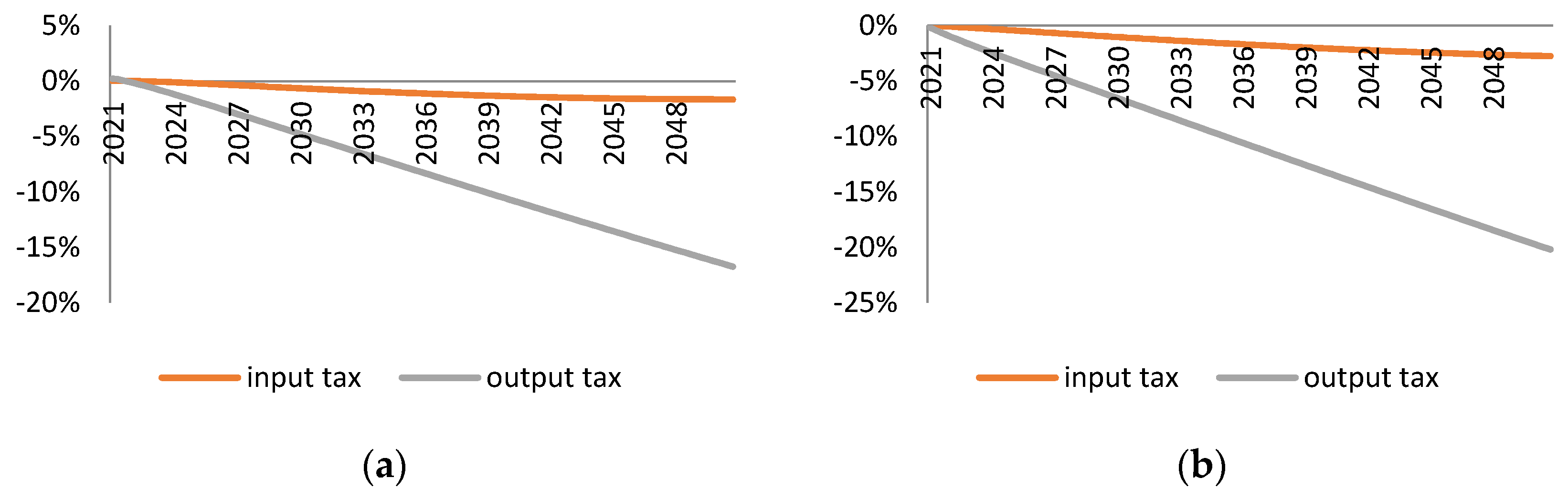
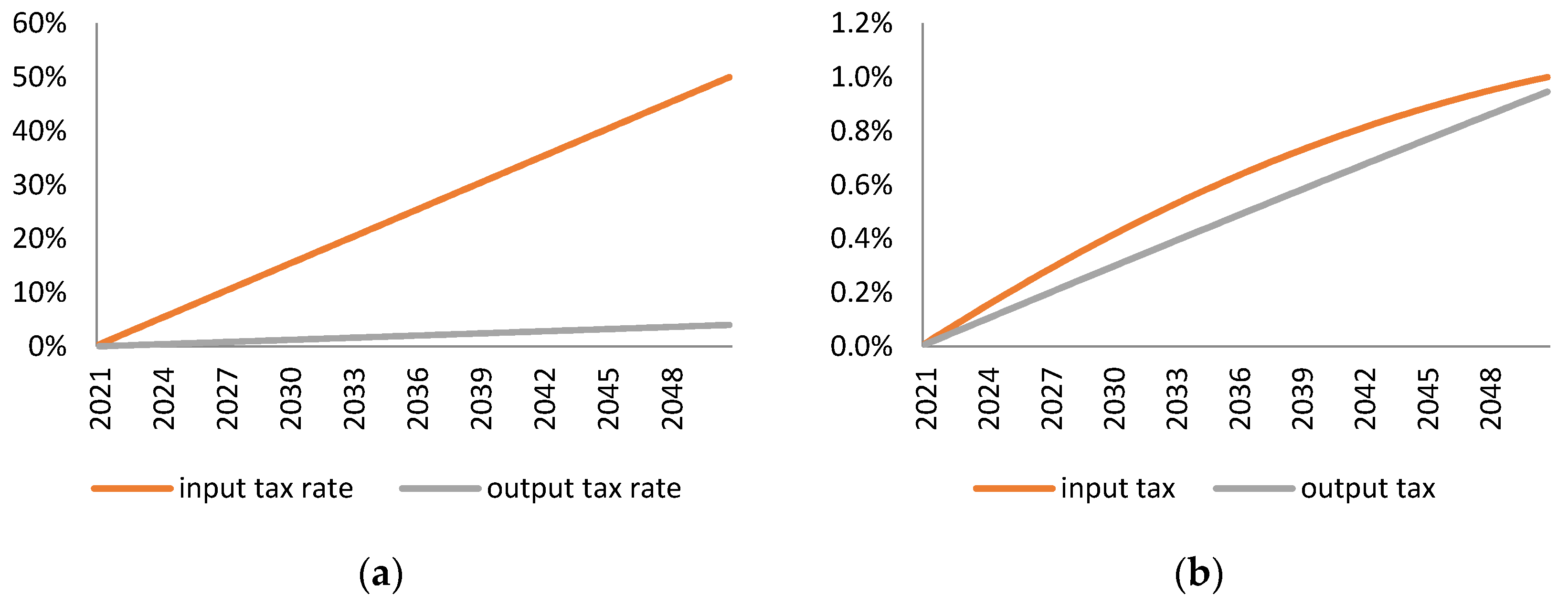
In order to assess the taxes along a possibly wide range of dimensions, we perform several simulation experiments. In the basic experiment we consider two simulations which differ in the basis for the comparison of the two taxes. In the first simulation we follow a material reduction approach. For each type of tax we simulate such a (roughly linear) path of tax rates that the resulting decrease of the RMP sector output gradually (linearly) reaches 20% in 2050 (from 0% in 2021). The start date is set in order to make the study relevant for the current debate on EU environmental policies. On the other hand, given that the target in our simulations is ambitious, we let the policies be introduced gradually until 2050. In the second simulation we follow a fiscal approach. For each type of tax we simulate such a linear path of tax rates that the revenue in 2050 reaches approximately 1% of GDP. For both of these simulations we assume that the revenues are used as a lump sum transfer to the household. Such fiscal closure allows us to analyse only the price incentives that the tax has for the behaviour of firms.
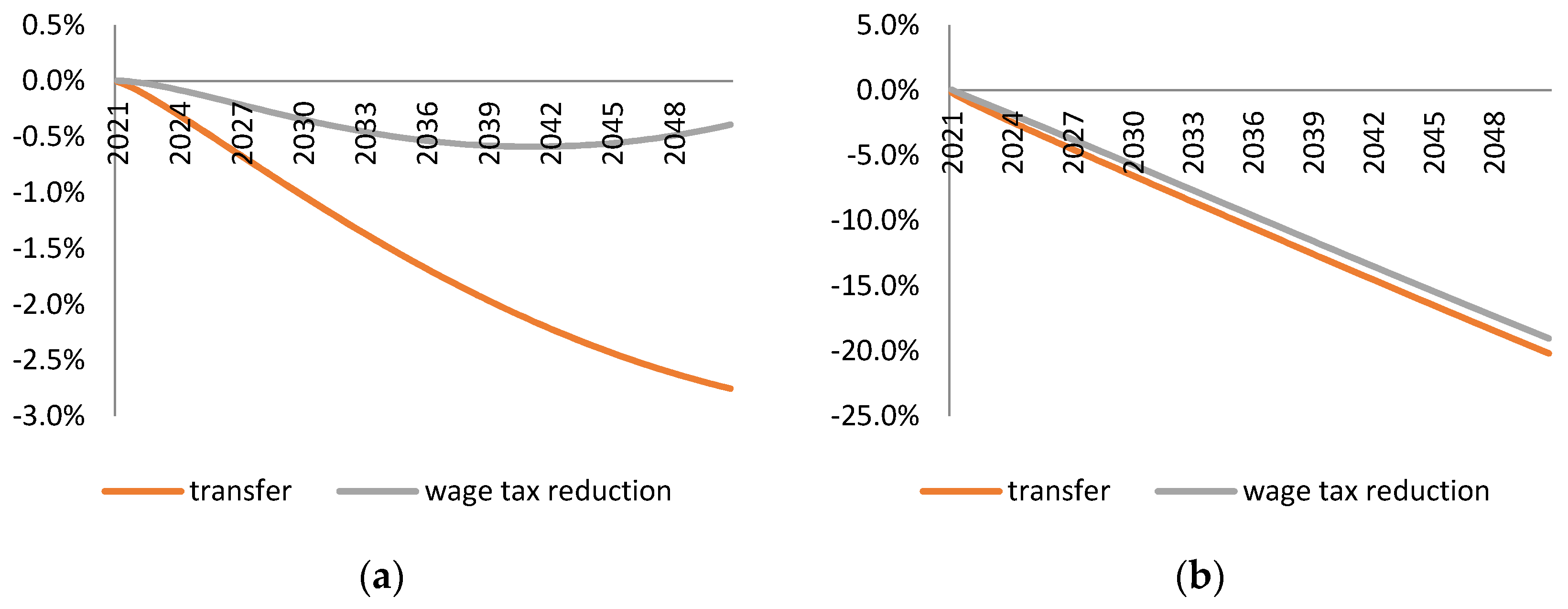
In the third simulation experiment we modify the fiscal closure. We follow the first simulation setup (material reduction approach) but we assume that 20% of the tax revenue is spent on lowering labour taxation. The main aim of this simulation is to compensate for the fact that the two taxes differ significantly in the total revenue they generate (higher in the case of the output tax). The offsetting effect of lower labour tax reduction will, therefore, be stronger in the case of the output tax.
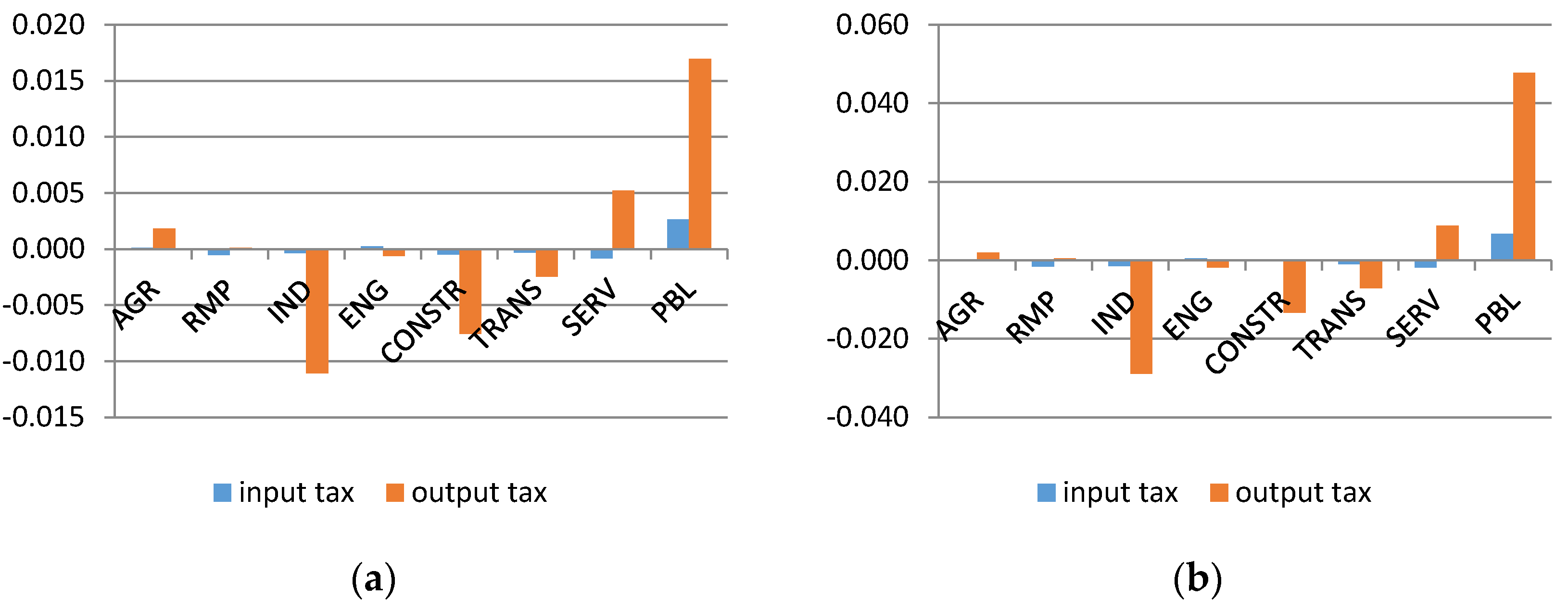
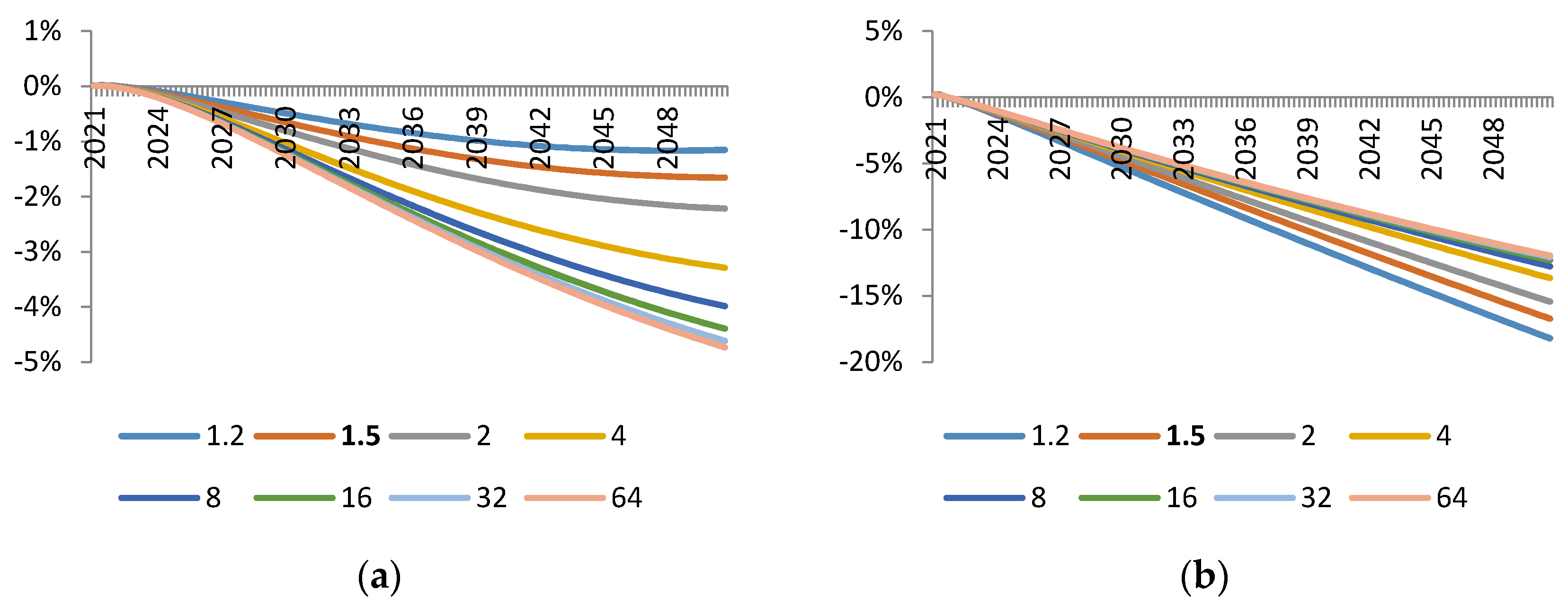
Lastly, we check the robustness of our results. Due to the fact that the results depend, to a large extent, on the endogenous material efficiency mechanism, we perform a sensitivity analysis with respect to the elasticity parameter which governs this mechanism. Again, we follow the material reduction approach as in the first simulation exercise. All simulations are performed using the Kalman filter [18]. Results are expressed as deviations from the steady state of the model, which we interpret as the baseline growth scenario for the EU27.

3. Discussion of Results

3.1. Equalling Material Reduction

This subsection shows results for the first simulation approach in which we set tax rates as to achieve a material reduction of 20% at the end of the simulation horizon (2050). We start with discussing the basic macroeconomic impact of the two taxes as measured by the response of gross domestic product, employment, investment, and imports, which is shown in Figure 2. Both taxes have a negative impact on all economic indicators; however, the output tax causes a much stronger decline. The drop in GDP in 2050 is equal to 16.7% for the output tax, against 1.7% for the input tax. This is equivalent to a reduction of the yearly growth rate by 0.6 and 0.06 percentage points, respectively, between 2021 and 2050. For both taxes the impact on employment and investment is slightly stronger than on GDP: for the output tax it amounts to 20.2% and 26.7% in 2050, respectively, whereas for the input tax to 2.8% and 3.6%, respectively. The decrease in international trade, measured by value of imports is most pronounced (the drop in exports is roughly the same as in imports for both taxes, leaving the current account stable), leading to a more closed European economy—the drop is equal to 31.1% and 10.6% for the output and input tax, respectively, which is much stronger than the impact on GDP. It has to be noted, however, that the foreign trade in the model is the trade of the EU27 area with the rest of the world. It does not take into account trade between the EU member states. The relative impact on trade (relatively to GDP deviation) is much stronger in the case of the input tax, because the input tax directly taxes imports of material goods, as opposed to the output tax, which decreases the competitiveness of home-produced vs. foreign goods.
Figure 3a shows the endogenously calculated tax rates which are necessary for achieving the assumed decrease of the output of the material production sector. Both tax rates increase roughly linearly from 2021 and, in 2050, reach approximately 47% for the input tax and 25% for the output tax. However, Figure 2b shows that the output tax generates much higher revenue—it reaches 5% of baseline GDP in 2050 (6% of GDP if we take into account the endogenous fall of GDP resulting from the tax), which is slightly less than the revenue from value added tax in the European Union (according to Eurostat, 7% of GDP in 2014). Hence, we believe that the output tax should be treated not only as a measure aimed at reducing material use, but also as a source of additional, considerable tax revenue. The difference in total tax revenue generated by both taxes is mainly due to the size of the base on which they are levied—for the input tax it is approximately 3% of GDP; for the output tax— approximately 25% of GDP. Moreover, we find that the endogenous reduction of the tax base is considerably stronger in the case of the input tax.
However, the crucial difference between the two taxes is in the endogenous response of firms concerning investment in material efficiency. Figure 4 shows effects of both taxes on investment in material efficiency in sectors on which the tax is levied (Industry, Energy, Construction, Transport). The input tax, which increases the price of intermediate material input in the production function, induces offsetting additional firm investment in technology. Our model shows that in 2050, firms operating in these sectors are able to produce approximately 15% more output from a unit of RMP intermediate material. In the case of an output tax, the price signal works in the opposite direction. Firms do not see a direct link between the tax and their material efficiency and, therefore, invest less in cleaner, more resource-efficient technologies. Due to the limited substitution possibilities between material input and other factors of production, the final outcome is a strong GDP contraction as reported in Figure 2.
Now we discuss adjustments in the sector structure of GDP and employment, as well as the potential of shifting towards a more service-based economy as a result of taxation aimed at resource decoupling. Figure 5 and Figure 6 show the impact of both taxes on the sector structure of GDP and employment in 2030 and 2050. The main finding is that none of the taxes brings about substantial sector shifts. Maximum changes reach approx. 1.75 percentage points of GDP for Private and Public Service sectors, and 4 percentage points for employment in the Public Service sector. Overall, the output tax has a stronger effect on the sector structure of economy, which is most visible for employment. Smaller sector shifts in the input tax simulation are primarily due to firms’ investment in material efficiency, which imply that adjustments go through the efficiency channel and not via sector reallocation. For the output tax, employment shares decrease in sectors on which the tax is levied and increase in the remaining sectors, primarily in the Public Service sector. What is more, the GDP share of this sector also increases the most. This is due to the fact that Public Service has the smallest share of intermediate use in its value added; therefore, the price increase of intermediate use in other sectors (brought about by the tax) increases the relative demand for the output of this sector.

3.2. Equalling Tax Revenue

This subsection shows the results for the fiscal approach simulation—we compare the two taxes along their ability to generate revenue. Since the bases of the two taxes react differently, we opt for a simulation in which we equate the revenue at approximately 1% of GDP in 2050. This simulation is important when considering the double-dividend hypothesis and using the environmental tax revenue to decrease labour taxation. Conducting such a policy requires a stable source of government revenue to finance such a decrease. As can be expected, Figure 7a shows that the required output tax rate is small in comparison to the input tax rate. Figure 7b shows that the trajectory of the revenue from the input tax has higher curvature. This suggests that the base of this tax responds more strongly than that of the output tax. Lower responsiveness of the output tax base means that it is a more stable source of revenue and, as such, might be better suited for combining it with labour tax reduction.
Figure 8 shows the impact of the two taxes on GDP and employment. The short term elasticity of these two macroeconomic indicators with respect to tax revenue is essentially the same. However, in the long-run the negative effect of the input tax is weaker, because firms are able to adapt to this tax with investment in materially-efficient technologies, therefore slowly reversing the economic decline.
Figure 9a shows the impact the two taxes have on the endogenous reaction of Industry sector firms regarding material efficiency. Results for remaining sectors on which taxes are levied are of similar magnitude and are available upon request. The improvement in material efficiency and the reduction of material use are much stronger in the case of the input tax. A relatively low output tax does not have a significant negative effect on material efficiency and, as can be seen from Figure 9b, its environmental impact is also very small. The strong revenue effect of the output tax is accompanied by its poor ability to promote environmentally friendly economic growth.

3.3. Tax Recycling

This subsection discusses the simulation experiment of spending 20% of the environmental tax revenue (material reduction approach) on reducing labour taxation. The rationale behind this simulation is the following: policy-makers believe that a large part of the negative economic effect of environmental policies can be avoided by creating incentives which could increase labour supply. Moreover, as shown in the previous subsections, environmental taxes can be a significant source of government revenue. Thus, it is important to not only discuss the price incentives that environmental tax policies provide, but also deal with their implications for general fiscal policy. This is especially important for the output tax.
Channelling environmental tax revenue to the reduction of labour tax creates at least two important effects. On the one hand, lower labour taxation increases labour supply, thus contributing to higher employment. On the other, the additional output brought about by increased employment has an offsetting effect on the material use, especially if new jobs are created in resource-intensive sectors.
Figure 10 and Figure 11 show the effects of such tax recycling on GDP and employment in comparison to the effect of fiscal approach simulation with a standard lump sum closure, which we discussed in Subsection 3.1. The negative effect of the input tax is clearly counterbalanced by the reduction in labour taxation. The maximum deviation from the baseline scenario is much smaller for both GDP and employment. GDP returns to the baseline at the end of the simulation horizon, implying only a transitory slowdown. However, the case of the output tax is completely different. Both GDP and employment are barely affected by the recycling of revenues. This is because the resulting increase in employment has a strong side effect on material use which, in turn, requires much larger output tax rate in order to achieve the assumed 20% decrease in the output of the Raw Materials Production sector. The final tax rates for both scenarios are shown in Table 2.

3.4. Sensitivity Analysis

In this subsection we perform a sensitivity analysis for parameter α which can be interpreted as the extent of the rigidity of changes in material efficiency with respect to additional spending. Alternatively, it could be understood as a parameter determining substitution possibilities between materials and material-saving technologies. Figure 12 shows the simulated path of GDP deviations for the two taxes under a wide range of parameter α values. Figure 12a shows that the technology rigidity parameter has a significant impact on the response of GDP to the input tax. For the lower end of the parameter range, when firms have little possibilities to substitute materials with the quality of technology, the drop in output in 2050 equals 1.2%, whereas for the upper end it is almost four times stronger at 4.7%.
The analysis of parameter sensitivity for the output tax yields seemingly contrasting results. The higher the technology rigidity parameter, the smaller the drop in GDP. The relative differences between the GDP changes in low and high parameter value simulations are smaller, ranging from 18% to 12%. The output tax has a negative effect on investment in material efficiency for all levels of α . However, for high values of α , the decreasing investment leads to smaller losses in terms of material efficiency, and as a consequence to a shallower output decline. This can be seen from Figure 13, which shows the results for material efficiency. For high values of α , these changes are smaller than 1% (which for the 30 year horizon implies negligible yearly changes), although the directions of change are the same. Moreover, if we compare the decline in GDP for both taxes with a high value of parameter α , we see that it is still considerably smaller for the input tax (4.7%) than for the output tax (12%).

4. Conclusions

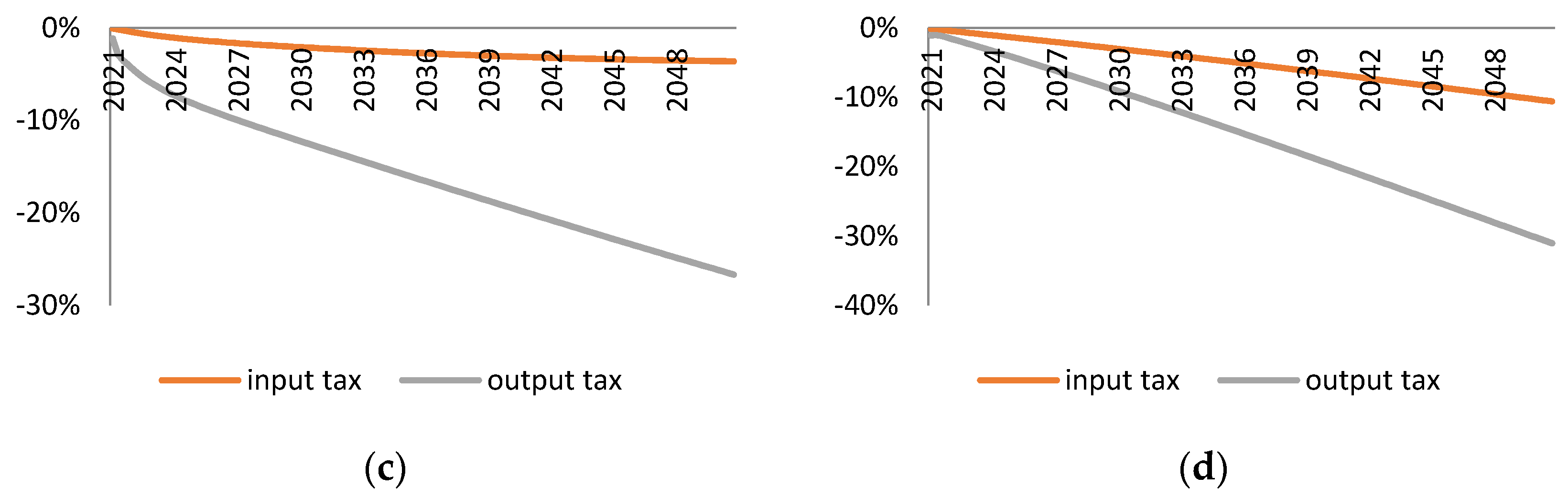
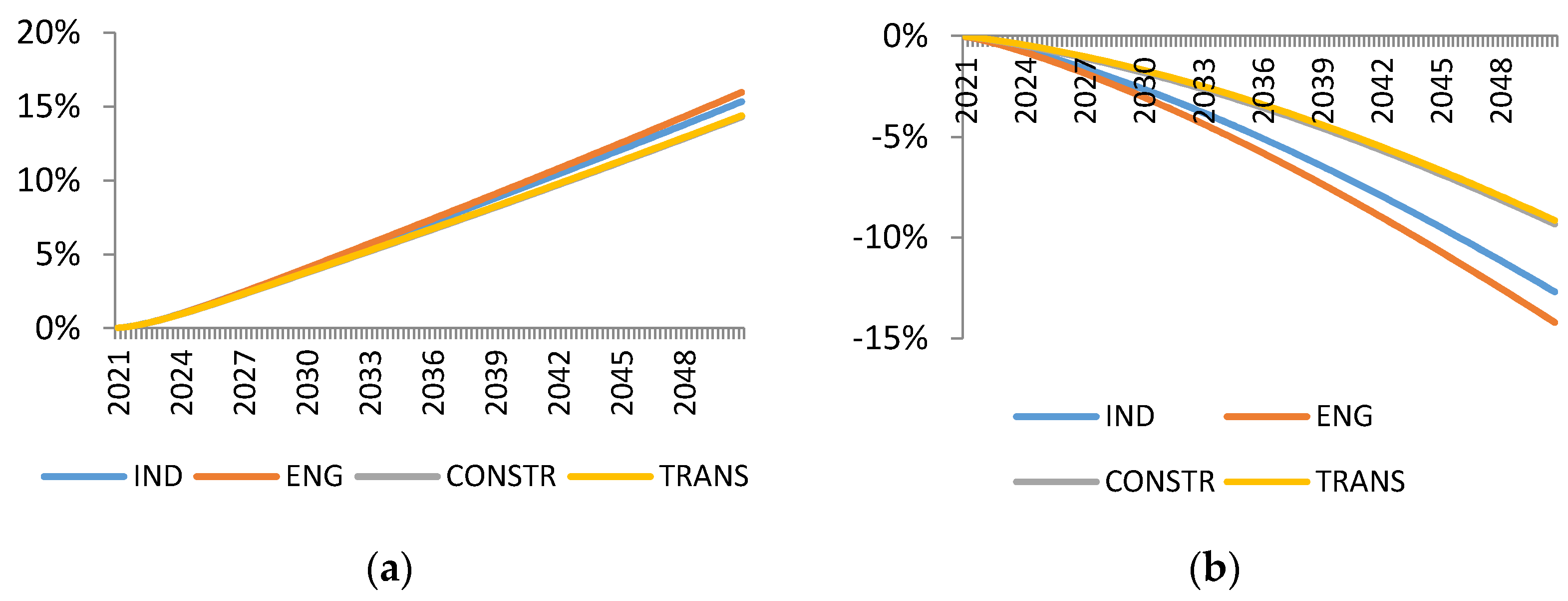
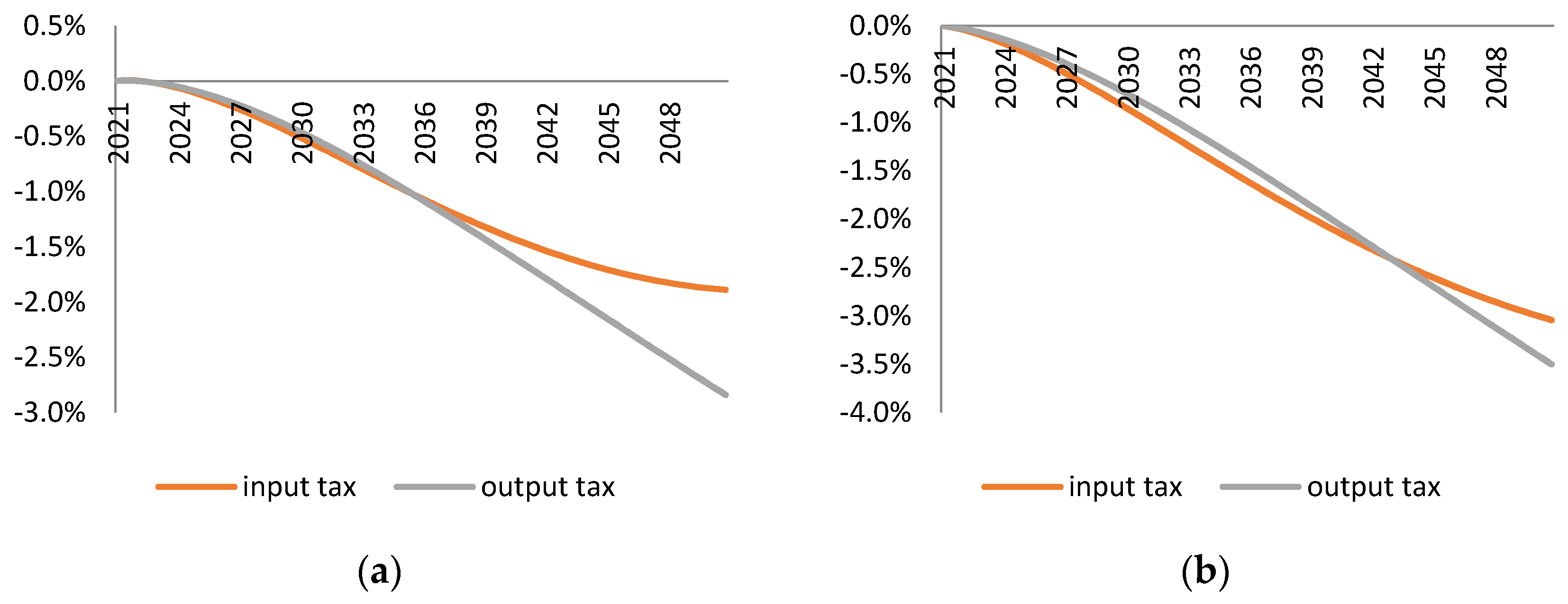
Our simulation results clearly indicate that the reduction of material use through the taxation of material input brings smaller economic costs than the same reduction achieved through the taxation of output in material-intensive sectors. In 2050, the input tax levied on the EU27 from 2021 results in a decline in GDP and employment which is lower by 16 and 17 percentage points respectively in comparison to the effects of the output tax levied in the same period. Furthermore, the input tax achieves the same material reduction target with smaller and less rapid changes in the sector structure of economy. Smaller structural change implies less need for re-skilling of the workforce and, therefore, could potentially entail lower social costs of environmental policy.
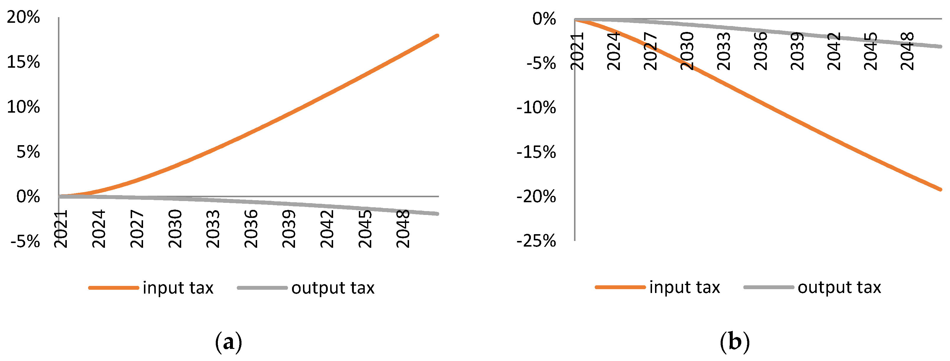
We find that a significant part of the difference between the macroeconomic effects of input and output tax could be traced down to the difference in technological adjustments induced by these taxes. Input tax incentivises firms in material-intensive sectors to invest in material-saving technologies. Since firms substitute materials with technology, they do not need a large cut in production in order to meet the material use reduction target. Indeed, the sensitivity analysis in Section 3.4 shows that when firms do not have an option to invest in material-saving technology, the economic costs of input tax are much larger.
In contrast, the output tax creates no incentives for firms in material intensive industries to substitute materials with technology. A reduction in demand for firms’ products is a direct effect of the output tax. Firms respond to it with a reduction in the use of all factors of production. Since material-saving technology could be viewed as one of the factors, firms will also look for cuts in this domain. Indeed, Figure 13 suggest that the output tax leads to a reduction in material-efficiency. The sensitivity analysis in Section 3.4 indicates that when the firm does not have a possibility to economise on the quality of technology, the reduction in material efficiency is smaller.
In addition to the material reduction approach, we have considered two alternative simulation setups. First, instead of targeting a given reduction in material use, we set a fiscal goal: we identified and simulated the output and input tax rate paths which result in the same budget revenue in 2050. We also found that in this fiscal approach, the input tax involves smaller economic costs (in terms of GDP and employment) than the output tax.
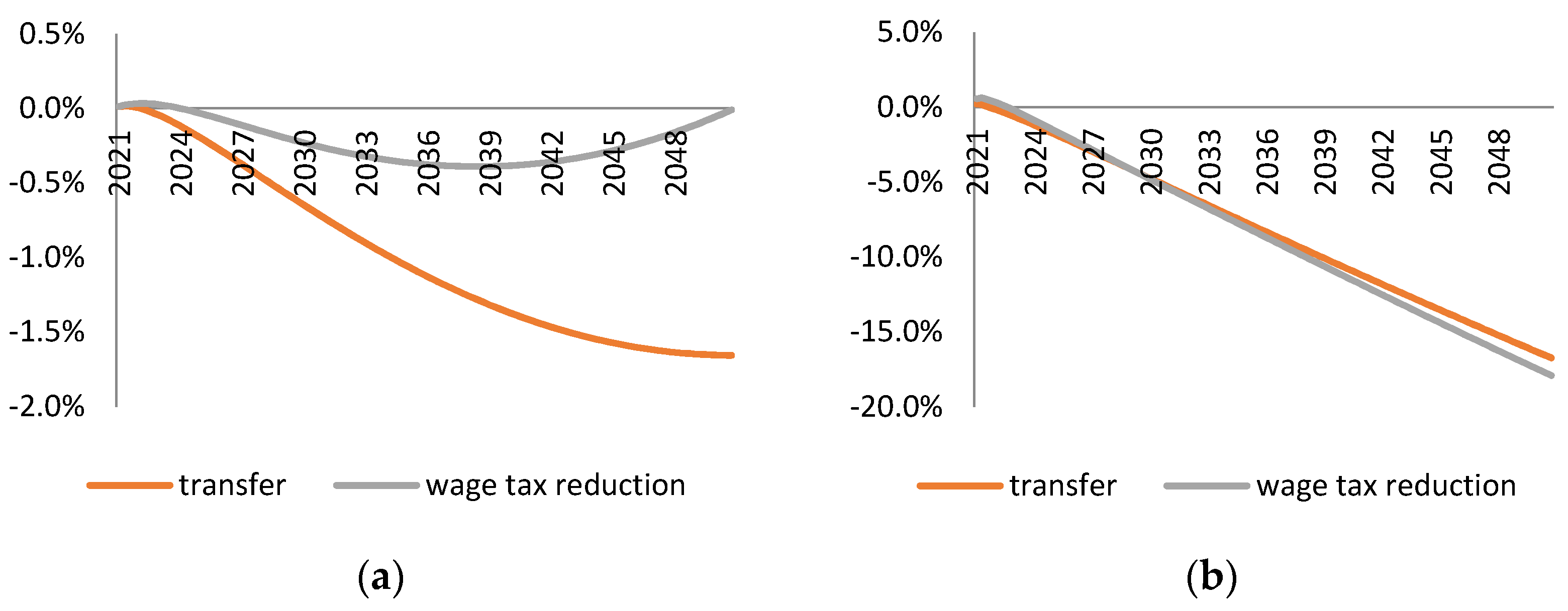
We also considered a scenario in which the tax revenue is partially used to reduce labour taxation. According to the double dividend hypothesis, this shall reduce the negative economic effects of environmental taxes. Indeed, the hypothesis is supported in the case of the input tax. If the tax revenue is used on reduction of the labour tax rate, the input tax has a negligible effect on GDP and employment in the long-run. In contrast, similar recycling of the output tax revenue barely affects the trajectory of GDP and employment loss implied by the output tax with a lump-sum transfer fiscal closure. The reason for this is that the labour tax reduction leads to more production and higher resource use. Thus, the output tax rate has to be even higher to meet the material reduction target which, in turn, introduces even more distortion in the economy.
All in all, we find that the input tax is a better tool to achieve resource decoupling than the output tax. However, output tax is superior in one regard—guaranteeing budgetary revenue. Since the input tax leads to much higher resource efficiency than the output tax, it cuts down its own base to a higher extent than the output tax. Thus, if policy-makers would treat these environmental taxes not only as an instrument to achieve resource decoupling, but also as an additional source of budgetary revenue, they would find the output tax more attractive than suggested by its poorer macroeconomic and resource-efficiency characteristics.

Acknowledgments

The paper has received funding from the European Union’s Seventh Framework Programme under grant agreement No. 308674.

Author Contributions

Marek Antosiewicz developed the DSGE model, contributed to the simulation design and conducted the simulations. Piotr Lewandowski proposed the general methodology, contributed to simulation design and analysis of results. Jan Witajewski-Baltvilks contributed to the simulation design and analysis and discussion of results.

Conflicts of Interest

The authors declare no conflict of interest.

Abbreviations

The following abbreviations are used in this manuscript:
DSGE
Dynamic Stochastic General Equilibrium
IO
Input-Output
EU27
European Union member states except Croatia
GDP
Gross Domestic Product
R&D
Research and Development
CES
Constant Elasticity of Substitution
CPA
Classification of Products by Activity
VAT
Value Added Tax
AGR
Agriculture
RMP
Raw Material Production
IND
Industry
ENG
Energy
CONSTR
Construction
TRANS
Transport
SERV
Market Services
PBL
Public Services

Appendix A

Table A1. Summary of main variables and parameters of firms’ production process.
SymbolInterpretationEquation No.
Variables
Π t s Profit of firm1
K E t s Capital-energy composite good2,3
K t s Stock of capital 2
E N G t s Energy input 2
K L E t s Capital-labour-energy composite good3,4
N t s Labour input 3
Y t s Final good 4
M t s Material input 4,5
M t s , u Material input from sector u 5,6,7
M O t s Material input of all sectors except RMP 5,6
M t , H s , u Domestically-produced material input 7
M t , F s , u Imported material input7
E F F t s Material efficiency5,8
I t s Investment in capital stock 8,9
Z t s Choice of technology level 8,9
I C t s Overall cost of investment 9
Parameters
β Discount factor 1
θ E s Share of energy in K E good2
θ K E s Share of K E in K L E good3
θ M s Share of materials in final good Y 4
θ R M P s Share of raw materials in material good M 5
θ u s Share of sector u material input6
θ H s , u Share of domestic material input in sector u 7
ϵ E s Firm’s short run elasticity of substitution between capital and energy 2
ϵ K E s Firm’s short run elasticity of substitution between K E good and labour3
ϵ M s Firm’s short run elasticity of substitution between K L E good and material input4
ϵ R M P s Firm’s short run elasticity of substitution between raw material input and remaining material input5
ϵ H s Elasticity of substitution between domestic and imported material input7
δ Depreciation rate of capital8
α Degree of technology rigidity which sets medium and long term elasticity of substitution9
1 In the above, t is used to denote time period, s and u are used to index sectors of model.

References

  1. European Commission. Manifesto for a Resource-Efficient Europe; European Commission: Brussels, Belgian, 2012; Available online: http://europa.eu/rapid/press-release_MEMO-12-989_en.htm (accessed on 15 January 2016).
  2. United States Environmental Protection Agency. Beyond RCRA: Prospects for Waste and Materials Management in the Year 2020; United States Environmental Protection Agency: Washington, DC, USA, 2012. Available online: http://www3.epa.gov/epawaste/conserve/smm/vision.htm (accessed on 15 January 2016).
  3. Su, B.; Heshmati, A.; Geng, Y.; Yu, X. A review of the circular economy in China: Moving from rhetoric to implementation. J. Clean. Prod. 2013, 42, 215–227. [Google Scholar] [CrossRef]
  4. Eckermann, F.; Golde, M.; Herczeg, M.; Mazzanti, M.; Montini, A.; Zoboli, R. Resource Taxation and Resource Efficiency along the Value Chain of Mineral Resources; European Environmental Agency: Copenhagen, Denmark, 2012. [Google Scholar]
  5. Popp, D. The effect of new technology on energy consumption. Resour. Energy Econ. 2001, 23, 215–239. [Google Scholar] [CrossRef]
  6. Sue Wing, I. Explaining the declining energy intensity of the U.S. economy. Resour. Energy Econ. 2008, 30, 21–49. [Google Scholar] [CrossRef]
  7. Fæhn, T.; Gómez-Plana, A.G.; Kverndokk, S. Can a carbon permit system reduce Spanish unemployment? Energy Econ. 2009, 31, 595–604. [Google Scholar] [CrossRef]
  8. Popp, D. R&D subsidies and climate policy: Is there a “free lunch”? Clim. Chang. 2006, 77, 311–341. [Google Scholar]
  9. Fischer, C.; Newell, R. Environmental and technology policies for climate mitigation. J. Environ. Econ. Manag. 2008, 55, 142–162. [Google Scholar] [CrossRef]
  10. Gerlagh, R.; van der Zwaan, R. Optionsand instruments for a deep cut in CO2 emissions: Carbon dioxide capture or renewables, taxes or subsidies? Energy J. 2006, 27, 25–48. [Google Scholar] [CrossRef]
  11. Söderholm, P.; Tilton, J.E. Material efficiency: An economic perspective. Resour. Conserv. Recycl. 2012, 61, 75–82. [Google Scholar] [CrossRef]
  12. Allwood, J.M.; Ashby, M.F.; Gutowski, T.G.; Worrell, E. Material efficiency: providing material services with less material production. Philos. Trans. Ser. A 2013. [Google Scholar] [CrossRef] [PubMed]
  13. Skelton, A.C.H.; Allwood, J.M. The incentives for supply chain collaboration to improve material efficiency in the use of steel: An analysis using input output techniques. Ecol. Econ. 2013, 89, 33–42. [Google Scholar] [CrossRef]
  14. Bovenberg, A.; Goulder, L. Optimal environmental taxation in the presence of other taxes: General equilibrium analyses. Am. Econ. Rev. 1996, 86, 985–1000. [Google Scholar]
  15. Goulder, L. Climate change policy’s interactions with the tax system. Energy Econ. 2013, 40, S3–S11. [Google Scholar] [CrossRef]
  16. Linn, J. Energy prices and the adoption of energy-saving technology. Econ. J. 2008, 118, 1986–2012. [Google Scholar] [CrossRef]
  17. Takeda, S. The double dividend from carbon regulations in Japan. J. Jpn. Int. Econ. 2007, 21, 336–364. [Google Scholar] [CrossRef]
  18. Antosiewicz, M.; Kowal, P. Memo III—A Large Scale Multi-Sector DSGE Model; IBS: Warszawa, Poland, 2016. [Google Scholar]
  19. Mortensen, D.T. Equilibrium unemployment dynamics. Int. Econ. Rev. 1999, 40, 889–914. [Google Scholar] [CrossRef]
  20. Pissarides, C.A. Equilibrium Unemployment Theory; MIT Press: Cambridge, MA, USA; London, UK, 2000. [Google Scholar]
  21. Okagawa, A.; Ban, K. Estimation of substitution elasticities for CGE models. In Discussion Papers in Economics and Business; Osaka School of International Public Policy (OSIPP), Osaka University: Osaka, Japan, 2008. [Google Scholar]
  22. Kuper, G.H.; Van Soest, D.P. Path-dependency and input substitution: Implications for energy policy modelling. Energy Econ. 2003, 25, 397–407. [Google Scholar] [CrossRef]
  23. Smets, F.; Wouters, R. An estimated dynamic stochastic general equilibrium model of the euro area. J. Eur. Econ. Assoc. 2003, 1, 1123–1175. [Google Scholar] [CrossRef]
  24. Kemfert, C. Estimated substitution elasticities of a nested CES production function approach for Germany. Energy Econ. 1998, 20, 249–264. [Google Scholar] [CrossRef]
  25. Bucher, R. Mitigation, Adaptation, Technological Change and International Trade: Economic Aspects of Unilateral Climate Policies. Ph.D. Thesis, Universität Bern, Bern, Switzerland, 2011. [Google Scholar]
  26. Koschel, H. Substitution elasticities between capital, labour, material, electricity and fossil fuels in German producing and service sectors. In ZEW Discussion Papers No. 00-31; Center for European Economic Research (ZEW): Mannheim, Germany, 2000. [Google Scholar]
  27. Hooper, P.; Johnson, K.; Marquez, J.R. Trade elasticities for the G-7 countries. In Princeton Studies in International Economics No. 87; Princeton University: Princeton, NJ, USA, 2000. [Google Scholar]
  28. Heathcote, J.; Perri, F. Financial autarky and international business cycles. J. Monet. Econ. 2002, 49, 601–627. [Google Scholar] [CrossRef]
Figure 1. Scheme of model structure.
Sustainability 08 00352 g001
Figure 2. Basic macroeconomic impact of the input and output taxes on gross domestic product, employment, investment, and imports. Results are shown as percent deviations from the baseline scenario; (a) GDP; (b) Employment; (c) Investment; and (d) Imports.
Sustainability 08 00352 g002aSustainability 08 00352 g002b
Figure 3. Tax rates (a) and tax revenue (b) which result in a 20% decrease in the output of the RMP sector. The tax revenue is presented as a percentage of the baseline GDP and does not take into account the endogenous drop in GDP.
Sustainability 08 00352 g003
Figure 4. Effect on material efficiency in selected sectors of the (a) input tax and (b) output tax.
Sustainability 08 00352 g004
Figure 5. Effect on the structure of GDP shown in percentage points with respect to the baseline. (a) GDP structure in 2030; and (b) GDP structure in 2050.
Sustainability 08 00352 g005
Figure 6. Effect on the structure of employment shown in percentage points with respect to the baseline. (a) Employment structure in 2030; and (b) employment structure in 2050.
Sustainability 08 00352 g006
Figure 7. The tax rates and the resulting revenue from the tax (as a share of GDP) — set to approximately achieve 1% of GDP revenue in 2050. (a) tax rates; (b) revenue from tax.
Sustainability 08 00352 g007
Figure 8. Impact on GDP and employment of environmental taxes when rates are set to equate tax revenue. (a) GDP; (b) employment.
Sustainability 08 00352 g008
Figure 9. Effect of environmental taxes on material efficiency in the Industry sector and on material use. (a) Material efficiency in IND; (b) Material use.
Sustainability 08 00352 g009
Figure 10. Effect on GDP under the assumption of 20% revenue recycling to reduce labour tax or transfer closure. (a) input tax; (b) output tax.
Sustainability 08 00352 g010
Figure 11. Effect on employment under the assumption of 20% revenue recycling to reduce labour tax or transfer closure. (a) input tax; (b) output tax.
Sustainability 08 00352 g011
Figure 12. Sensitivity analysis for the effect on GDP with respect to parameter α for the input tax and the output tax. Baseline value used in simulations is 1.5. (a) Sensitivity for the input tax; and (b) sensitivity for the output tax.
Sustainability 08 00352 g012
Figure 13. Sensitivity analysis for effect on material efficiency of Industry sector with respect to parameter α for the input tax and the output tax. Baseline value used in simulations is 1.5. (a) Sensitivity for the input tax; and (b) sensitivity for the output tax.
Sustainability 08 00352 g013
Table 1. Sector structure of model.
Sector NameSector Abbrev.Eurostat CPA Sectors 1
1AgricultureAGRA01, A03, C10-C12
2Raw Material ProductionRMPA02, B
3IndustryINDC except C10-C12
4EnergyENGD, E
5ConstructionCONSTRF
6TransportTRANSH
7Market ServicesSERVG, I, J, K, L, M, N
8Public ServicesPBLO, P, Q, R, S, T, U
1 Letter codes without numbers refer to all subsectors which begin with a given letter.
Table 2. Comparison of final tax rates (for 2050) for transfer and wage tax recycling scenario.
TransferWage Tax Reduction
input tax46.7%51.9%
output tax25.0%44.9%

