1. Introduction
Over the last few decades, a number of energy simulation tools have been developed, such as DOE-2, EnergyPlus, eQuest, ESP-r, IES-VE, TRNSYS,
etc. These tools have been validated by exact analytical solution, inter-program comparison, and a series of experiments with dedicated small test cells [
1,
2,
3,
4,
5,
6,
7,
8,
9]. However, in these studies, exact analytical solution and inter-program comparison were based on idealized assumptions and approximations of buildings, which are in reality very complex, and thus do not guarantee that the tools are fully capable of simulating the complex reality of buildings (e.g., stochastic characteristics of occupant behavior). In addition, empirical validation studies have only been conducted for simple situations under well-controlled and monitored environments. Such experimental conditions differ considerably from the reality, in which buildings are used by stochastic occupants under time-varying uncertain factors (e.g., internal heat gain, infiltration, outdoor intake, weather,
etc.).
Many attempts have been made to use whole building simulation tools for the energy-efficient operation and management of existing buildings [
10,
11]. However, when these tools are applied to existing buildings, the mismatch between the predicted energy use and actual measured energy use [
12], typically termed the performance gap, is an increasing concern [
13,
14,
15,
16]. The magnitude of this performance gap is non-negligible and the measured energy use can be as much as 2.5 times the predicted energy use [
16]. This gap is thus too significant to be overlooked.
Consequently, rather than reporting on a case study in which existing buildings are successfully simulated, this paper discusses several crucial and unresolved issues that contribute to the aforementioned performance gap. The aim of this study is therefore to investigate the issues that need to be solved for energy simulation of an existing building. The issues reported in this paper are derived from an experimental study on an actual office building. The issues to be discussed in this paper are as follows: (1) grey data not ready for simulation; (2) subjective assumptions and judgments on energy modeling; (3) stochastic characteristics of building performance and occupants behavior; (4) verification of model fidelity-comparison of aggregated energy; (5) verification of model fidelity-calibration by trial and error; and (6) use of simulation model for real-time energy management. In addition, this study explains the factors that need to be considered in the process of energy simulation for an actual case study.
2. Target Building
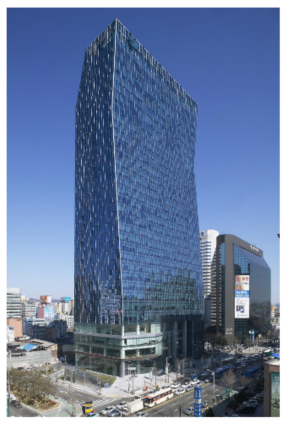
The target building (
Figure 1) is located in Seoul, Korea. The building, constructed in December 2004, is 33 stories above ground and has six underground levels with a total floor area of 91,898 m
2. The primary use of the building is office space, but the lower floors of the building (from the 4th floor underground to the 4th floor above ground) offer several restaurants, multipurpose halls, an auditorium, sports facilities, and conference rooms. The façade of the building is a glass curtain wall system, which has a window-wall ratio of approximately 70%. The glazing is low-e double pane.
The heating, ventilation, and air conditioning (HVAC) system of the building includes the following: Constant Air Volume (CAV) for the lobby, Variable Air Volume (VAV) for offices, Fan Power Unit (FPU) and Fan Coil Unit (FCU) for extreme control spaces requiring constant temperature and humidity, three steam boilers, two absorption chillers and one centrifugal chiller for cooling, two centrifugal chillers for ice storage, and seven heat exchangers. In total, the HVAC plant includes the following: 47 Air Handling Units (AHU), 122 FCU, four packaged air conditioners, five chillers, one ice storage system, five cooling towers, and three boilers.
EnergyPlus was selected as the Building Energy Performance Simulation (BEPS) tool. EnergyPlus is based on the popular features and capabilities of BLAST and DOE-2, including variable time-steps, integrated heat-and-mass balance-based zone simulations, input and output data structures tailored to facilitate a third party module, and numerous HVAC-related functions [
18].
However, the EnergyPlus reference manual [
19] states that EnergyPlus is not intended as a completely flexible tool for direct modeling of the full complexity and exact layout of an actual system. When using EnergyPlus, the simulationist needs to simplify the reality to respond to the capabilities of EnergyPlus. For example, two interconnected hot and chilled water loops that operate at different temperatures and serve different types of equipment cannot be modeled because EnergyPlus does not have a corresponding object to represent [
20]. In another example, EnergyPlus is not able to model multiple HVAC components that serve a single zone since in EnergyPlus, a zone can only be served by one HVAC component [
20].
Maile
et al. [
20] reported on the critical approximations, assumptions, and simplifications of simulation inputs (such as those for infiltration, internal heat gain from people, lights and equipment, wind direction and speed, and data of HVAC components) as well as the shortcomings of BEPS tools. Kim and Park [
21] reported the limitations and issues of EnergyPlus for simulation of the dynamic behavior of a double skin façade. Their study shows significant simulation errors in the prediction of inner/outer glazing temperatures and cavity air temperature caused by the lack of data on convective heat transfer coefficients and wind pressure coefficient [
21].
The following sections describe the issues that need to be solved for a simulation model of the case study office building (
Figure 1). The following sections describe the development process of the simulation model in terms of modeling, calibration, and the use of the simulation model in energy management.
3. Issues in Modeling Process (Issues #1–3)
3.1. Grey Data Not Ready for Simulation (Issue #1)
It was difficult to gather accurate information on simulation inputs of the existing building. Although EnergyPlus provides a default value and several options for uncertain inputs, in-depth knowledge and engineering judgment is still required. Some of the inputs cannot be determined as single deterministic values but should be treated as stochastic values. In such a case, the simulationist should make an aleatory decision. For example, it is difficult to make a robust decision on the determination of respective values for “fraction radiant/convective” with regard to heat gain from people, lights, and equipment.
Similarly, information on architectural/mechanical/electrical systems is insufficient. A simulationist might request relevant information from the engineers and/or designers of each domain. However, the information received is unlikely to be well-structured. When such information is not available, the simulationist should rely on his or her own assumptions.
In the target building, the facility manager was confident about the development of the simulation model, but he was not fully aware of the types of Information and Data (IAD) required and how the IAD were to be used in energy simulation. Thus, the IAD provided by the manager were not well-documented and were not up-to-date. During site visits, it was observed that the use and configuration of several rooms and floors had been changed and several FCUs had been added after construction. Such changes were not recorded, and the authors therefore needed to rely on the manager’s oral description. This issue demonstrates that in most cases, significant effort and time should be spent on acquiring the maintenance history of existing buildings.
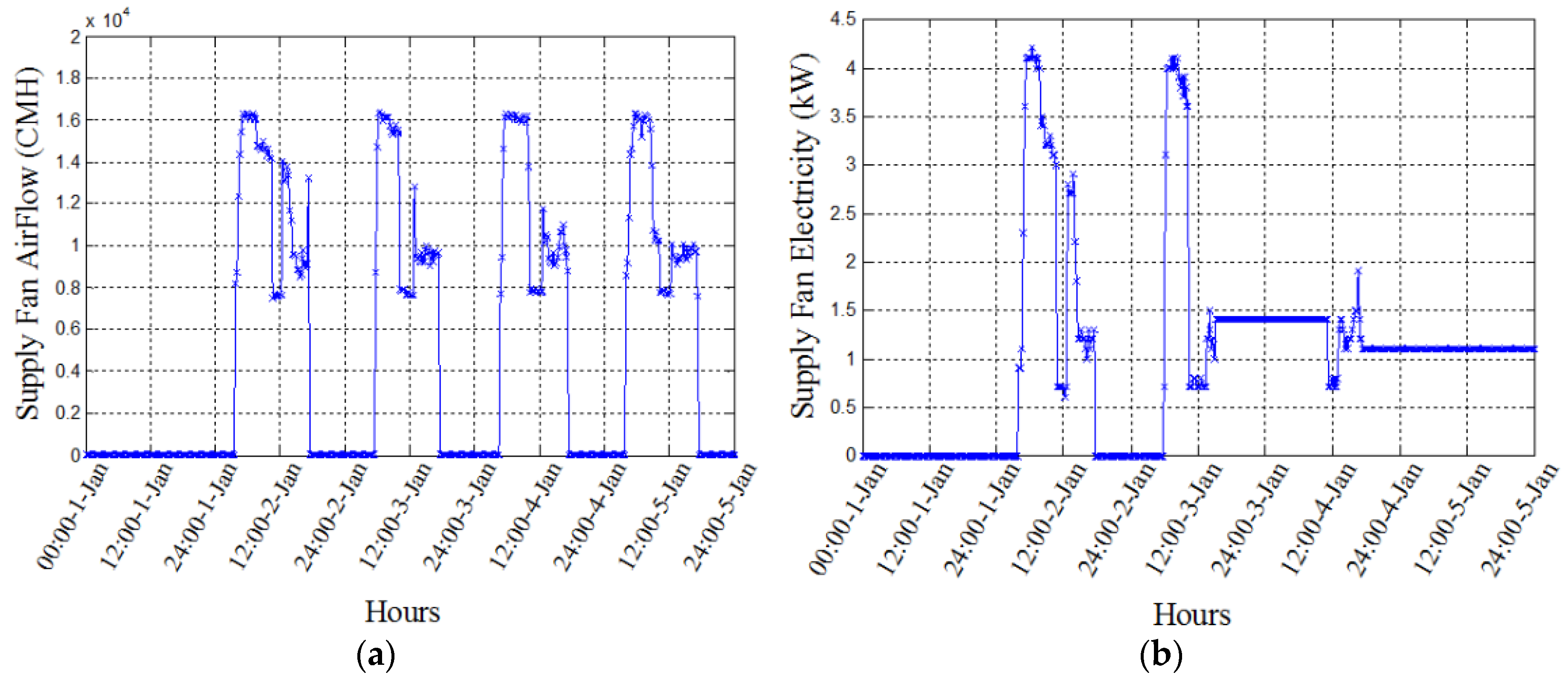
In the target building, the IAD for the fan airflow did not coincide with the IAD for the fan energy use. A Building Energy Management System (BEMS) had been installed and 1692 measurement points were continuously monitored at a sampling time of 15 min.
Figure 2 shows the measured airflow and fan electricity use for the supply fan from January 1 to January 5.
Figure 2a,b is contradictory since the fan airflow rate in
Figure 2a does not match the fan electricity use in
Figure 2b. Thus, we made an assumption that the fan flow was correct based on the building’s usage schedule and the facility manager’s opinion.
3.2. Subjective Assumptions and Judgement on Energy Modeling (Issue #2)
It is usually assumed that the depth of a perimeter zone ranges from 3.5 m to 5.0 m [
19].
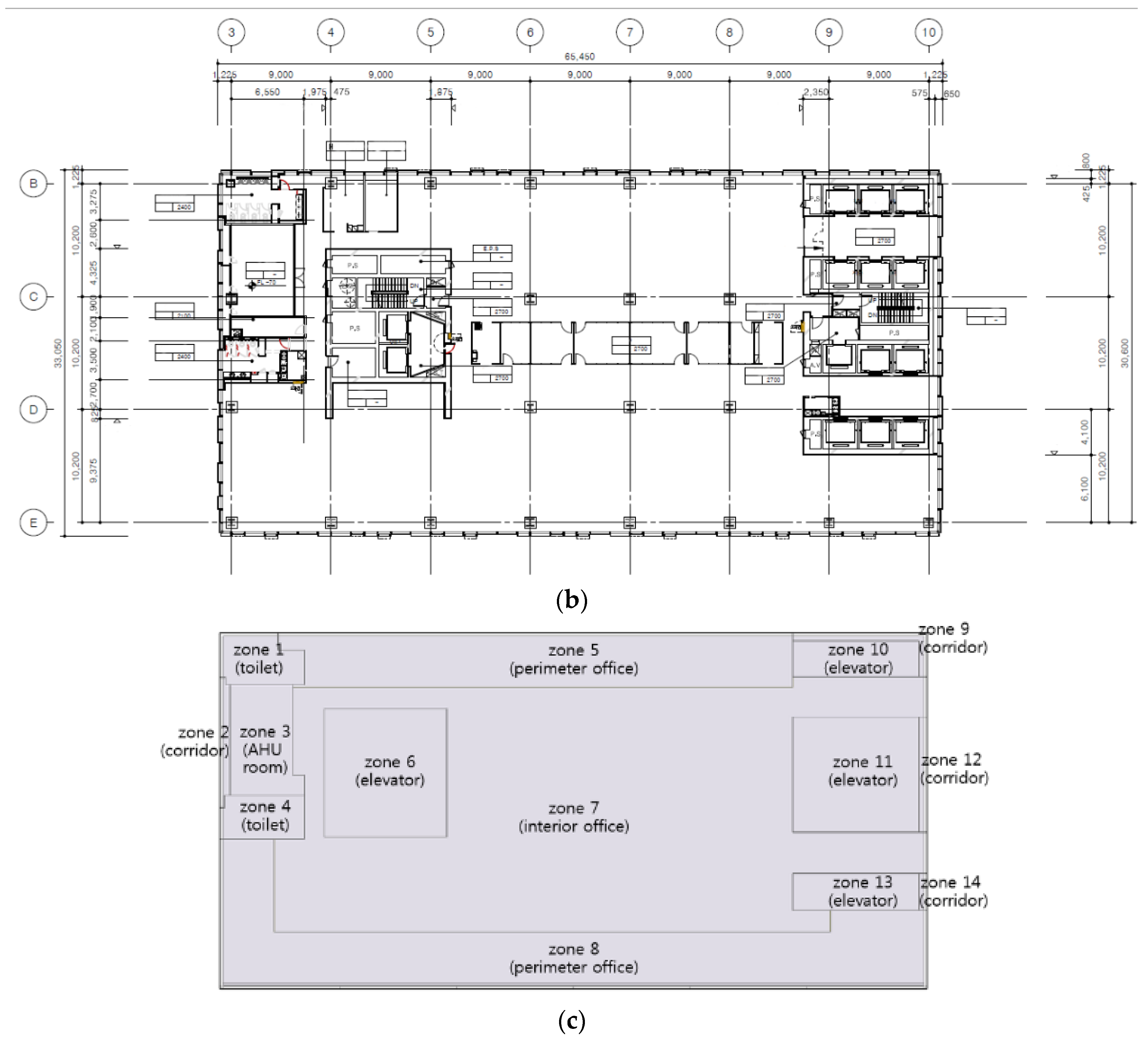
Figure 3 shows the geometry model of the building and the thermal zones of the 7th floor. A typical floor, 7F, has 14 zones including one interior (zone 7), two perimeters (zones 5, 8), two toilets (zones 1, 4), one AHU room (zone 3), four elevator shafts (zones 6, 10, 11, 13), and four corridors (zones 2, 9, 12, 14) (
Figure 3c). Due to the lack of available data, subjective assumptions and judgment are necessary for determining the depth of the perimeter zone (
Figure 3).
EnergyPlus provides information on a number of HVAC systems and controls. Since the Input Output Reference of EnergyPlus is over 2000 pages [
19], it is difficult to acquire an in-depth understanding of all objects and controls. Therefore, a simulationist usually repeatedly uses his or her frequent-use objects.
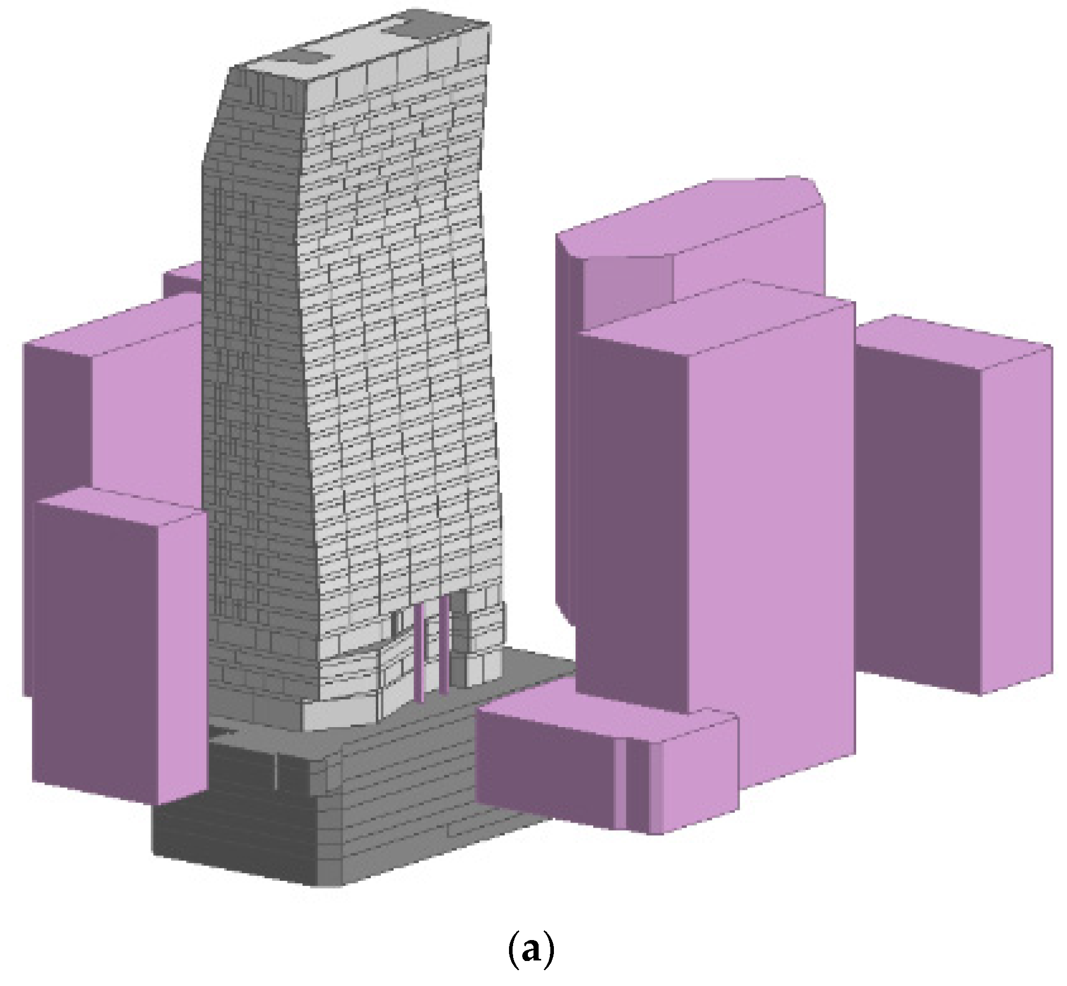
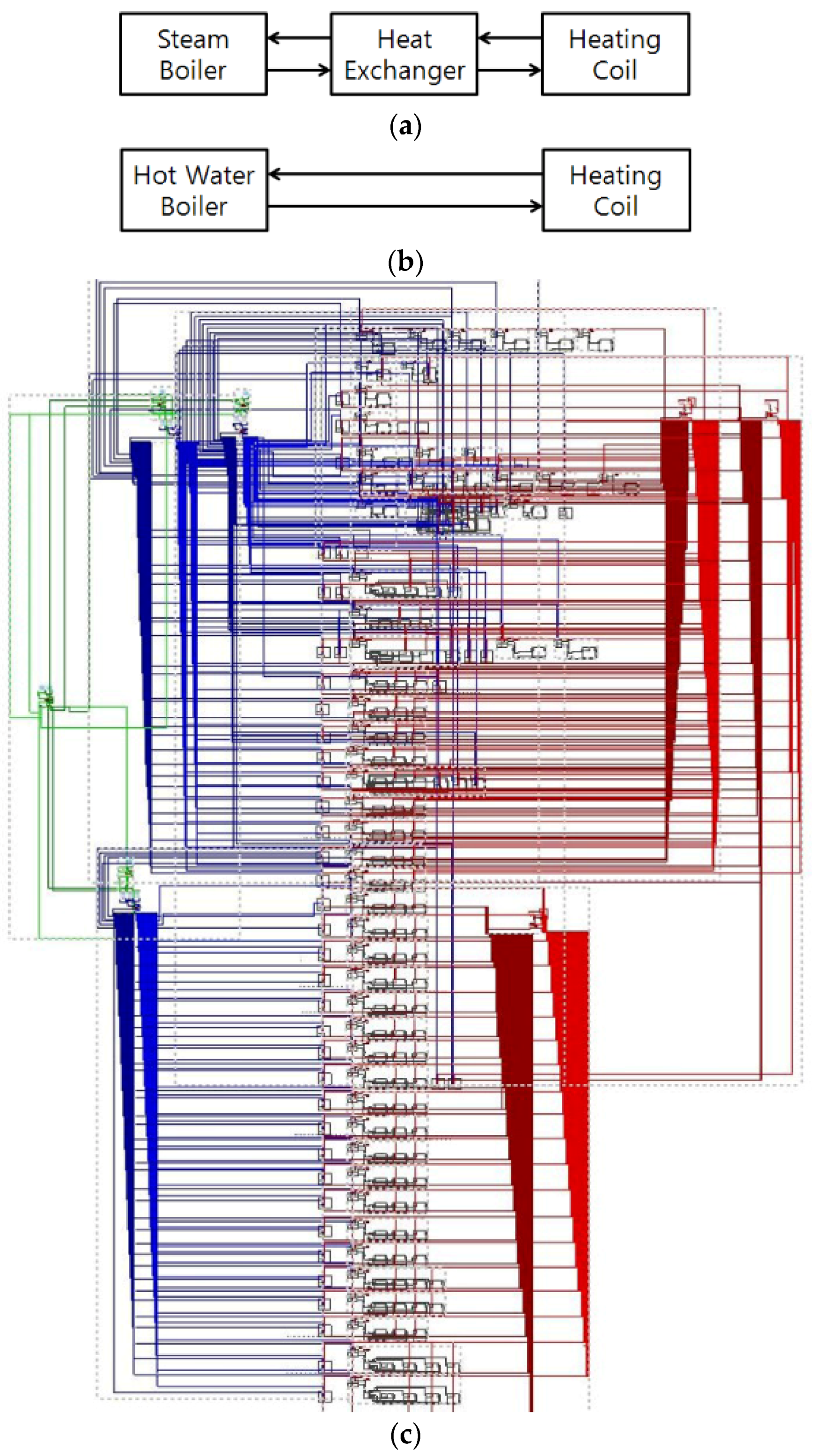
In addition, due to the topology rules, it is not easy to develop a simulation model that is identical to the real building. For example, the target building uses heat exchangers for delivering steam boiler heat to the heating coil (
Figure 4a). Because EnergyPlus does not provide a library for heat exchangers [
19], the heat exchanger was modeled as shown in
Figure 4b. The steam boilers were modeled as hot water boilers, the efficiency of which is the same as that of the steam boilers.
Three plant loops in the building distribute cold water: for floors 6F–34F, for floors B6F–5F, and for special IT rooms. The three loops are connected to the ice storage system for which the three chillers provide cold water. Such interconnection between the three loops, the ice storage system, and the three chillers cannot be modeled due to the topology rules. Hence, each loop was modeled as a stand-alone case. In other words, in the model, each chiller is connected to the ice storage and then to each plant loop (
Figure 4c).
3.3. Stochastic Characteristics of Building Performance and Occupant Behavior (Issue #3)
A detailed energy audit and survey is important to reduce the uncertainty in building energy simulation. However, there are inherent uncertainties due to the stochastic nature of inputs. Internal loads (people, lights, and equipment), indoor set-point temperatures, the operation schedule of plants, and outdoor airflow intake are stochastic inputs and are not easily quantifiable. After several interviews with the manager, the authors realized that, even though advanced automatic controls (e.g., enthalpy control, night-purge control) had been installed, the building was discretionally operated by the facility management team. For example, the outdoor intake rate was frequently changed when occupants complained about stuffy or pungent air. Such irregular operation history has not been documented.
Since an actual building is influenced by stochastic environmental conditions and occupants’ behavior is also stochastic, a deterministic approach is not desirable. As an alternative, uncertainty analysis has previously been introduced [
22,
23,
24].
The deterministic approach, taken by most engineers, is that each input is given as a single value, and a definitive result is derived, whereas the probabilistic approach presents stochastic results based on the stochastic range of inputs. This stochastic approach is considered more objective, rational, and reliable than the deterministic approach since it is based on the stochastic nature of a building and its occupants’ behavior. However, for conducting stochastic simulation, detailed information is needed on inputs (mean, maximum, and minimum values of each input), which include aleatory and epistemic uncertainty. It is worth noting here that epistemic uncertainty literally means a lack of knowledge and information. In other words, it is not easy to take epistemic uncertainty into account.
In addition, the computation time required for uncertainty analysis hinders its application to existing buildings.
Table 1 shows the computation time required for monthly simulation. Since uncertainty, as well as sensitivity analyses, demand at least hundreds of simulation runs, it was not appropriate to investigate the stochastic characteristics of the building.
4. Issues in Calibration Process (Issues #4–5)
4.1. Verification of Model Fidelity-Comparison of Aggregated Energy (Issue #4)
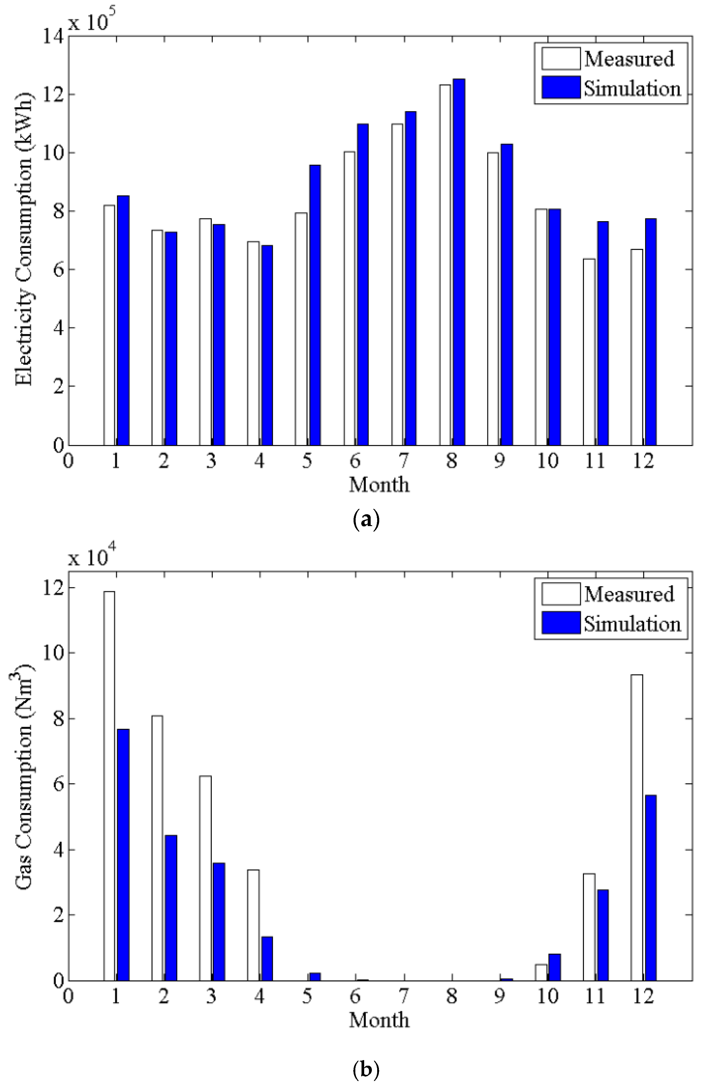
Before attempting to calibrate the model, a comparison was made between the measured monthly energy use and the simulation results (
Table 2,
Figure 5). The simulated electricity consumption (
Figure 5a) has a similar pattern to the actual measured data, and the Mean Bias Error (MBE) and Coefficient of Variation of the Root Mean Squared Error (CVRMSE) are 4.0% and 7.6%, respectively. In contrast to the simulated electricity consumption, the MBE and CVRMSE of gas consumption (
Figure 5b) are −38.4% and 46.5%, respectively, indicating a significant difference between simulated and measured data.
Even though there is good agreement between simulated and measured electricity consumption, this does not guarantee the accuracy of the simulation model with regard to electricity use. Because there was no sub-metered electricity data for fans, chillers, pumps, lights, equipment, etc., the simulated electricity consumption was compared to the aggregated measured electricity data. For better verification of the model fidelity, the simulation prediction must be compared with the sub-metered data (hourly, daily, weekly, etc.). However, in most buildings, sub-metered data is not collected.
4.2. Verification of Model Fidelity-Calibration by Trial and Error (Issue #5)
In general, calibration can be performed in three ways: (1) trial and error; (2) gradient-based optimization to find a set of unknown inputs that minimize the difference between the measurement and prediction; and (3) Bayesian calibration which accounts for the stochastic nature of uncertain inputs. The trial and error method was used in this study due to the relatively low computation time, as mentioned in
Section 3.3.
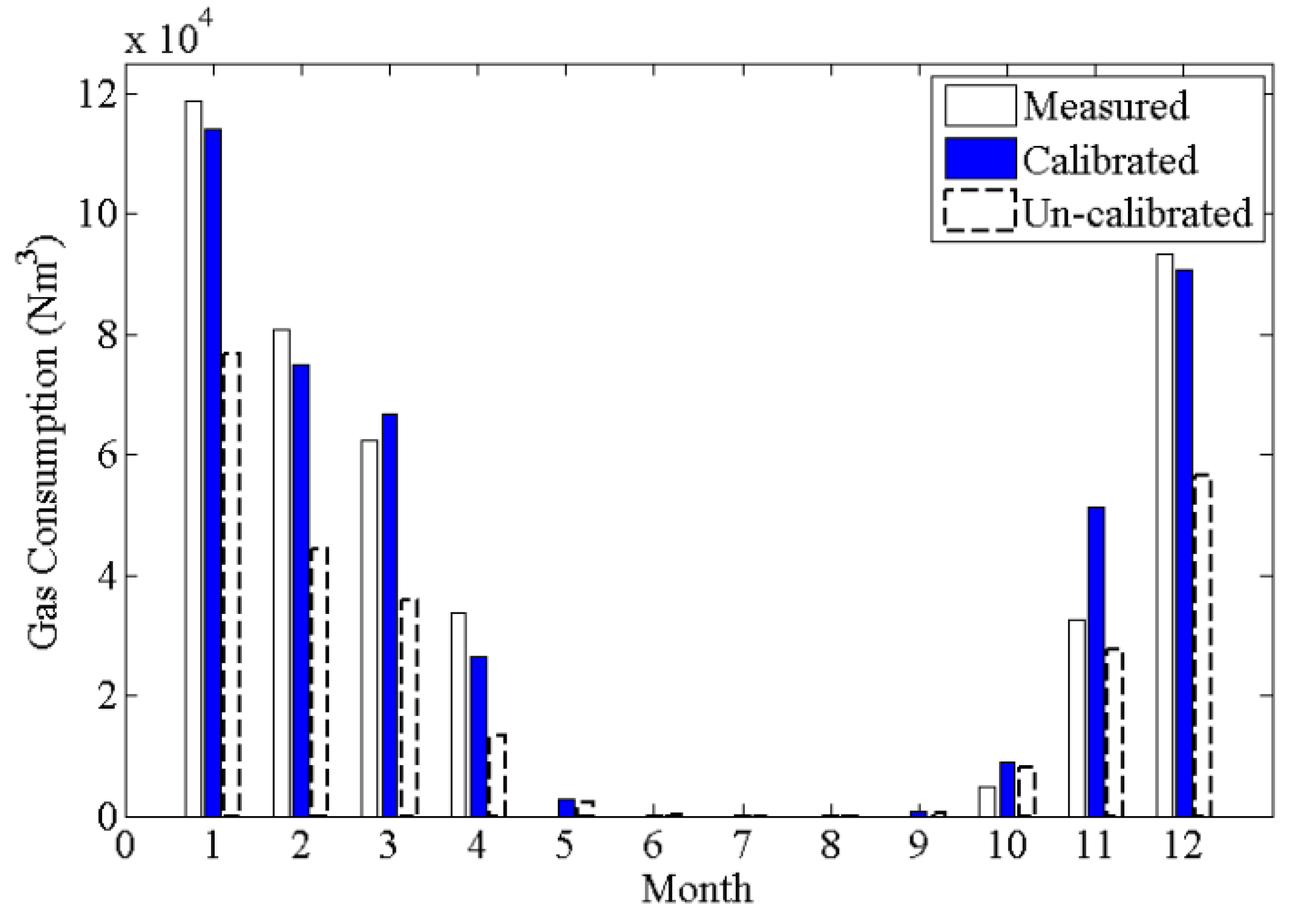
In order to reduce the previously mentioned performance gap in gas prediction (
Table 2,
Figure 5), the BEMS data was checked to estimate the outdoor air intake and the indoor set-point temperature for January (
Table 3). It was found that the initial values for these two inputs differed from the reality. Initially, the boiler efficiency was assumed to be 0.8 due to lack of information. Therefore, in the revised energy model, a boiler efficiency curve from the EnergyPlus data set was applied [
19].
Table 4 and
Figure 6 show a comparison between the measured and calibrated gas consumption. It shows an MBE of 1.5% and a CVRMSE of 14.0% for monthly measurement, which are in good agreement with ASHRAE [
25].
In the “trial and error” calibration approach, only a small set of inputs were tested. Thus, this approach is dependent on subjective intuition and assumptions by engineers. Even though more rigorous calibration methods are available (e.g., optimization function, Bayesian calibration), they were not adopted in this case since they require a considerably greater number of simulation inputs and involve an extensive computation time. In this study, the following simulation inputs remained unidentified:
The chiller’s performance curve: deteriorated thermal characteristics of building envelope (U-values, Solar Heat Gain Coefficient (SHGC)).
Stochastic inputs: HVAC operation, heat and schedule of lighting, schedule of people and equipment.
5. Use of Simulation Model for Real-Time Energy Management (Issue #6)
Most building energy simulation models that are developed in the design stage for the purpose of energy and sustainability ratings are not utilized for the energy management and operation of existing buildings. If the energy simulation model is used for real-time energy management, it can facilitate more rational decision-making by the facility manager. In many building control applications, the simulation model is only used to respond to “what-if” scenarios. A simulation model can be ideally used as part of optimal control which numerically finds the optimal control variables that minimize a given objective function [
26].
In addition, the simulation model should be continuously modified and calibrated during the entire building life cycle. Up-to-date building information (system, internal heat gains, operation schedule, controls, etc.) should be systematically stored and managed in BEMS and should be readily available when required.
6. Conclusions
The purpose of this study was to investigate the issues involved in the energy simulation of an existing building. The authors addressed the following issues: (1) grey data not ready for simulation; (2) subjective assumptions and judgment on energy modeling; (3) stochastic characteristics of building and occupants; (4) stochastic characteristics of building performance and occupants behavior; (4) verification of model fidelity-comparison of aggregated energy; (5) verification of model fidelity-calibration by trial and error; and (6) use of simulation model for real-time energy management. Even though this study was conducted on the single target building, the issues addressed in the paper are scalable to the application of whole building simulation tools to existing buildings.
The selected building is an office building of 33 stories above ground and has 6 underground levels. When developing the simulation model of the building, it was difficult to obtain the relevant data required. The building design and operation data (e.g., drawings, specifications, BEMS data, and operation records) were neither well maintained nor up-to-date (Issue #1). In addition, subjective assumptions and simplifications of the reality had been applied in an ad-hoc fashion (Issue #2). In particular, several cases could not be modeled by the simulation tool due to topology rules. In addition, the stochastic characteristics of building performance and occupants’ behavior (e.g., internal heat generation, occupant behavior, HVAC operation) had been treated in a deterministic manner (Issue #3). After completing the initial simulation model of the building, the simulation results were compared to the energy data. The comparison had been made with the aggregated data rather than the sub-metered data (Issue #4). Although the simulation prediction of electricity use was accurate (MBE of 4.0% and CVRMSE of 7.6%), this does not guarantee “model fidelity”, since the comparison was made between the aggregated measurement and the aggregated prediction (Issue #4). Due to the extensive computation time required for uncertainty analysis, rigorous stochastic parameter estimation (e.g., Bayesian calibration), and optimal control studies for real-time energy management could not be attempted (Issues #3, 5, 6).
For better use of the simulation model for existing buildings, the aforementioned issues need to be solved in the near future. A self-organizing machine learning model could be a candidate for the EnergyPlus model with regard to Issues #1–3. With regard to the reduction of computation time for stochastic performance prediction and real-time optimal control studies (Issues #3, 5, 6), a meta-model could be an alternative (e.g., Support Vector Machine, Gaussian Process model). In addition, IEA Annex 66 has been actively working to solve Issue #4.
Acknowledgments
This work was supported by the Energy Efficiency & Resources Core Technology Program of the Korea Institute of Energy Technology Evaluation and Planning (KETEP), granted financial resource from the Ministry of Trade, Industry & Energy, Republic of Korea. (20152020105550)
Author Contributions
Ki Uhn Ahn, Deuk Woo Kim, Young Jin Kim, and Cheol Soo Park conducted the energy simulation of the target building and analyzed the issues presented in this paper.
Conflicts of Interest
The authors declare no conflict of interest.
Abbreviations
The following abbreviations are used in this manuscript:
| BEPS | Building Energy Performance Simulation |
| MBE | Mean Bias Error |
| CVRMSE | Coefficient of Variation of the Root Mean Squared Error |
| CAV | Constant Air Volume |
| VAV | Variable Air Volume |
| FPU | Fan Power Unit |
| FCU | Fan Coil Unit |
| AHU | Air Handling Units |
| IAD | Information and Data |
| BEMS | Building Energy Management Systems |
References
- Judkoff, R.; Neymark, J. International Energy Agency Building Energy Simulation Test (BESTEST) and Diagnostic Method; Technical Report: NREL/TP-472-6231; National Renewable Energy Laboratory: Golden, CO, USA, 1995.
- International Building Performance Simulation Association (IBPSA). Available online: http://www.ibpsa.org/ (accessed on 7 April 2016).
- ASHRAE Standard 140. American Society of Heating, Refrigerating and Air-Conditioning Engineers, Inc., 2007. Available online: http://www.ashrae.org (accessed on 30 March 2016).
- Strachan, P.A.; Kokogiannakis, G.; Macdonald, I.A. History and development of validation with the esp-r simulation program. Build. Environ. 2008, 43, 601–609. [Google Scholar] [CrossRef] [Green Version]
- Manz, H.; Loutzenhiser, P.; Frank, T.; Strachan, P.A.; Bundi, R.; Maxwell, G. Series of experiments for empirical validation of solar gain modeling in building energy simulation codes-experimental setup, test cell characterization, specifications and uncertainty analysis. Build. Environ. 2006, 41, 1784–1797. [Google Scholar] [CrossRef] [Green Version]
- Reddy, T.A.; Maor, I.; Panjapornpon, C. Calibrating detailed building energy simulation programs with measured data-part 1: General methodology (rp-1051). Hvac&R Res. 2007, 13, 221–241. [Google Scholar]
- Reddy, T.A.; Maor, I.; Panjapornpon, C. Calibrating detailed building energy simulation programs with measured data-part ii: Application, to three case study office buildings (rp-1051). Hvac&R Res. 2007, 13, 243–265. [Google Scholar]
- Williamson, T.J. Predicting building performance: The ethics of computer simulation. Build. Res. Inf. 2010, 38, 401–410. [Google Scholar] [CrossRef]
- Shabi, J.; Reich, Y. Developing an analytical model for planning systems verification, validation and testing processes. Adv. Eng. Inform. 2012, 26, 429–438. [Google Scholar] [CrossRef]
- Database for Analyzing Sustainable and High Performance Building. Available online: http://www.go-gba.org/initatives/dash (accessed on 30 January 2016).
- California Commercial End-Use Survey. Available online: http://www.energy.ca.gov/ceus/ (accessed on 30 January 2016).
- De Wilde, P. The gap between predicted and measured energy performance of buildings: A framework for investigation. Automat. Constr. 2014, 41, 40–49. [Google Scholar] [CrossRef]
- Turner, C.; Frankel, M. Energy Performance of LEED for New Construction Buildings; Final Report; U.S. Green Building Council: Washington, DC, USA, 2008. [Google Scholar]
- Carbon Trust. Closing the Gap: Lessons Learned on Realizing the Potential of Low Carbon Building Design; Carbon Trust: London, UK, 2011. [Google Scholar]
- Zero Carbon Hub. A Review of the Modeling Tools and Assumptions: Topic 4, Closing the Gap between Designed and Built Performance; Zero Carbon Hub: London, UK, 2010. [Google Scholar]
- Menezes, A.C.; Cripps, A.; Bouchlaghem, D.; Buswell, R. Predicted vs. Actual energy performance of non-domestic buildings: Using post-occupancy evaluation data to reduce the performance gap. Appl. Energy 2012, 97, 355–364. [Google Scholar] [CrossRef] [Green Version]
- Viracon. Available online: http://www.viracon.com/projects/view/id/409 (accessed on 30 January 2016).
- Zhou, Y.P.; Wu, J.Y.; Wang, R.Z.; Shiochi, S.; Li, Y.M. Simulation and experimental validation of the variable-refrigerant-volume (vrv) air-conditioning system in energyplus. Energy Build. 2008, 40, 1041–1047. [Google Scholar] [CrossRef]
- EnergyPlus. Department of Energy. Available online: https://energyplus.net/documentation (accessed on 7 April 2016).
- Maile, T.; Fischer, M.; Haymaker, J.; Bazjanac, V. Formalizing Approximations, Assumptions, and Simplifications to Document Limitations in Building Energy Performance Simulation; CIFE Working Paper 126; Stanford University: Stanford, CA, USA, 2012. [Google Scholar]
- Kim, D.W.; Park, C.S. Difficulties and limitations in performance simulation of a double skin facade with energyplus. Energy Build. 2011, 43, 3635–3645. [Google Scholar] [CrossRef]
- MacDonald, I.A. Quantifying the Effects of Uncertainty in Building Simulation. Ph.D. Thesis, University of Strathclyde, Scotland, CA, USA, 2002. [Google Scholar]
- De Wit, S.; Augenbroe, G. Analysis of uncertainty in building design evaluations and its implications. Energy Build. 2002, 34, 951–958. [Google Scholar] [CrossRef]
- Hopfe, C.J. Uncertainty and Sensitivity Analysis in Building Performance Simulation for Decision Support and Design Optimization. Ph.D. Thesis, Technische Universiteit Eindhoven, Eindhoven, The Netherlands, 2009. [Google Scholar]
- ASHRAE Guideline 14. American Society of Heating, Refrigerating and Air-Conditioning Engineers, Inc., 2002. Available online: http://www.ashrae.org (accessed on 30 March 2016).
- Rao, S.S. Engineering Optimization: Theory and Practice; Wiley: New York, NY, USA, 1996. [Google Scholar]
© 2016 by the authors; licensee MDPI, Basel, Switzerland. This article is an open access article distributed under the terms and conditions of the Creative Commons by Attribution (CC-BY) license (http://creativecommons.org/licenses/by/4.0/).


