Detection and Projection of Forest Changes by Using the Markov Chain Model and Cellular Automata

Abstract

The spatio-temporal analysis of land use changes could provide basic information for managing the protection, conservation and production of forestlands, which promotes a sustainable resource use of temperate ecosystems. In this study we modeled and analyzed the spatial and temporal dynamics of land use of a temperate forests in the region of Pueblo Nuevo, Durango, Mexico. Data from the Landsat images Multispectral Scanner (MSS) 1973, Thematic Mapper (TM) 1990, and Operational Land Imager (OLI) 2014 were used. Supervised classification methods were then applied to generate the land use for these years. To validate the land use classifications on the images, the Kappa coefficient was used. The resulting Kappa coefficients were 91%, 92% and 90% for 1973, 1990 and 2014, respectively. The analysis of the change dynamics was assessed with Markov Chains and Cellular Automata (CA), which are based on probabilistic modeling techniques. The Markov Chains and CA show constant changes in land use. The class most affected by these changes is the pine forest. Changes in the extent of temperate forest of the study area were further projected until 2028, indicating that the area of pine forest could be continuously reduced. The results of this study could provide quantitative information, which represents a base for assessing the sustainability in the management of these temperate forest ecosystems and for taking actions to mitigate their degradation.

1. Introduction

During the last decade, the decrement of forest areas has come to attention because of the great environmental impacts on the local, regional and global scales [1,2,3]. The population increase has resulted in high demand for goods and services; inducing changes on the land uses to meet global demands [4]. The forested areas of the planet cover large surfaces representing big carbon reservoirs. However, their reduction has significantly altered the natural landscape and is one of the factors contributing to the global climate change [5,6,7,8]. The forests of Mexico, which are also vulnerable to climate change [9], represent a carbon store of approximately eight billion tons [10], equivalent to the current global CO₂ emissions. The carbon storage capability of these forests is rapidly being lost due to deforestation and degradation processes [11].

Temperate forests occupy the largest forest cover in Mexico, with about 32 million hectares, equivalent to the 18% of its territory. The highest partnerships diversity between pine and oak of the world occurs in this region [12]. However, each year, on average, 40 thousand hectares of temperate forest are lost. The deforestation alters biogeochemical cycles [13]. The expansion of agricultural lands, the illegal logging and the opening of pasturelands to feed cattle on forest areas has resulted in the fragmentation and degradation of the landscape [14]. The quantification of changes in the landscape is important for the understanding of the spatial and structural dynamics of land use and its associated ecological effects [15]. In this regard, it is important to understand the behavior of the areas occupied by forests and the relationships with the abiotic factors involved in their development, distribution and preservation [16]. To analyze the structure, function and dynamics of land use, it is necessary to link spatial patterns with the landscape to quantify the causes and consequences of its evolution [17].

Remote sensing data represent a source of rapid acquisition of land use information, with field supervision methods of low cost [18]. In this regard, the data from the Landsat satellite provides images since 1972, the year of its first mission. This satellite has a worldwide coverage with a medium spatial resolution [19]. Previous studies using information from remote sensing have been developed multitemporal and change detection techniques to monitor the forest dynamics [20,21,22]. Associated with the development of remote sensing, the techniques of land use classification have been refined through the years. One of the techniques commonly used is the maximum likelihood [23,24]. Other method of classification is object-oriented which takes groups of pixels as a unit of analysis. These pixels represent real objects on the ground instead of pixels isolated. The method of neural networks incorporates a multi-information model (spectral response, elevations, thematic maps) related to the statistical distribution of the data [25,26]. In relation to the above, each method offers some reliability in the classification of land use. The best method of classification depends on the interest of the user to discriminate specific categories [27].

Once a classification technique is applied, the comparison and analysis of satellite images from different dates is performed. The difference among the evaluated dates is assessed by map algebra [28,29,30]. Other techniques are based on multivariate analysis through regression of images [31]. The latter method is recently one of the most widely used to predict land use through the variation of this model [32]. However, the logistic regression models cannot quantify the change and serve to perform the temporal analysis [33]. In this regard, the use of Markov chains (MC) and cellular automata (CA), integrated to the spatio-temporal analysis represent an alternative to overcome these limitations. Markov chains and CA are stochastic models that incorporate the interaction effects of the spatial and temporal dynamics [34,35,36]. The Markov prediction methods can serve to analyze the dynamic behavior of land use in a time-space pattern to provide forecasts of future changes that can help in making decisions [37,38]. Some researchers who have applied traditional Markov models have shown their capabilities to describe the trends in the amount of change in land use [38,39,40,41]. Even though the Markov analysis itself can not simulate and predict changes in land use, the combined techniques between MC and CA offer the ability to analyze the spatiotemporal dynamics and also simulate future scenarios. However, Cellular Automata require factors in defining the simulation model of land use [39,40,41].

In this study, we analyzed and modeled the temporal dynamics of land use of a region of temperate forests in the town of Pueblo Nuevo, Durango, Mexico. The traditional Markov model and cellular automata techniques were used to forecast future changes of land use in the study area.

2. Materials and Methods

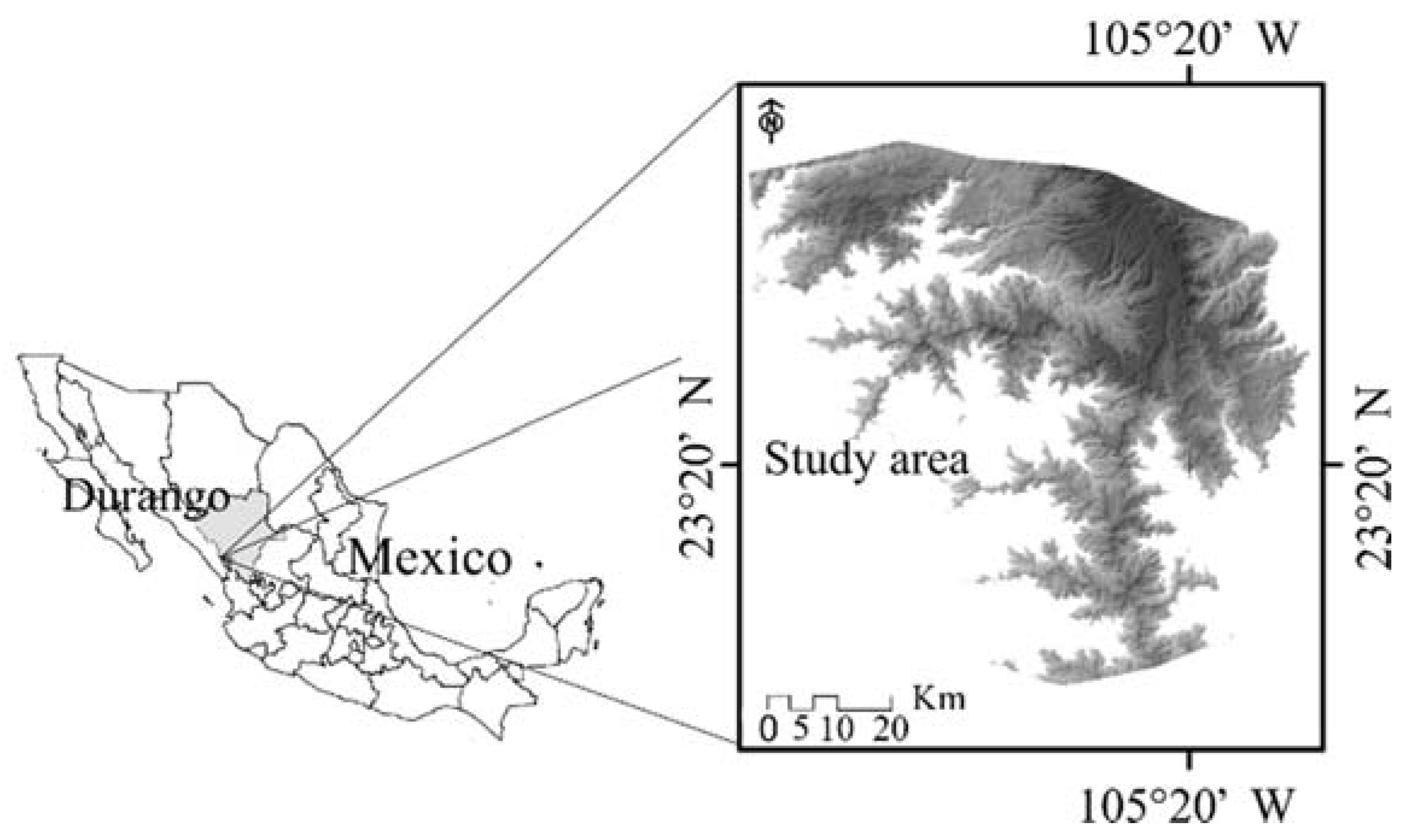
2.1. Study Area

The study area is located in the southern region of the State of Durango, in the municipality of Pueblo Nuevo, with a surface area of 138,710 ha (Figure 1). The vegetation of this region corresponds to a temperate forest. The most abundant forest species are: Quercus sideroxyla Humb. and Bonpl., Q. durifolia V. Seem, Pinus cooperi Ornelasi, P. engelmannii Carr., P. durangensis Schl., P. leiophylla Schl. and Cham., P. teocote Schlech and Cham., and Hardwood species such as Arbutus madrensis and A. tesselata. The herbaceous community is represented by: Bouteloua spp. and Arcthosthaphilos pungens HBK present in open areas with some disturbance.

The climate of the region is temperate humid with summer rains. The air temperature oscillates in the range of 8–26 °C and the precipitation ranges from 800 to 2000 mm. The most abundant soil types are: Leptosol, luvisol, regosol, umbrisol, cambisol, phaeozem and fluvisol [42]. These conditions favor the growth of pine and oak communities, which are the most dominant in the study area.

2.2. Data Collection

Landsat image data were used; the first one from the sensor Landsat Multispectral Scanner (MSS), capture date: 4 April 1973; the second from the Landsat Thematic Mapper (TM), capture date: 26 March 1990 and the third one from the Landsat 8 (Operational Land Imager, OLI), capture date: 6 May 2014. The information was acquired from the US Geological Survey (USGS). The data from the Landsat MSS has four spectral bands, with a spatial resolution of 60 m; however, it was re-sampled to 30 m. The TM sensor has seven spectral bands and its spatial resolution is 30 m. Data from the Landsat 8 has nine spectral bands with a spatial resolution of 30 m in bands 1–7 and 9, while its eighth band (panchromatic) has a spatial resolution of 15 m. The bands from the evaluated sensors are located in the wavelengths of the optical and infrared regions of the electromagnetic spectrum. To make a coherent superposition of the classified images, the final resolution utilized for all of them was 30 m. This was necessary for later analysis carried out with CA.

2.3. Data Pre-Processing

The satellite images from 1973, 1990 and 2014 were radiometrically corrected. The conversion from digital numbers (DN’s) to reflectance values was performed with the process called top of the atmosphere (TOA). This process is necessary to make comparisons among the images from different dates. The radiometric conversion for the Landsat MSS and TM sensors was performed by following the Equations (1) and (2), where the spectral radiance ($L_{\lambda }$) and the TOA reflectance (${\rho }_{\lambda }$) were obtained:

$$L_{\lambda }=\left(\left(Lma{x}_{\lambda }-Lmi{n}_{\lambda }\right)/\left(QCALmax-QCALmin\right)\right)\times \left(QCAL-QCALmin\right)+Lmi{n}_{\lambda }$$

(1)

$${\rho }_{\lambda }=\frac{\pi \times L_{\lambda }\times d^2}{ESU{N}_{\lambda }\times cos{\theta }_s}$$

(2)

where $QCAL$ is DN, $Lmi{n}_{\lambda }$ is the spectral radiance scales to $QCALmin$, $Lma{x}_{\lambda }$ is the spectral radiance scales to $QCALmax,QCALmin$ is the minimum quantized calibrated pixel value, $QCALmax$ is the máximum quantized calibrated pixel value, $d$ is the distance from the earth to the sun, $ESU{N}_{\lambda }$ is the mean solar exoatmospheric irradiance, and ${\theta }_s$ is the solar zenith angle.

In the case of the data from the Landsat 8, the radiometric conversion was performed by applying the Equation (3).

$${\rho }_{\lambda }^{*}=\frac{{\rho }^{\lambda ´}}{sin{\theta }_{SE}}$$

(3)

where ${\rho }^{\lambda ´}$ is the TOA planetary reflactance, with correction for solar angle, and ${\theta }_{SE}$ is the local sun elevation angle.

For reflectance normalization of the images from 1973 and 1990 the image from Landsat 8 was used. This process allows to making a modification on the histograms by improving the brightness values in the images from 1973 and 1990, taking as a reference the image from 2014. This process allows to minimizing the spectral variations of the land use covers [43].

2.4. Image Classification

For the supervised classification, the method of maximum likelihood was used. This method uses training areas as polygons and decision rules of maximum likelihood (Equation (4)) to classify images. Three classified land use maps derived from the Landsat MSS 1973, the Landsat TM 1990 and the Landsat sensor OLI 2014 were obtained; one from each sensor. The three classified images were adjusted to the same spatial resolution of 30 m. Given that the vegetation of the study area predominantly consisted of natural temperate forests, distributed in a scarp topography, the water harvesting takes place mainly through infiltration and runoff processes towards lower places in the watershed. Then, the accumulation of water or the presence of water bodies in the zone was practically null. Therefore, based on the dominance of forest species and their ecological and economical importance in the region, the land uses classified in all the images were: Open Areas (Oa), Oak forests (Of) and Pine forests (Pf).

$$gi \left(x\right)=In p \left(\omega i\right)-\frac{1}{2} In |{{\displaystyle \sum }}^{\text{}}i|-\frac{1}{2} {\left(x- m_i\right)}^T{{\displaystyle \sum }}^{\text{}}{i}^{-1} \left(x- m_i\right)$$

(4)

where: $g$i = class, x = n-dimensional data (where n is the number of bands), p (${\omega }_i$) = probability that class ${\omega }_i$ appears in the image and that is assumed for all classes, |∑_i| = determinant of co-variance matrix data from class ${\omega }_i$, and ∑_i⁻¹ = inverse matrix, m_i = vector.

2.5. Spectral Separability

The canopy structure of the plants belonging to each land use played an important role during the discrimination process. The canopy reflectance in the infrared range (SWIR) is closely related to the water absorption. Meanwhile, the energy dispersion is also caused by the canopy structure and by the aerial space among the leaves [44,45]. The spectral separability was determined by the Jeffrey-Matusita distance ($JM$) [46], according to Equation (5). This method includes the value of the Bathacharyya distance (Equation (6)) [47].

$$JM=2\left(1-e^{-B}\right)$$

(5)

$$B=\frac{1}{8}{\left(m_1-m_2\right)}^2\frac{2}{{\sigma }_1^2+{\sigma }_1^2}+\frac{1}{2}In\frac{{\sigma }_1^2{\sigma }_1^2}{2{\sigma }_1^2{\sigma }_1^2}$$

(6)

where $B$ is the Bhattacharyya distance, $m_1$, $m_2$ and σ1, σ2 are the class means and variances, respectively. The $JM$ distance has values from 0 to 2. A value of 2 indicates a complete separability between two classes and lower values indicate misclassified classes.

2.6. Classification Accuracy

The Kappa coefficient was used to validate the classifications (Equation 7) by employing 300 control points for each year, taken from the compositions of false color images. The Kappa coefficient and the error matrix are considered as common techniques in measuring the accuracy of thematic maps generated by the classification process [48]. Measurements of particular categories of classification can be verified with field data or reference data [49].

$$K_{APPA}= \frac{N{{{\displaystyle \sum }}^{\text{}}}^K{X}_{ii }{{{\displaystyle \sum }}^{\text{}}}^k\left(X_{i+}\times X_{+i}\right)}{N^2-{{{\displaystyle \sum }}^{\text{}}}^k\left(X_{i+}\times X_{+i}\right)}$$

(7)

where: K_APPA = Kappa index, k = number of matrix files, Xii = observation number on row i and column I (along the diagonal), X_i+ and X_+i = total marginal for row i and column i, respectively, N = total number of observations.

2.7. Land Use and Land Cover Change Using Markov Chain

The simulation technique used to predict the change in land use was the Markov Chains. The Markov Chains is a stochastic process model that describes the probability of change from one state to another, i.e., from one land use type to another, using a transition probability matrix [34,35,36]. The transition probability would be the probability that a land cover type (pixels) at the time t₀ changes to another land cover type in the time t₁. Therefore, changes in land use between the dates were used to develop a probability transition matrix and then predict land uses for a future time. This matrix is the result of the crossing between the images by setting a proportional error. The transition probability maps are elaborated from the three land uses generated through the process of classification and these are used to calculate projections of possible changes between the specified times. The mathematical expression of the transition probability is:

$${\displaystyle \sum }_{I=1}^{m}Pij=1 i=1,2\dots \dots m$$

(8)

$$P=\left(Pij\right)=\begin{array}{ccc}P11& P12\dots & P1m\\ P21& P12& P2m\\ Pm1& Pn2& Pmm\end{array}$$

(9)

where: Pij = the probability of transition from one land use to a another, m = the type of land use of the area studied, Pij values are within the range 0–1.

The combination of Markov and Cellular Automata (CA_Markov) allows simulating the evolution of the geographical area represented by pixels. Each pixel can take a value from a finite set of states. All pixels are affected by a transition function that takes as arguments the measured values and values of the neighboring pixels as a function of time. For the study area, the transition function was determined based on the difference between 1990 and 2014. CA_Markov then used this transition function to predict the land cover for 2028. In other words, the transition probability matrix, created from the changes observed between 1990 and 2014, the transition probability maps of 2014 and each scenario were used to produce maps of land use for the year 2028. In an iterative process CA_Markov uses the transition probability maps of each land cover to establish the inherent suitability of each pixel to change from one land use type to another. To assign a weight of suitability to the pixels that are away from the pixel analyzed, a 5 × 5 filter (Figure 2) was used [50]. Since the probability of changes during the years analyzed stays constant, any year after 2014 can be projected. However, projections in the short term are more realistic than projections in the long term, so we run the simulation until 2028.

2.8. Validation of the Model

The validation of the prediction model of land use change was carried out by using the simulation result of land use from Markov for 2014. This, with the reference map obtained from the supervised classification process of the same year. Through the comparison of the observed and simulated values, the model was validated. A transition matrix was generated to analyze the probability of change in land use.

2.9. Cellular Automata (CA)

Cellular Automata is a simulation model where the space and time are discrete variables and interactions assigned are local variables [51]. Cellular automata analysis was carried out by the module of CA_Markov in the software Idrisi Selva. This module uses the output of the analysis of the Markov Chain and predicts the land use for a future time. To predict the land use, the supervised classifications for the three periods were used.

3. Results and Discussion

3.1. Spectral Serability

Table 1. $JM$ distance for the land uses of Oa vs. Of, Oa vs. Pf and Of vs. Pf.

Landsat MSS	Landsat TM	Landsat OLI8	Band Name	Oa vs. Of	OA vs. Pf	Of vs. Pf
1	1	2	Blue	1.33	1.39	0.88
2	2	3	Green	1.23	1.40	0.97
3	3	4	Red	1.11	1.38	1.13
4	4	5	NIR	1.45	1.46	1.65
	5	6	SWIR1	1.48	1.65	1.67
	7	7	SWIR2	1.47	1.48	1.52

shows the results of the $JM$ distance for the land uses analyzed in this study corresponding to the years 1973, 1990 and 2014. According to the bands processed from the Landsat sensors analyzed, it can be observed that the fifth band of the sensors TM and OLI8 show the highest values of spectral separability for the clases OA vs. Of, OA vs. Pf and Of vs. Pf ($JM$ = 1.48, 1.65, 1.67). The analysis also shows that the infrared band (band 4 in Landsat MSS; band 4 in Landsat TM; band 5 in Landsat OLI8) plays a key role in the discrimination of the land uses studied.

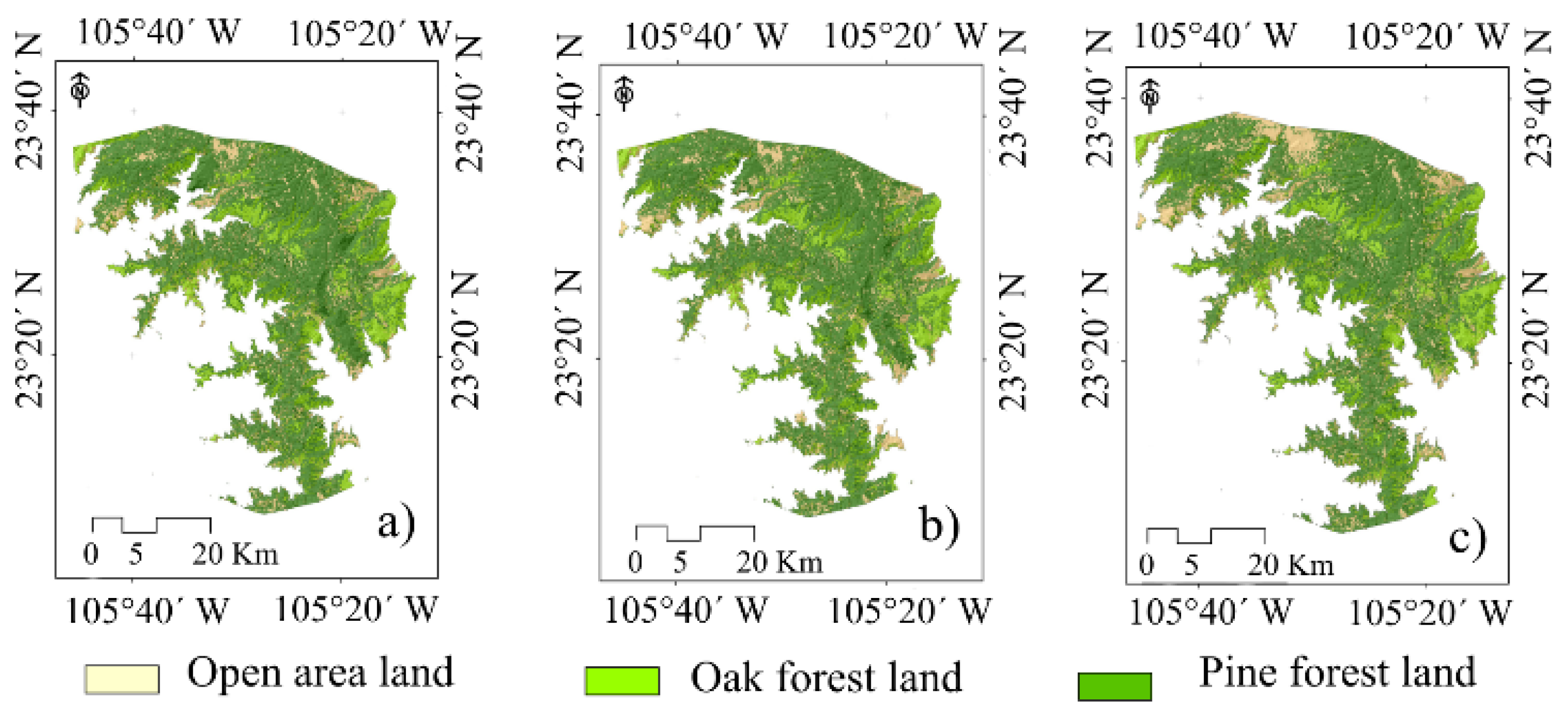
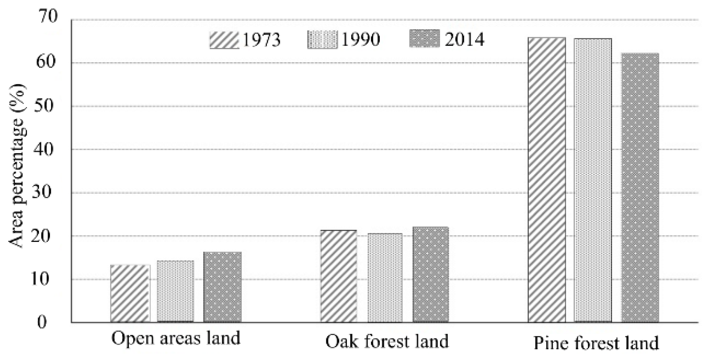
3.2. Land Use Classification 1973, 1990 and 2014

Three types of land use were determined for the study area, as they were the most representative of the region (Figure 3). The land use of OA was the one presenting the least spatial distribution in the study area. Grassland areas, populated areas and scrubland areas represented this class. According to the natural potential of the region, these areas were not significant in terms of their spatial extent, followed by the class Of and the class Pf. The land use classification of 2014 was the one presenting the largest errors. The estimated global precision, based on the error matrix, was 92% with a kappa index of 0.90. In this year, the lowest precision was presented by the class of OA, both for the producer precision (92%) and the user precision (91%). The land use classification for the year 1990 showed the highest precision, showing less errors in the spectral characterization of classes, and registering a global precision of 94% with a kappa index of 0.92. For the year 1973 the global precision was 93% with a kappa index of 0.91 (

Table 2. Accuracy assessment of the classified land use maps.

Years/Classes	Classification Accuracy
	Producer’s Accuracy (%)	User’s Accuracy (%)	Overall Accuracy (%)	Cohen´s Kappa
1973			93	0.91
Open areas	93	91
Oak forest	94	94
Pine forest	93	93
1990			94	0.92
Open areas	93	92
Oak forest	92	91
Pine forest	96	92
2014			92	0.90
Open areas	91	91
Oak forest	93	95
Pine forest	94	94

). The final global precision reached for the maps was due mainly to the individual precision obtained for each of the three classes. All of them presented producer precisions within the range of 91%–96% and user precisions within the range of 91%–95%.

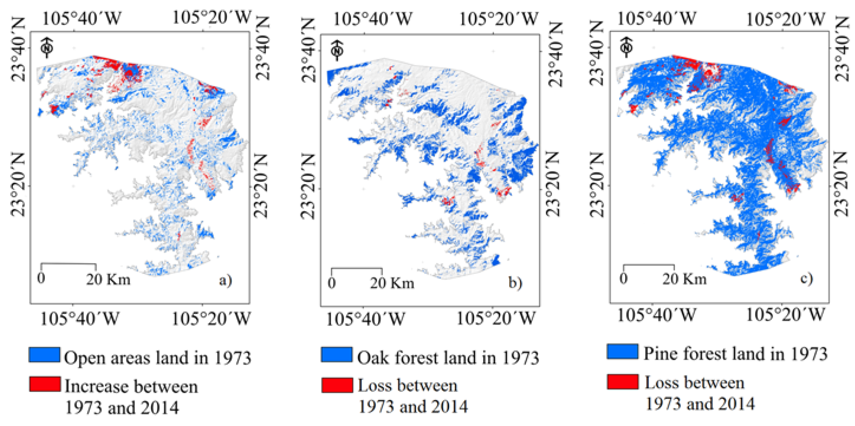
3.3. Land Use and Land Cover Change (1973–2014)

Once the land uses were obtained through the method of supervised classification, we analyzed the land use change dynamics.

Table 3. Areas (ha), percentages and changes of land use for the years 1973, 1990 and 2014.

Land Use	Area (in ha) and Percentages (%)						Changes (in ha)
	1973		1990		2014		1973–1990	1990–2014
	Area	%	Area	%	Area	%
Open areas land	18,304.57	13.20	19,742.13	14.23	22,363.47	16.12	−1437.56	−2621.34
Oak Forest land	29,327.24	21.14	28,418.46	20.49	30,397.13	21.91	908.78	−1978.67
Pine Forest land	91,078.73	65.66	90,549.94	65.28	85,949.94	61.96	528.79	4600

shows the surface change dynamics in each class. From 1973 to 1990 the class of OA increased by 1437 ha, the class of Of lose 908 ha and the class of Pf lose 528 ha. The increase of the class occurred at the expense of the classes of Of and Pf. However, the most important change dynamics occurred during the last 24 years of the period analyzed (1990–2014). The class of Pf showed the biggest loss with 4600 ha. During this period the classes of Of and OA increased by 1928 ha and 2621 ha, respectively (Figure 4).

The temporal land use changes during the period analyzed (1973–2014) are shown in Figure 5. The land use change in the region resulted in a steady loss of Pf, represented by a decrement of 5128.79 ha. In contrast, the classes of OA and Of increased by 4059 ha and 1070 ha, respectively. These changes could be attributed to the wood harvesting that takes place in the region. This activity is perhaps one of the main factors that impact the sustainability of the temperate forests of the region and threatens the communities living in such forest [52,53,54].

3.4. Validation of Land use Change Projection

For the model validation, we compared the simulated land use areas by Markov Chains with the actual ones. The results are shown in

Table 4. Comparison of land use in 2014 generated by supervised classification processes against predicted by Markov techniques and CA.

Land Use	Observed 14		Predictor 14
	Area (ha)	Total Area (%)	Area (ha)	Total Area (%)
Open areas	22,363.44	16	21,988.89	16
Oak forest	30,397.13	22	30,989.21	22
Pine forest	85,949.94	62	85,732.41	62

, in which three land use types presented relative errors lower than 4%. The best agreement was shown by the pine forest type, where the actual area is 85,949.9 ha, while the corresponding simulated area is 85,732.41 ha. Thus, the developed Markov model is verified to effectively predict area change of land use in the future. Meanwhile, the Markov–Cellular Automata’s overall simulation success was 96.12% in 2014. In addition, the kappa coefficient was determined to be 0.92, also showing a high precision. Therefore, the Markov–CA model can be used to forecast the spatial distribution of land use in the future.

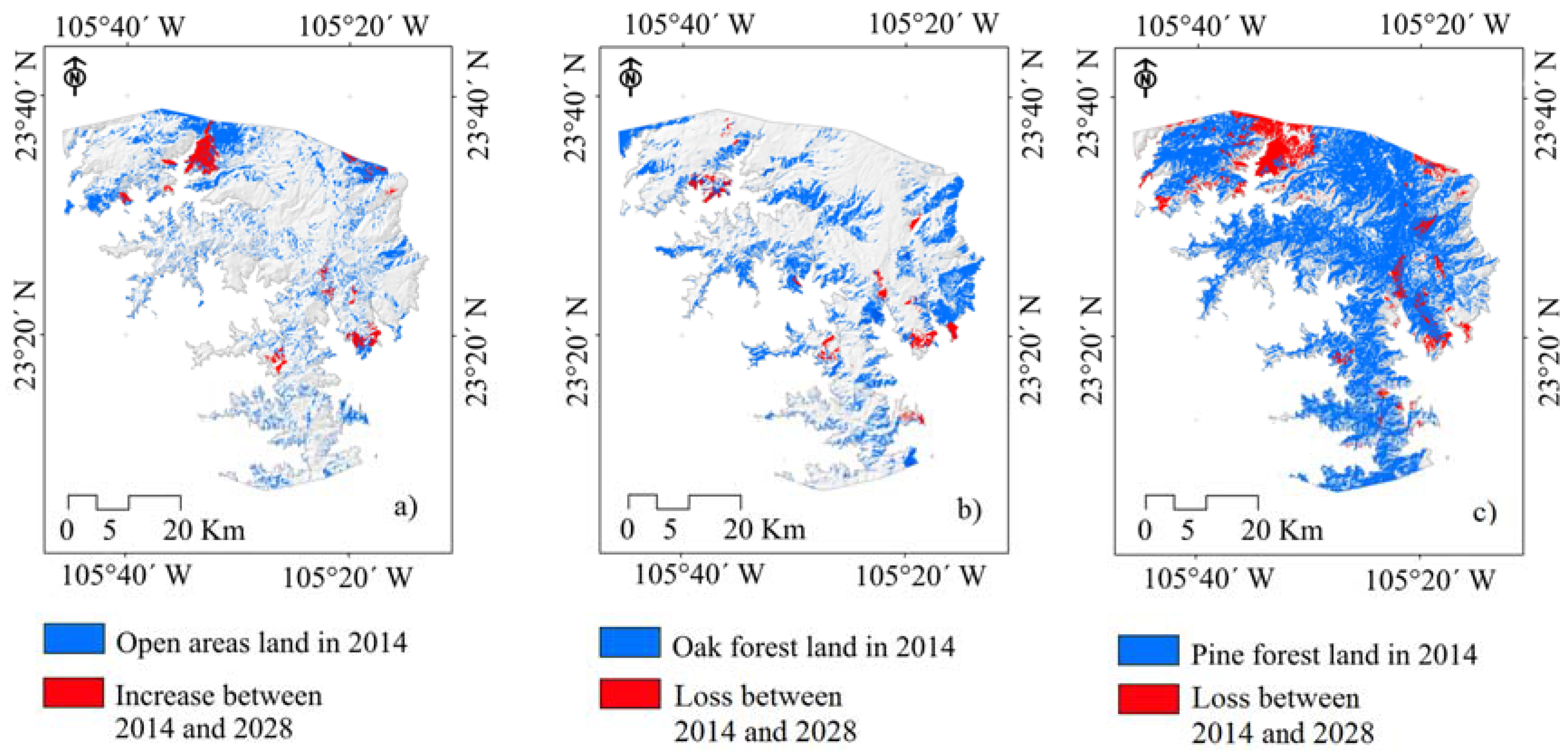
3.5. Land Use Change Projection

The land use was projected using Markov’s transition probability matrices (

Table 5. Transition probability matrices of land use changes for three periods (%).

	Pine Forest	Oak Forest	Open Areas
1973–1990
Pine forest	0.543	0.167	0.289
Oak forest	0.187	0.315	0.498
Open areas	0.276	0.204	0.519
1990–2014
Pine forest	0.422	0.208	0.369
Oak forest	0.308	0.294	0.398
Open areas	0.255	0.289	0.456
2014–2028
Pine forest	0.379	0.229	0.392
Oak forest	0.399	0.246	0.354
Open areas	0.252	0.294	0.453

). A transition matrix summarizes the dynamics of each land use. The results show how the class of OA expanded at the expense of the classes of Pf and Of. The most significant changes occurred during the period 1990–2014, where the class of Pf had the highest loss with 4600 ha. The probability of change in this category was 42%, compared to 54% for the period 1973–1990. In the last period studied, the classes of OA and Of increased its surface area in 2621 and 1978 ha, respectively. The transition matrix showed values from 25% to 30% for this same period, whereas for the period of 1973–1990 the values were 18% and 27%. The loss of Pf area during the evaluated period reveals some level of degradation of these ecosystems, which reduces the environmental sustainability of these forests. The changes were mainly caused by wood harvesting, as well as construction of roads and power lines [55,56,57].

The land use projection for the year 2028 was based on the transition probability matrices. Figure 6 shows the spatial distribution of the land use classes for 2028. According to the transition matrix presented in Table 4, the class of OA will continue to increase its area in 25% while the classes of Pf and Of will decrease their surface in 37% and 39%, respectively. These changes will be induced by the anthropogenic activities that take place in the area. The Global Partnership on Forest Landscape Restoration reports that more than 2000 million hectares of forestland were completely cleared worldwide over the past centuries. These areas are in a state of degradation [58].

4. Conclusions

The simulation of the spatio-temporal dynamics of temperate forests represent an alternative for the mapping of forest ecosystems in a given time series. The classification of satellite images showed a good level of accuracy with respect to ground reference data, as supported for the values of the Kappa coefficient. In the period of 1973–2014 the class of Pf lost more than five thousand hectares. This land was converted to other land uses. The principal causes contributing to this decline were manly forestry, construction of roads and power lines. The analysis of the trends in land use change by using Markov Chains and CA shows the influence of these activities in the region. The land uses of the temperate forests projected for 2028 show a similar trend when compared to the period 1973–2014, where 4800 ha of pines will be probably lost. The open areas will increase to 4200 ha, and the oak forest will increase by 1400 ha. It is important that the government institutions involved with the forest management policies take action in the conservation, protection and production of the temperate forest ecosystems. Overall, the combined methods in this study demonstrate the usefulness in applying remote sensing to monitor spatial and temporal changes of temperate forests. The results of this study could provide quantitative information, which represents a base for assessing the sustainability in the management of these temperate forest ecosystems.

References

1. Cabrera, V.A.; Vilalta, M.J. Patterns of forest decline and regeneration across scots pine populations. Ecosystems 2013, 16, 323–335. [Google Scholar] [CrossRef]
2. Chen, F.C.; Son, T.N.; Chang, B.N.; Chen, R.C.; Chang, Y.L.; Valdez, M.; Centeno, G.; Thompson, A.C.; Aceituno, L.J. Multi-decadal mangrove forest change detection and prediction in Honduras, Central America, with Landsat imagery and a Markov chain model. Remote Sens. 2013, 5, 6408–6426. [Google Scholar] [CrossRef]
3. Lambin, F.E.; Meyfroidt, P. Global land use change, economic globalization, and the looming land scarcity. PNAS 2011, 108, 3465–3472. [Google Scholar] [CrossRef] [PubMed]
4. Yu, X.J.; Ng, C.N. Spatial and temporal dynamics of urban sprawl along two urban-rural transects A case study of Guangzhou, China. Landsc. Urban Plan. 2007, 79, 96–109. [Google Scholar] [CrossRef]
5. Leuzinger, S.; Luo, Y.; Beier, C.; Dieleman, W.; Vicca, S.; Körner, C. Do global change experiments overestimate impacts on terrestrial ecosystems? Trends Ecol. Evol. 2011, 26, 236–241. [Google Scholar] [CrossRef] [PubMed]
6. Watson, R.T.; Noble, I.R.; Bolin, B.; Ravindranath, N.H.; Verardo, D.J.; Dokken, D.J. Land Use, Land-Use Change and Forestry: A Special Report of the Intergovernmental Panel on Climate Change, 1st ed.; Cambridge University Press: Cambridge, UK, 2000; p. 388. [Google Scholar]
7. Abdalla, M.; Saunders, M.; Hastings, A.; Williams, M.; Smith, P.; Osborne, B.; Lanigan, G.; Jones, M.B. Simulating the impacts of land use in Northwest Europe on Net Ecosystem Exchange (NEE): The role of arable ecosystems, grasslands and forest plantations in climate change mitigation. Sci. Total Environ. 2013, 465, 325–336. [Google Scholar] [CrossRef] [PubMed]
8. Dale, V.H. The relationship between land-use change and climate change. Ecol. Appl. 1997, 7, 753–769. [Google Scholar] [CrossRef]
9. Villers, R.L.; Trejo, V. Assessment of the vulnerability of forest ecosystem to climate change in Mexico. Clim. Res. 1997, 9, 87–93. [Google Scholar] [CrossRef]
10. Mansera, O.; Ordóñez, M.J.; Dirzo, R. Carbon emissions from Mexican forests: Current situation and long-term scenarios. Clim. Change 1997, 35, 265–295. [Google Scholar] [CrossRef]
11. Grimm, N.B.; Grove, J.M.; Pickett, S.T.A.; Redman, C.L. Integrated approaches to long-term studies of urban ecological systems. Bioscience 2000, 50, 571–584. [Google Scholar] [CrossRef]
12. González, E.M.S.; González, E.M.; Tena, F.A.; González, R.L.; López, E.L. Vegetación de la sierra madre occidental, México: Una síntesis. Acta Bot. Mex. 2012, 100, 351–403. [Google Scholar]
13. Potter, S.C. Terrestrial biomass and the effects of deforestation on the global carbon cycle results from a model of primary production using satellite observation. Bioscience 1999, 49, 769–778. [Google Scholar] [CrossRef]
14. Manjarrez-Domínguez, C.; Pinedo-Alvarez, A.; Pinedo-Alvarez, C.; Villarreal-Guerrero, F.; Cortes-Palacios, L. Vegetation landscape analysis due to land use changes on arid lands. Pol. J. Ecol. 2015, 63, 272–279. [Google Scholar] [CrossRef]
15. Turner, M. Landscape ecology in North America: Past, present and future. Ecology 2005, 86, 1967–1974. [Google Scholar] [CrossRef]
16. Bormann, F.H.; Likens, G.E. Pattern and Process in a Forested Ecosystem, 1st ed.; Springer-Verlag: New York, NY, USA, 1994; p. 245. [Google Scholar]
17. Kabba, S.T.V.; Li, J. Analysis of land use and land cover changes, and their ecological implications in Wuhan, China. J. Geogr. Geol. 2011, 3, 104–118. [Google Scholar] [CrossRef]
18. Pal, M.; Mather, P.M. Assessment of the effectiveness of support vector machines for hyperspectral data. Future Gener. Comput. Syst. 2004, 20, 1215–1225. [Google Scholar] [CrossRef]
19. Hansen, M.C.; Loveland, T.R. A review of large are monitoring of land cover change using Landsat data. Remote Sens. Environ. 2012, 122, 66–74. [Google Scholar] [CrossRef]
20. Tang, J.; Wang, L.; Zhang, S. Investigating landscape pattern and its dynamics in Daqing, China. Int. J. Remote Sens. 2005, 26, 2259–2280. [Google Scholar] [CrossRef]
21. Read, J.M.; Lam, N.S. Spatial methods for characterizing land cover and detecting land-cover changes for the tropics. Int. J. Remote Sens. 2002, 23, 2457–2474. [Google Scholar] [CrossRef]
22. Coppin, P.; Jonckheere, I.; Nackaerts, K.; Muys, B.; Lambin, E. Digital change detection methods in ecosystem monitoring: A review. Int. J. Remote Sens. 2004, 25, 1565–1596. [Google Scholar] [CrossRef]
23. Bolstad, P.; Lillesand, T.M. Rapid maximum likelihood classification. Photogramm. Eng. Remote Sens. 1991, 57, 67–74. [Google Scholar]
24. Franklin, J.; Woodcock, C.E.; Warbington, R. Multi-attribute vegetation maps of forest services lands in California supporting resource management decisions. Photogramm. Eng. Remote. Sens. 2000, 66, 1209–1217. [Google Scholar]
25. Mas, J.F.; Flores, J.J. The application of artificial neural networks to the analysis of remotely sensed data. Int. J. Remote Sens. 2008, 29, 617–663. [Google Scholar] [CrossRef]
26. Lin, Y.P.; Chu, H.J.; Wu, C.F.; Verburg, P.H. Predictive ability of logistic regression, auto-logistic regression and neural network models in empirical land-use change modeling—A case study. Int. J. Geogr. Inf. Sci. 2011, 25, 65–87. [Google Scholar] [CrossRef] [Green Version]
27. Brown, D.G.; Page, S.; Riolo, R.; Zellner, M.; Rand, W. Path dependence and the validation of agent-based spatial models of land use. Int. J. Geogr. Inf. Sci. 2005, 19, 153–174. [Google Scholar]
28. Dewan, A.M.; Yamaguchi, Y.; Rahman, M.Z. Dynamics of land use/cover changes and the analysis of landscape fragmentation in Dhaka Metropolitan, Bangladesh. GeoJournal 2012, 77, 315–330. [Google Scholar] [CrossRef]
29. Guild, L.; Cohen, W.; Kauffman, J. Detection of deforestation and land conversion in Bondonia, Brazil using change detection techniques. Int. J. Remote Sens. 2004, 25, 731–750. [Google Scholar] [CrossRef]
30. Pinedo, A.C.; Pinedo, A.A.; Martinez, Q.R.M. Analysis of deforested areas in the north central region of the Sierra Madre Occidental, Chihuahua, México. Tecnociencia Chihuahua 2007, 1, 36–43. [Google Scholar]
31. Yuan, D.; Elvidge, C. NALC land cover change detection pilot study: Washington DC data experiments. Remote Sens. Environ. 1998, 66, 166–178. [Google Scholar] [CrossRef]
32. Verhagen, P. Case Studies in Archaeological Predictive Modeling; Amsterdam University Press: Amsterdam, The Netherlands, 2007; p. 224. [Google Scholar]
33. Lambin, E.F. Modelling Deforestation Processes: A Review; Office for Official Publications of the European Community: Brussels, Belgium, 1994. [Google Scholar]
34. Glenn, D.C.; Lewin, R.K.; Peet, T.T.V. Plant Succession: Theory and Prediction; Chapman & Hall: London, UK, 1992. [Google Scholar]
35. Hu, Z.; Lo, C. Modeling urban growth in Atlanta using logistic regression. Comput. Environ. Urban Syst. 2007, 31, 667–688. [Google Scholar] [CrossRef]
36. Cabral, P.; Zamyatin, A. Markov Processes in Modeling Land Use and Land Cover Changes in Sintra-Cascais, Portugal. Dyna 2009, 191–198. [Google Scholar]
37. Liu, Y. Modelling Urban Development with Geographical Information Systems and Cellular Automata; Taylor & Francis Group: New York, NY, USA, 2009; p. 177. [Google Scholar]
38. Lepš, J. Mathematical modelling of ecological succesion–A review. Folia Geobot. Phytotax. 1988, 23, 79–94. [Google Scholar] [CrossRef]
39. Arsanjani, J.J.; Kainz, W.; Mousivand, A.J. Tracking dynamic land-use change using spatially explicit Markov Chain based on cellular automata: The case of Tehran. Int. J. Image Data Fusion 2011, 2, 329–345. [Google Scholar] [CrossRef]
40. Camacho, O.M.T.; Pontius, R.G., Jr.; Paegelow, M.; Mas, J.F. Comparison of simulation models in terms of quantity and allocation of land chance. Environ. Model. Softw. 2015, 69, 214–221. [Google Scholar] [CrossRef]
41. Yang, X.; Zheng, X.-Q.; Lv, L.N. A spatiotemporal model of land use change based on ant colony optimization, Markov chain and cellular automata. Ecol. Model. 2012, 233, 11–19. [Google Scholar] [CrossRef]
42. INEGI (Instituto Nacional de Estadística, Geografía e Informática) 2012—Información Nacional, por Entidad Federativa y Municipios. Available online: www.inegi.org.mx/ (accessed on 24 February 2016). (in Spanish).
43. Richards, J.A.; Jia, X. Remote Sensing Digital Image Analysis: An Introduction, 4th ed.; Springer-Verlag: Berlin, Germany, 2006; p. 439. [Google Scholar]
44. Eastman, J.R.; Van Fossen, M.E.; Solarzano, L.A. Transition Potential Modeling for Land Cover Change. In GIS, Analysis, Spatial, Modeling; Maguire, D.J., Goodchild, M.F., Batty, M., Eds.; ESRI Press: Redlands, CA, USA, 2005; p. 386. [Google Scholar]
45. Mitsova, D.; Shuster, W.; Wang, X. A cellular automata model of land cover change to integrate urban growth with open space conservation. Landsc. Urban Plan. 2011, 99, 141–153. [Google Scholar] [CrossRef]
46. Bhattacharyya, A. On a measure of divergence between two statistical populations defined by their probability distributions. Bull. Calcutta Math. Soc. 1943, 35, 99–109. [Google Scholar]
47. Eastman, R.; Idrisi, T. Guide to GIS and Image Processing, Manual Version 16.02; Clark University: Worcester, MA, USA, 2009; p. 342. [Google Scholar]
48. Smits, P.C.; Dellepiane, S.G.; Schowengerdt, R.A. Quality assessment of image classification algorithms for land-cover mapping: A review and a proposal for a cost-based approach. Int. J. Remote Sens. 1999, 20, 1461–1486. [Google Scholar] [CrossRef]
49. Congalton, R.G.; Oderwald, R.G.; Mead, R.A. Assessing Landsat classification accuracy using discrete multivariate analysis statistical techniques. Photogramm. Eng. Remote Sens. 1983, 49, 1671–1678. [Google Scholar]
50. Mousivand, A.J.; Alimohammadi, S.A.; Shayan, S. A New Approach of Predicting Land Use and Land Cover Changes by Satellite Imagery and Markov chain model (Case study: Tehran). Ph.D. Thesis, Tarbiat Modares University, Tehran, Iran, 2007. [Google Scholar]
51. Benenson, I.; Torrens, P.M. Geosimulation: Automata-Based Modeling of Urban Phenomena; Wiley: Chichester, UK, 2004; pp. 1–287. [Google Scholar]
52. Strigul, N.; Florescu, I.; Welden, R.A.; Michalczewski, F. Modelling of forest stand dynamics using Markov chains. Environ. Model. Softw. 2012, 31, 64–65. [Google Scholar] [CrossRef]
53. Clark Labs. IDRISI Geographic Information Systems and Remote Sensing Software; Clark Labs: Worcester, MA, USA, 2006. [Google Scholar]
54. Wolfram, S. Cellular automata as models of complexity. Nature 1984, 311, 419–424. [Google Scholar] [CrossRef]
55. Vazquez, Q.G.; Pinedo, A.A.; Manjarrez, D.C.; De Leon, M.G.; Hernandez, R.A. Analysis of temperate forest fragmentation using spatial medium-resolution remote sensing in Pueblo Nuevo, Durango. Tecnociencia Chihuahua 2013, 7, 88–98. [Google Scholar]
56. Renteria, A.B.; Treviño, G.E.; Navar, C.J.; Aguirre, C.O.; Silva, C.I. Woody fuel assessment in the ejido Pueblo Nuevo, Durango. Rev. Chapingo 2005, 11, 51–56. [Google Scholar]
57. Pompa, G.M.; Zapata, M.M.; Hernandez, D.C.; Rodriguez, T.E. Geospatial model as strategy to prevent forest fires: A case study. J. Environ. Prot. 2012, 3, 1034–1038. [Google Scholar] [CrossRef]
58. FAO. Food and Agriculture Organization. State of the World’s Forest. Available online: http://www.fao.org/docrep/016/i3010e/i3010e.pdf (accessed on 24 February 2016 2016).
Figure 1. Location of the study area, municipality of Pueblo Nuevo, Durango.
Sustainability 08 00236 g001
Figure 2. 5 × 5 filter configuration used in CA Markov.
Sustainability 08 00236 g002
Figure 3. Land use/land cover maps for the years (a) 1973; (b) 1990 and (c) 2014.
Sustainability 08 00236 g003
Figure 4. Percentage of area occupied by each land use in 1973, 1990 and 2014.
Sustainability 08 00236 g004
Figure 5. Changes in Land uses between 1973 and 2014: (a) Open areas; (b) Oak forest and (c) Pine forest.
Sustainability 08 00236 g005
Figure 6. Simulation of land use changes during 2014–2028: (a) Open areas; (b) Oak forest; (c) Pine forest.
Sustainability 08 00236 g006