Article

New Hybrid Multiple Attribute Decision-Making Model for Improving Competence Sets: Enhancing a Company’s Core Competitiveness

1
Department of Management Science, National Chiao Tung University, Hsinchu 30010, Taiwan
2
Graduate Institute of Urban Planning, College of Public Affairs, National Taipei University, San Shia District, New Taipei City 23741, Taiwan
3
Institute of Management of Technology, National Chiao Tung University, Hsinchu 30010, Taiwan
*
Author to whom correspondence should be addressed.
Sustainability 2016, 8(2), 175; https://doi.org/10.3390/su8020175
Submission received: 29 December 2015 / Revised: 4 February 2016 / Accepted: 4 February 2016 / Published: 19 February 2016
(This article belongs to the Special Issue How Better Decision-Making Helps to Improve Sustainability - Part II)

Abstract

:
A company’s core competitiveness depends on the strategic allocation of its human resources in alignment with employee capabilities. Competency models can identify the range of capabilities at a company’s disposal, and this information can be used to develop internal or external education training policies for sustainable development. Such models can ensure the importation of a strategic orientation reflecting the growth of its employee competence set and enhancing human resource sustainably. This approach ensures that the most appropriate people are assigned to the most appropriate positions. In this study, we proposed a new hybrid multiple attributed decision-making model by using the Decision-making trial and Evaluation Laboratory Technique (DEMATEL) to construct an influential network relation map (INRM) and determined the influential weights by using the basic concept of the analytic network process (called DEMATEL-based ANP, DANP); the influential weights were then adopted with a modified Vise Kriterijumska Optimizacija I Kompromisno Resenje (VIKOR) method. A simple forecasting technique as an iteration function was also proposed. The proposed model was effective. We expect that the proposed model can facilitate making timely revisions, reflecting the growth of employee competence sets, reducing the performance gap toward the aspiration level, and ensuring the sustainability of a company.

1. Introduction

A company’s core competitiveness is highly dependent on the strategic allocation of its human resources. Human resource policies that align the development of employee capabilities with the company’s competitive advantages are critical in the strategic allocation of human resources [1,2]. Consequently, many companies have begun adopting employee competency models as predictors to identify and leverage employee capabilities. A competency model is a descriptive tool for identifying the competencies a person requires to function in a specific occupation [3,4,5,6,7,8]. The value of competency models to companies can be demonstrated from the following three perspectives: (1) alleviating the influence of an information technology and knowledge-based business environment, a competency model can be used for reforming and improving human resource management and talent development; (2) strengthening the competitiveness of employee capabilities, the adaptation of a competency model can enhance the utilization of human resources; and (3) improving the recruitment and retention of talent, the establishment of human resource systems and policies based on a competency model is necessary.
The advantages of a competency model can be discussed from the perspective of demand and supply. From the demand side, a competency model is used to develop assessment tools to ensure that the most appropriate person is hired for a position and to prepare an incumbent employee for internal transfer to a specific position through training [9]. Thus, the motivation of this study is to develop more appropriate positions for a good competency model. Through a performance review system based on a competency model, the qualities a worker requires to be successful in a position can be described [10]. From the supply side, competency models can evaluate in advance the qualified competence set of different departments for aligning education and training programs, and can capture the capabilities of incumbent employees on an individual basis. Thus, competency models not only enable inspecting the capabilities of incumbent employees, but also selecting new applicants on the basis of whether they meet the requirements in the job description; moreover, they improve training to enhance the performance of competence sets toward the aspiration level of each criterion or attribute according to the definitions of O*net. With a competency model, a company’s human resources department can identify various relevant capabilities and develop internal or external education training policies to assist employees from different departments and viewpoints to strengthen their individual weaknesses [11]. When the appropriateness and development of a competency model is considered, the variant dimensions, criteria (also called attributes), and the perceived degree of consensus between supervisors and employees must be fully evaluated. A company must focus on the importation of the strategic orientation of a competency model and ensure its timely revision to reflect the growth of an employee competence set in order to enhance a company’s core competitiveness.
Recently, government of Taiwan has begun constructing industrial competency models [12], and many companies have adopted them accordingly. Countries worldwide have emphasized the value of competency models when addressing the incapability of incumbent employees and the competency of new applicants in their respective workplaces. Some have even attempted to use them to reduce unemployment [3,4,5,6,7,8].
Competency models are not the sole solution for hiring decisions or other managerial functions, nor should they be the only tool used for identifying education and training needs. Researchers have suggested using competency models to measure or appraise performance improvement and to provide a means for solving dependence and feedback problems on these assessments may be subject to limitations [10]. These limitations are often the result of ambiguities, inappropriate measurements, and the failure of existing models to improve situations [13]. The reason as to why competency models cannot be measured is related to the difficulty in measuring the degree of competency.
For example, the weakness of competency models in measuring and improving current situations may be structurally rooted in the semantic vagueness, inconsistency, uncertainty/imprecise, and ambiguity of the term competency. How does a group evaluate an abstract term such as insight and obtain consensus? Therefore, how to overcome the gap between the people’s perspective about the competence and how to measure the consistency is the research question of this study. Besides, the variance in different people’s knowledge and perceptions results in gaps and conflict over the precise definition of the term. This occurs when a new employee has not yet improved his or her personal competence set, or when an experienced employee does not know how to assist a new employee in operating efficiently or improving his or her capabilities and expanding his or her original competencies in a competence set with existing perception gaps, as shown as Figure 1.
Competencies can be viewed as a set of individual criteria (attributes or objectives) with internal and external components, which is generally called a competence set [14,15]. An external competence set can be improved through occupational or educational training. Rothwell [16] indicated that by understanding the competency model for a position, a person can be aware of the outputs delivered through the position and developed by imperceptible influences from others of the same group. In other words, an internal competence set established through training and other developmental opportunities, such as mentoring, management, and leadership, can be learned and expanded from a person’s competence set through the dynamics in the interrelationships among criteria, attributes, and objectives; numerous previous studies have discussed how to expand such competence sets [14,15,17,18,19,20].
The decision-making trial and evaluation laboratory (DEMATEL) technique can be used to detect complex relationships and construct an influential network relation map (INRM) from tangible and intangible dimensions or attributes (i.e., a competence set). We used the basic concept of the analytic network process (ANP), which is an extension of the analytic hierarchy process (AHP), was adopted in the present study to overcome problems of dependence and feedback from the influence relation matrix in the DEMATEL technique [21]. In this study, we proposed a new hybrid multiple attribute decision-making (MADM) model by using the DEMATEL technique to construct an influential INRM and determine the influential weights with the basic concept of the ANP [21], called DEMATEL-based ANP (DANP). We adopted a modified VIKOR method (VIKOR is abbreviated by Vise Kriterijumska Optimizacija I Kompromisno Resenje in Serbian, which means multicriteria optimization and compromise solution) with the influential weights of the DANP based on the INRM for improving competence sets through reducing the performance gaps among criteria. In addition, a predictive method was established as an iteration function for evaluating changes in the individual competence sets over time through the normalized direct influence relation matrix. This method can predict a person’s performance with the goal of improvement toward achieving the aspiration level (i.e., competence expansion). Moreover, through peer learning, business training and education, or other means for extending performance, a company’s core competitiveness can eventually be improved. This study included a theoretical implementation and derived a method for assisting decision makers (DMs) in determining the crucial abilities (i.e., competencies in the competence sets) that affect employee capabilities; thus, DMs can effectively improve individual performance, reduce performance gaps, and stimulate performance growth in a department.
The remainder of this paper is organized as follows. Section 2 reviews the relevant literature on competence sets. Section 3 introduces the influential weights of the DANP and modified VIKOR to establish a new hybrid MADM) model that can provide feedback in interrelationships by using systematics. Section 4 reports the application of the proposed model in an empirical case aimed at enhancing a company’s core competitiveness, the outcomes of which are analyzed and discussed. Finally, conclusions and remarks are presented in Section 5.

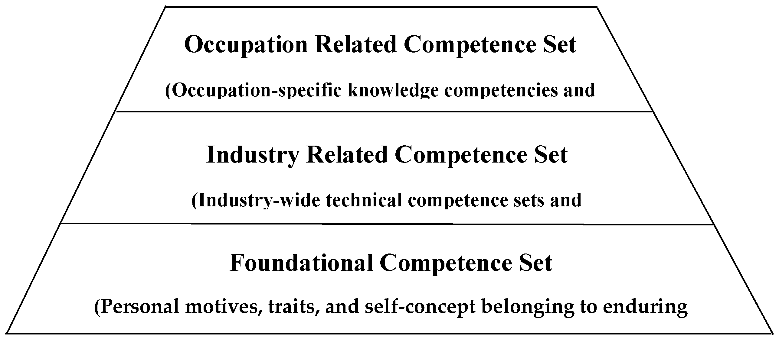
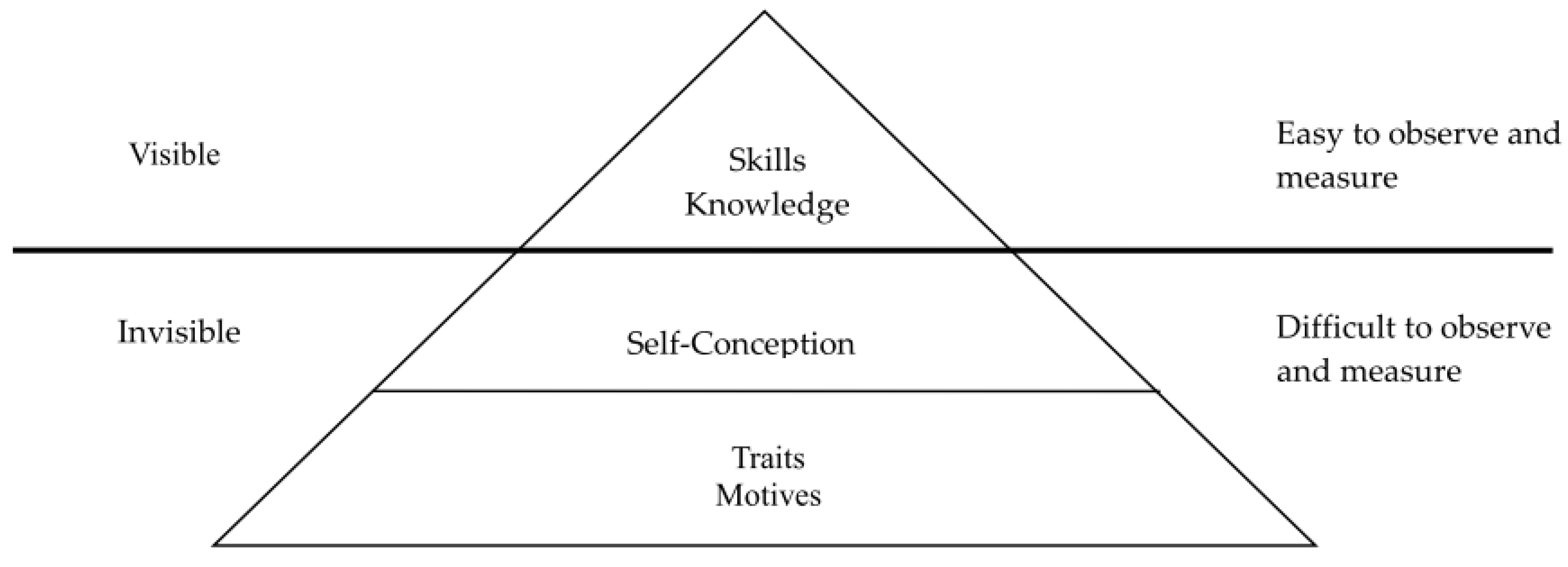
2. Review on Related Attributes in Competence Sets of Employee Capabilities

Competency was first proposed and assessed by McClelland in the early 1970s. Competencies were recognized as crucial indicators of employee performance and success as well as a person’s knowledge ability, as measured through test scores [22]. Many definitions have extended McClelland’s concept, such as the capability of applying knowledge, skills, abilities, and behaviors to successfully perform a critical task and function in a given job role. Furthermore, motivation and perceptions of work and talent are considered influential in functioning competently and successfully in a job position [23,24,25,26]. Byhanand and Moyer defined competency as behaviors related to job performance [27], separated into the following three categories: motivation competency, behavior competency, and knowledge and skills competency (Table 1). Dubois and Rothwell [28] argued that competencies such as knowledge, skills, motivation, personality, thinking patterns, feelings, and actions are personal characteristics that must be maintained to achieve satisfactory work performance. In summary, competencies are specific personal abilities related to superior performance that are common across many situations and endure for some time [10].
A competency model is a descriptive tool for identifying the competence sets a person requires to function in a specific role within a job, company, or industry. Seven to nine competence sets forming a competency group are typically required in a competency model, defined by each occupational function and job description [13,14,15,29].
The iceberg model (systems thinking), a renowned competency model proposed by Spencer and Spencer [30], divides a competence set into internal and external components parts. The internal part, the bottom of the iceberg, is unobservable and consists of self-concept, traits, and motives. The external part, the top of the iceberg, is visible and consists of knowledge and skills that can be developed through training. The iceberg model is separated into five levels, as shown in Figure 2.
The Employment and Training Administration (ETA) of the U.S. Department of Labor [31] constructed a general competency model (Figure 3) and assessed the appropriate and specific hierarchy to determine the needs of occupations in targeted industries such as nursing, process engineering, product engineering in the semiconductor industry, and computer programming in the information technology industry [8].
The ETA competency model has three tiers, with the lower tiers serving as building blocks for the higher tiers [32]. The bottom of the competency model describes the foundational competence set with a broad application to many industries or occupations. The foundational competence set includes personal motives, traits, and self-concept, which belong to enduring abilities or performance in individual growth, and these competencies develop since childhood. As a person moves up the tiers, their competence set becomes more specific to an industry and occupation. The middle tier is for industry-related competence sets including industry-wide technical competence sets and industry-specific technical competencies. The third tier of the competency model is for occupation-related competence sets, and these include occupation-specific knowledge competencies and occupation-specific technical competence sets (i.e., work ability, etc.). Because occupation- and industry-related competence sets are adapted through training (internal and external education training, and learning through teamwork), this study mainly concentrated on the middle tier of the competency model to emphasize the learning and transformation of knowledge from explicit to tacit knowledge [33]. How can the so-called “right person in the right position” situation be achieved? A competence set of personal knowledge was developed to reduce the performance gaps of components (called attributes or criteria) between learning and doing. The value of competency models is their whole-person assessment or holistic approach in examining competencies within a given occupation, and such information has been used successfully for human resource development in various applications within the workforce [1].
Because an individual competence set can be a collection of sets containing subsets of internal and external competence sets, there are two reasons for competence set expansion [14,15,17,18,19,34,35,36]. One reason is that competence set acquisition can aid the acquisition of desired skills, knowledge, behaviors, and traits through training and development. For instance, both sales persons and cashiers work with customers but require different capacities for interpersonal skills, computation, and speaking [16]. The second reason is the degree to which competencies are essential may vary depending on the job requirements of a position, and the need to expand a competence set may vary accordingly. Yu and Zhang showed that a competence set exists for each decision problem and its solution, and they used a minimal spanning tree to prove the need for competence set expansion [14,15,34].
When a competence set is perceived, decision-making becomes quick and confident. For example, an experienced used-car agency is quicker in making decisions to buy or sell cars than a novice agency is. There are different levels of proficiency for the behavioral descriptors included in a competency model, and the competence set expansion depends on whether individuals improve through experience or by learning from other people. Consequently, to expand their competence set, individuals increase their degree of competency according to their experience, and strengthen their willingness to be a lifelong learner. The Occupational Information Network (O*net) provides many official definitions of knowledge in a competence set [7]. Because the participants of the present study were marketing staff members, we referred to these definitions as employee attributes in a competence set. We selected 13 main competencies (Table 2) after consulting marketing experts. Thus, these competency definitions are referred to in this study as employee attributes in a competency set of an employee at their workplace.

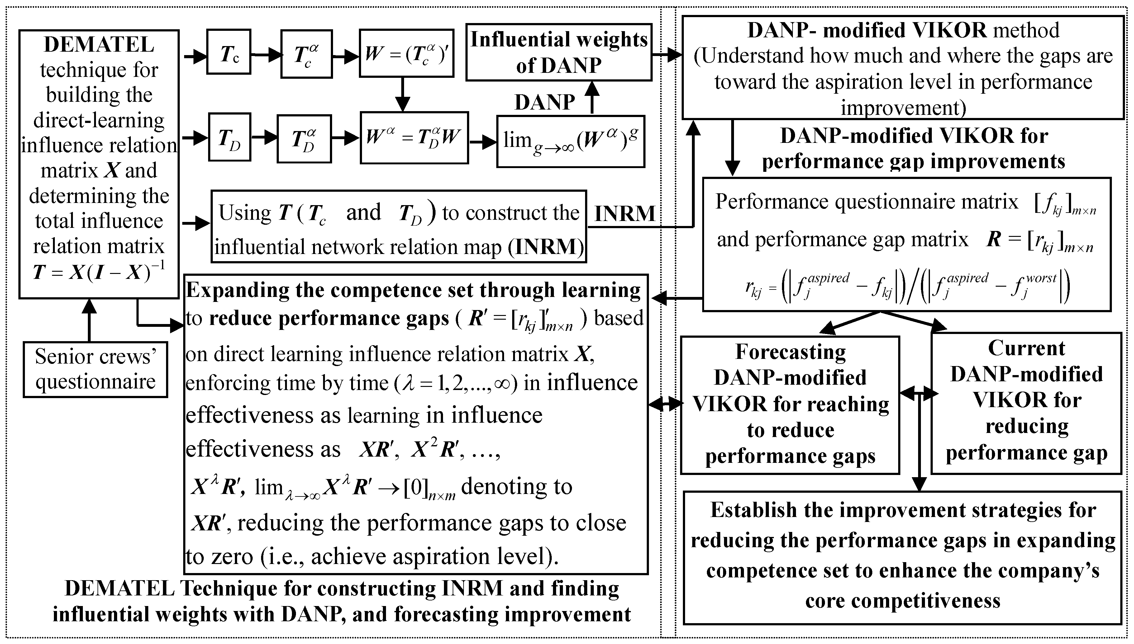
3. Hybrid MADM Model for Performance Gap Improvement

Hwang and Yoon classified multiple criteria decision-making (MCDM) problems into two main categories according to their different purposes and data types [37]: MADM and multiple objective decision-making (MODM) problems. MADM considers multiple attributes simultaneously and helps DMs evaluate, estimate, and choose the optimal alternative based on the characteristics of a limited number of cases for ranking and selection in the traditional approach [38,39,40,41,42,43,44,45,46]. MODM is typically applied in the areas of design and planning, and generally involves attempting to achieve optimal goals by considering various interactions within given constraints, such that both the decision space and objective space are changeable in new research concepts [47,48,49,50]. The present study focused on MADM; because traditional MADM ignores some critical concepts and requires some assumptions to solve actual problems (limitations and defects such as independence among criteria, probability distribution, and linearity), this study proposed a new hybrid MADM model to reduce the number of required assumptions [51] for evaluating how “competence set expansion” can be implemented in such a manner that it avoids “unrealistic assumptions in statistics and economics” [52,53,54]. The DEMATEL technique was used to construct an INRM (Section 3.1) and determine the influential weights through a DANP, which is based on the ANP (Section 3.2) [21]. A modified VIKOR method, which combines the DANP influential weights as a weighting performance-gaps for integration, was used to correct the traditional maximum–minimum as the positive and negative ideal points for the aspiration level, and the worst value for performance improvement was used to avoid simply choosing the optimum among inferior options at the aspiration level on the basis of the INRM (Section 3.3). A systematic approach to problem solving is required; instead of addressing the symptoms of a performance improvement problem, we must identify its sources to avoid “piecemeal stopgap measures”. The use of the new hybrid MADM model in performance gap improvement is illustrated in Section 3.4. Figure 4 depicts the research processes.

3.1. DEMATEL Technique for Constructing the INRM

The DEMATEL technique has been successfully used to evaluate the intertwined effects of e-learning programs [55], to identify critical success factors in adoption and assessment processes for emergencies [56], to improve radio-frequency identification adoption in Taiwan’s health care industry [45], to explore mobile banking services for user adoption intention behaviors [57], and in knowledge management [58] and information security risk control assessment [59]. This technique increases the interdependence of variables and criteria and restricts the relations that reflect characteristics in an essential systemic and developmental trend. The method is summarized in the following steps [58,60].
Step 1: Determine the initial average influence relation matrix A by assigning scores to each factor. Suppose we have n factors. Respondents (experts or stakeholders) are asked to rate the direct effects that attribute i has on attribute j by using an integer scale ranging from 0 (no influence) to 4 (very high influence). The mean score among respondents is then calculated to obtain element a i j and form the initial average influence relation matrix A = [ a i j ] n × n .
Step 2: Determine the normalized direct influence relation matrix X . From the initial average influence relation matrix A , the normalized direct influence relation matrix X = [ x i j ] n × n is calculated using Equations (1) and (2):
X = z A
z = min { 1 / max i j = 1 n a i j ,    1 / max j i = 1 n a i j } ,    i , j { 1 , 2 , , n }
Step 3: Calculate the total influence relation matrix T . total influence relation matrix T is obtained by summing the direct and indirect influences:
T = X + X 2 + X 3 + + X ρ = X ( I + X + X 2 + + X ρ 1 ) [ ( I X ) ( I X ) 1 ] = X ( I X ρ ) ( I X ) 1
where I denotes the identity matrix and ( I X ) ( I X ) 1 = I . Then,
T = X ( I X ) 1 ,   when   ρ ,   lim ρ X ρ = [ 0 ] n × n
where X = [ x i j ] n × n , 0 x i j < 1 , 0 i = 1 n x i j 1 , 0 j = 1 n x i j 1 , and at least one (but not all) of the columns or rows of the summation is equal to 1 in i = 1 n x i j and j = 1 n x i j , and thus lim ρ X ρ = [ 0 ] n × n .
We can denote the row and column sums of the total influence relation matrix T as column vectors r and s , respectively:
T = [ t i j ] n × n , i , j = 1 , 2 , , n , r = [ r i ] n × 1 = [ j = 1 n t i j ] n × 1 = ( r 1 , , r i , , r n ) ,    s = [ s j ] n × 1 = [ i = 1 n t i j ] 1 × n = ( s 1 , , s j , , s n )
where the superscript   denotes the transpose.
When i = j and i , j { 1 , 2 , , n } , if r i denotes the row sum j = 1 n t i j of the ith row of matrix T , then r i denotes the sum of the direct and indirect influences of attribute i on all other attributes. If s i denotes the column sum from matrix T , then s i denotes the sum of the direct and indirect influences that attribute i has received from all other attributes. Furthermore, ( r i + s i ) provides an index of the strength of the influences that are given and received; in other words, ( r i + s i ) shows the degree of total influences that attribute i has in this influence system. Therefore, if ( r i s i ) is positive, then attribute i has a net influence on the other attributes; if ( r i s i ) is negative, then factor i is, on the whole, being influenced by the other attributes.

3.2. DEMATEL Technique for Determining the DANP Influence Weights

The total influence relation matrix T c = [ t i j ] n × n is defined by the criteria, and T D = [ t i j D ] m × m is defined by the dimensions; T D can be obtained from T c . Next, the total influence relation matrix T c is normalized by each dimension and the influence relation matrix T D is normalized by the total row sums shown as T c α and T D α , respectively. The unweighted super-matrix W is obtained by transposing the normalized total influence relation matrix T c α in conformance with the definition of the basic concept of the ANP [21], the unweighted super-matrix W = ( T c α ) . The weighted super-matrix W α = T D α W is then obtained (i.e., the normalized super-matrix W as shown W α ). Finally, the influential weights of the DANP can be obtained by taking lim g ( W α ) g , where g represents any number as a power. The vector of influential weights w = ( w 1 , , w j , , w n ) can be then obtained, which is called the DANP. The procedures are described in the following five steps.
Step 1: Determine the total influence relation matrix for criteria T c = [ t i j ] n × n . The total influence relation matrix T c for the criteria is expressed in Equation (6), where j = 1 m m j = n , m < n , and T c i j as a m j × m j matrix.
Sustainability 08 00175 i001
Step 2: Determining the normalized total influence relation matrix for the criteria dimensions, T c α . This matrix is expressed in Equation (7).
Sustainability 08 00175 i002
As an example, an explanation for the normalization of T c α 11 on Dimension 1 based on Dimension 1 ( α 11 ) is shown in Equations (8) and (9).
T c 11 = [ t i j 11 ] m 1 × m 1 ,    t c i 11 = j = 1 m 1 t i j 11 , i = 1 , 2 , , m 1
T c 11 = [ t c 11 11 / t c 1 11 t c 1 j 11 / t c 1 11 t c 1 m 1 11 / t c 1 11 t c i 1 11 / t c i 11 t c i j 11 / t c i 11 t c i m 1 11 / t c i 11 t c m 1 1 11 / t c m 1 11 t c m 1 j 11 / t c m 1 11 t c m 1 m 1 11 / t c m 1 11 ] = [ t c 11 α 11 t c 1 j α 11 t c 1 m 1 α 11 t c i 1 α 11 t c i j α 11 t c i m 1 α 11 t c m 1 1 α 11 t c m 1 j α 11 t c m 1 m 1 α 11 ]
where t c i j α 11 = t c i j 11 / t c i 11 denotes the element of the normalized influence for element t c i j 11 as a scalar (showing the influence of element of attribute i on other criteria j ( j = 1 , 2 , , m 1 ) , in which Dimension 1 influences Dimension 1 of the total influence relation matrix) divided by the sum t c i 11 ( t c i 11 = j = 1 m 1 t i j 11 , i = 1 , 2 , , m 1 ) of each row (attribute i influences all other attributes in Dimension 1).
Step 3: Determine the unweighted super-matrix W by transposing the normalized total influence relation matrix T c α . Because the total influence relation matrix T c matches and fills the interdependence or interrelationship among the dimensions and attributes, the normalized total influence relation matrix T c α can be transposed by the dimensions, based on the basic concept of the ANP [21], resulting in the unweighted super-matrix W = ( T c α ) , as shown in Equation (10).
Sustainability 08 00175 i003
Step 4: Determine the weighted super-matrix W α . The weighted super-matrix W α (called the normalized super-matrix) is obtained from the unweighted super-matrix W by multiplying T D α (i.e., W α = T D α W ). The normalized total influence relation matrix T D α can be obtained by applying to normalize the total influence relation matrix T D = [ t D i j ] m × m in the process, as shown in Equation (11), where t D i j is a scalar (element) and i , j { 1 , 2 , , m } .
T D = [ t D 11 t D 1 j t D 1 m t D i 1 t D i j t D i m t D m 1 t D m j t D m m ]
We normalized the total influence relation matrix T D of the dimensions (i.e., Equation (11)) and obtained a new normalized total influence matrix T D α of the dimensions, as shown in Equation (12).
T D α = [ t D 11 / d 1 t D 1 j / d 1 t D 1 m / d 1 t D i 1 / d i t D i j / d i t D i m / d i t D m 1 / d m t D m j / d m t D m m / d m ] = [ t D α 11 t D α 1 j t D α 1 m t D α i 1 t D α i j t D α i m t D α m 1 t D α m j t D α m m ]
where T D α = [ t D α i j ] m × m , t D α i j = t D i j / d i , and d i = j = 1 m t D i j .
Next, the normalized total influence relation matrix of dimension T D α is multiplied with the unweighted super-matrix W to obtain a new weighted super-matrix W α (i.e., by the normalized matrix), as shown in Equation (13), where t D α i j is a scalar and j = 1 m m j = n .
Sustainability 08 00175 i004
Step 5: Determine the limits of the weighted super-matrix W α by raising it to a sufficiently large power. If the weighted super-matrix W α is raised to a sufficiently large power g , then the weighted normalized super-matrix W α converges and becomes a long-term stable super-matrix (using the basic concept of a Markov chain). In other words, lim g ( W α ) g , where g represents any number as a power. Consequently, what the DANP calls the “vector of influential weights” (i.e., global influential weights) as w = ( w 1 , , w j , , w n ) is obtained. To visualize the complex co-influenced relationships between competences on a visible and precise map, the INRM is used with the value of ( r i + s i ) and ( r i s i ) representing the x- and y-axes, respectively [52,53].

3.3. Modified VIKOR Method for Ranking and Improving Competence Sets

Opricovic [61] proposed implementing the compromise-ranking VIKOR method within the MADM model [38,39,40,41,42,43,44]. If the feasible alternatives are represented by A 1 , , A k , , A K , then the performance scores of alternative A k in each criterion j can be denoted as f k j ( k = 1 , 2 , , K ; j = 1 , 2 , , n ); w j uses the influential weight (by the DANP) of the jth criterion, where j = 1 , 2 , , n , and n is the number of criteria. We define the best f j a s p i r e d values, called “aspiration level” by Simon [62,63], and the worst f j w o r s t values of all the criteria, j = 1 , 2 , , n . We begin developing the modified VIKOR method by using the following form as the L p - metric :
L k p = { j = 1 n [ w j ( | f j a s p i r e d f k j | ) / ( | f j a s p i r e d f j w o r s t | ) ] p } 1 / p
where 1 p ; k = 1 , 2 , , K ; the weight w j is derived from the DANP. To formulate the ranking and gap measures, L k p = 1 (as E k ) and L k p = (as Q k ) are used in the basic concept of the traditional VIKOR method [39,40,41,42,43,44,61], as shown in Equations (15) and (16).
L k p = { j = 1 n [ w j ( | f j f k j | ) / ( | f j f j | ) ] p } 1 / p
L k p = 1 = j = 1 n [ w j ( | f j f k j | ) / ( | f j f j | ) ]
L k p = = max j { ( | f j * f k j | ) / ( | f j * f j | ) | j = 1 , 2 , , n }
where f j * = max k { f k j | k = 1 , 2 , , K } and f j = min k { f k j | k = 1 , 2 , , K } form the traditional approach. Equations (15) and (16) are then rewritten as Equations (17) and (18):
E k = L k p = 1 = j = 1 n [ w j ( | f j a s p i r e d f k j | ) / ( | f j a s p i r e d f j w o r s t | ) ]
Q k = L k p = = max j { ( | f j a s p i r e d f k j | ) / ( | f j a s p i r e d f j w o r s t | ) | j = 1 , 2 , , n }
The compromise solution min k L k p shows that the synthesized and integrated gap is the minimum; consequently, it is ranked and selected, and is improved so that its value is as close as possible to the aspirational level. In addition, the group utility (called the average gap or average degree of regret) is emphasized when the value of p is low (such as p = 1 ); however, if p is infinite (i.e., p = ), then the individual maximum regrets and gaps gain prominence in prior improvements. In other words, it is shown by minimizing average gap; however, the min k Q k stresses selecting the minimum from the maximum individual regrets and gaps (shown by the maximum gap for prior improvement) in the basic concept of the DANP-modified VIKOR method. The compromise-ranking and improvement DANP-modified VIKOR method entails three steps, as follows.
Step 1: Obtain the aspirational level and the worst value. The best f j a s p i r e d values (called the aspiration level by Simon [62,63], which Simon incorporated into his work, receiving the Nobel Prize in Economics in 1978) and worst f j w o r s t values are calculated for all criterion functions, j = 1 , 2 , , m . The performance value of each criterion can be obtained using questionnaires with a scale ranging from 0 (complete dissatisfaction) to 10 points (complete satisfaction). Therefore, the aspiration level is set as f j a s p i r e d = 10 and the worst value as f j w o r s t = 0 . In this study, we set f j a s p i r e d = 10 as the aspiration level and f j w o r s t = 0 as the worst value for normalization; this is in contrast to the traditional approach, which sets f j * = max k { f k j | k = 1 , 2 , , K } and f j = min k { f k j | k = 1 , 2 , , K } as the aspiration level and worst value, respectively. We proposed this new idea to avoid “the traditional approach of choosing the optimum among inferior alternatives”, in the other words, to avoid “selecting the best option among a list of poor options”. Thus, the original maximum–minimum performance-rating matrix can be converted into a normalized gap-rating matrix [ r k j ] m × n by using the aspiration level ( f j a s p i r e d ) and worst value ( f j w o r s t ), r k j , as shown in Equation (19).
r k j = ( | f j a s p i r e d f k j | ) / ( | f j a s p i r e d f j w o r s t | ) ,    k = 1 , 2 , , K   and   j = 1 , 2 , , n ,
where the rating r k j shows the gap of alternative k in criterion j . Next, we must determine how to leverage innovation and creativity through systematic consideration to reduce all performance gaps in the criteria and dimensions, and overall, to approach zero (i.e., toward the aspiration level), based on the INRM.
Step 2: Calculate the means of the group utility and maximal regret. These gap values can be computed using the rating-weighted S k = j = 1 n w j r k j (i.e., the synthesized and integrated gap for all criteria to reduce the gaps of each criterion or attribute to approach zero by leveraging systematic innovation or creativity) and Q k = max j { r k j | j = 1 , 2 , , n } (shown by the maximal gap of alternative k, in which criterion j as prior improvement for each dimension and overall, respectively).
Step 3: Calculate the index value. This value can be measured using the following Equation:
U k = σ ( E k E * ) / ( E E * ) + ( 1 σ ) ( Q k Q * ) / ( Q Q * ) ,    σ [ 0 , 1 ]
where E * = min k E k following the traditional approach, or E * = E a s p i r e d = 0 (no gap; the aspiration level is achieved) using our approach; E = max i E i following the traditional approach, or E = E w o r s t = 1 (the worst situation) using our approach; Q * = min k Q k following the traditional approach, or Q = Q a s p i r e d = 0 (no gap; the aspiration level is achieved) using our approach; and Q = max k Q k following the traditional approach, or Q w o r s t = 1 (the worst situation) using our approach. Therefore, Equation (20) can be rewritten as U k = σ E k + ( 1 σ ) Q k , where E = E a s p i r e d = 0 and Q = Q a s p i r e d = 0 (i.e., all the attributes have achieved their corresponding aspiration levels), and E = E w o r s t = 1 and Q = Q w o r s t = 1 (i.e., the worst situation).
The means for DMs to determine the σ value is described as follows. When σ = 1 , only the average gap (average regret) is considered in each dimension or overall; when σ = 0 , only the maximum gap in improvement is considered a priority for the criterion of each dimension or overall. The value obtained from min S k represents the maximum group utility (the minimum average gap indicator) of competence k, and the value obtained from maximal Q k represents the maximum regret of competence k (the largest gap shown as a priority improvement). Thus, v represents the weight of the strategy. Generally, σ = 5 , and can be adjusted depending on the case for improvement priority; σ = 1 indicates that only the average gap is considered, and σ = 0 indicates that only the maximum gap is prioritized for individual improvement.
The VIKOR method was applied to determine the compromise solution according to measured gaps. This solution is useful for DMs because it offers the maximum group utility for the majority (shown by the minimal E k ; i.e., minimizing the average gap in competence k) and the maximum regret for the minimum number of individuals of the opponent (shown by the minimum Q k ; i.e., the maximum gap for priority improvement in competence k).

3.4. Performance Gap Improvement for Establishing Improvement Strategies

The hybrid MADM model can be used to apply performance gap improvements by determining the causal criteria and by suggesting a strategy for innovation and creativity in interrelationship among the criteria. Using the normalized direct-learning influence relation matrix X = [ x i j ] n × n to know (i.e., forecast) how much change to improve or reduce the performance gap of each criterion in influential relationship is described as follows. To improve the performance gap r k j in continuous learning, the performance gaps in the modified VIKOR matrix R = [ r k j ] m × n , where r k j = ( | f j a s p i r e d f k j | ) / ( | f j a s p i r e d f j w o r s t | ) , k = 1 , 2 , , K , and j = 1 , 2 , , n , adopt the normalized direct-learning influence relation matrix X = [ x i j ] n × n ( 0 x i j < 1 , 0 i = 1 n x i j 1 , 0 j = 1 n x i j 1 , and at least one, but not all, of the columns or rows of the summation is equal to 1 in i = 1 n x i j and j = 1 n x i j ) for the performance gap matrix R = [ r k j ] K × n in each iteration of the improvement-learning period. In other words, the direct-learning influence relation matrix (i.e., learning time by time) can be reduced to X R , X 2 R ,…, X λ R ,…; where X λ R (as lim λ X λ R = [ 0 ] n × K , because lim λ X λ = [ 0 ] n × n ) denotes improvement in the performance gap matrix R = [ r k j ] K × n (i.e., R = [ r k j ] K × n = [ r j k ] n × K , where the superscript denotes the transpose). The net results of all improvement-learning periods are as follows.
G n e t g a p ( n × K ) ( 0 ) = X 0 R = R G n e t g a p ( n × K ) ( 1 ) = X G n e t g a p ( n × K ) ( 0 ) = X R G n e t g a p ( n × K ) ( 2 ) = X G n e t g a p ( n × K ) ( 1 ) = X ( X R ) = X 2 R G n e t g a p ( n × K ) ( λ ) = X G n e t g a p ( n × K ) ( λ 1 ) = X ( X λ 1 R ) = X λ R
For the simplicity of formulation, G n e t g a p ( n × K ) ( λ ) satisfies the iteration function:
V λ ( R ) = min n e t g a p { X G n e t g a p ( n × K ) λ 1 } ,    where    λ = 1 , 2 , , .
A longitudinal survey must be administered to measure real performance. Equation (21) can be viewed as an initial forecasting technique for providing a reference for DMs as well as a recommendation of which performance or effect should be improved as a first priority. This technique reduces recollection and resurvey costs and causes an expected effect while implementing improvements; thus, Equation (21) is implemented at a sufficiently large power λ until the net-gap learning performance approaches the zero matrix [ 0 ] n × K (i.e., G n e t g a p ( n × K ) ( λ ) = l i m λ X λ R = [ 0 ] n × K ). This learning result could satisfy approaching the aspiration level in a competence set expansion.
In this empirical case, we use an example where λ = 0 , λ = 10 , λ = 20 , …; the total average performance-learning gap of V λ ( R ) can be obtained using w G n e t g a p ( n × K ) λ and λ = 0 , 1 , , ; where vector w = ( w 1 , , w j , w ) n is the influential weights of the DANP. We apply the iteration learning idea (based on the input–output table by Leontief [64,65,66]. to obtain an expected performance for DMs to understand the gap between the ordinal and forecasting values after computing two progressions of the proposed model. In addition, the expected performance level (near the aspiration level; i.e., the performance gap matrix R = [ r k j ] K × n approaching the zero matrix [ 0 ] K × n ) derives from the outcome of iterative learning between all criteria. This not only considers the criteria influencing the INRM, but also determines the extent to which the performance of the DANP-modified VIKOR can change.

4. Empirical Case for Enhancing a Company’s Core Competitiveness

In this study, we applied the proposed model to an empirical case with the aim of enhancing a company’s core competitiveness. Section 4.1 briefly presents the problem, Section 4.2 describes the results and analyses, and a discussion and the implications are presented in Section 4.3. We surveyed the marketing department of Warehouse Store H using two questionnaires. The first questionnaire was administered to 14 senior staff members as representative experts in building the influential relationships of the competencies as the criteria described in Section 2. The second questionnaire was administered to employees who acknowledged the performance so far. The goal of this study was to provide critical marketing competencies for managers to establish an effective business education or apprenticeship program by reducing or eliminating the gaps between staff abilities and aspiration levels.

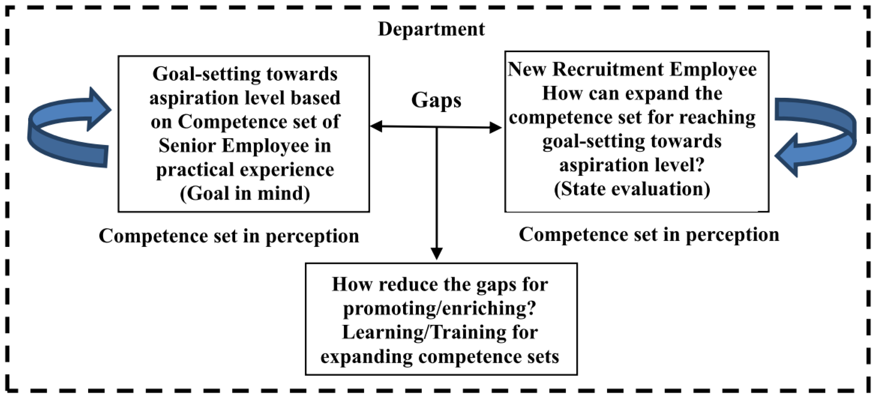
4.1. Problem Description

Warehouse Store H is a local shopping mall established in 2000 and has directly managed branches only in the south of Taiwan. The store wanted to improve its competiveness to open new branches in the northern areas of Taiwan such as in Hsinchu, Taoyuan, and Taipei. However, its external challenge was in facing other warehouse stores, such as Costco, Carrefour, and RT-Mart, which had massive cost advantages creating high entry barriers to the business. The company’s internal challenge was that it had always used traditional marketing approaches such as leafleting, bundle selling, and sales promotion during festivals such as Christmas and the mid-autumn festival. Even if H duplicated the marketing techniques of other warehouse stores, it would still lack the price competiveness required to attract more customers and the capital necessary to create mass sales events to increase income. Challenges will always exist, both internally and externally; H should first resolve its internal problems to strengthen internal self-competiveness and opportunities before considering external weaknesses and threats to improve the competiveness of the company as a whole.
This study first inspected the internal marketing department of Warehouse Store H to determine the reason it cannot implement a more effective marketing approach compared with its competitors. We surveyed the marketing department of H by using two questionnaires. The first questionnaire was administered to 14 senior staff members to build the influential relationships of the competencies, as described in Section 2. The second questionnaire was administered to the employees who had acknowledged the performance so far. According to the study goal, the significant confidence f the total influence relation matrix T c was verified by consensus; the test results of the significant confidence reached 96.88% in consensus by the senior staff members, φ = 14. When the total influence relation matrix T c ( n × n matrix), the average gap-ratio = ( 1 / n 2 ) i = 1 n j = 1 n ( | t i j φ t i j φ 1 | / t i j φ ) × 100 % = 3.12 % < 5 % , significant confidence reach 96.88% in consensus, where φ = 14 and φ 1 = 13 denote the number of experts (senior employee) in practical experience and t i j φ is the average influence of criterion i on criterion j in φ number of experts (senior employee), and n denotes the number of criteria; here n = 13 and the matrix is n × n .

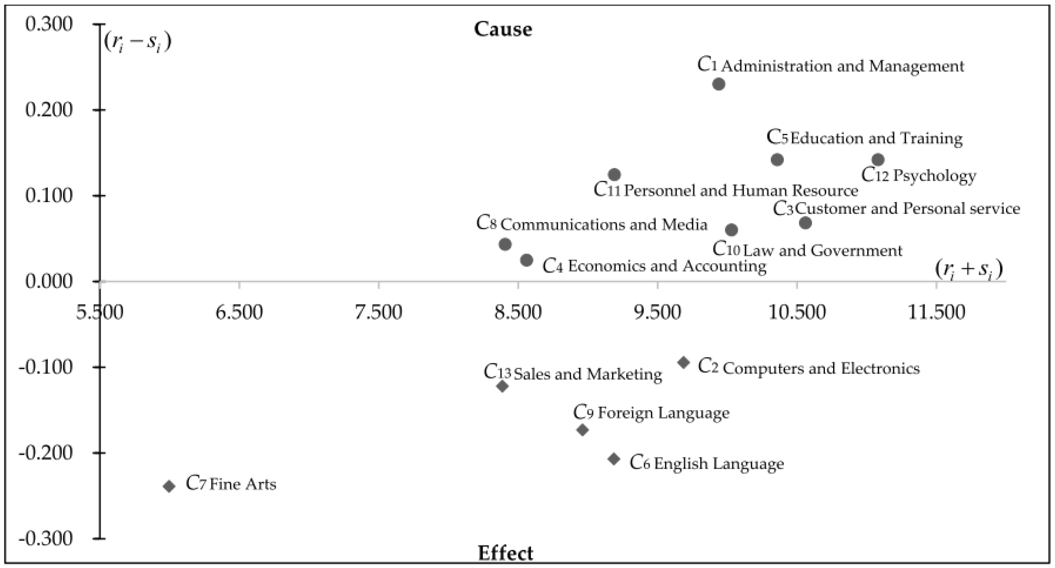
4.2. Results and Analysis

DEMATEL technique for constructing the INRM and determining the DANP influential weights. To construct an INRM, the DEMATEL technique was adopted to construct the influential relationships among the criteria by using pair-wise comparisons (Figure 5). This technique can help DMs determine the priority for improving their current key concerns. The participants (i.e., the members of H’s marketing department) were asked to determine the influence of the relationships between the criteria in the first questionnaire.
As matrix X shows, the normalized direct influence relation matrix X  was calculated using Equations (1) and (2), and is shown in Table 3. The total influence relation matrix T c was then derived using Equations (3), (6), and (9), and is shown in Table 4. Furthermore, Equations (4) and (5) were used to summarize the total influence given and received according to each dimension and criterion (Table 5). Thus, the INRM of the DEMATEL technique can be implemented as shown in Figure 4 by using the net INRM in Table 5.
As shown in Table 5, we obtained the INRM (Figure 5). Figure 5 shows that the ( r i s i ) of C 1 (Administration and Management) was the highest net influence competency, the ( r i + s i ) of C 12 (Psychology) showed the largest degree of co-influence competencies, C 1 was the greatest co-influence cause in this system, and C 7 (Fine Arts) exerted the smallest competency effect. Consequently, we divided the cause and effect competencies into two sets and computed the distance between them.

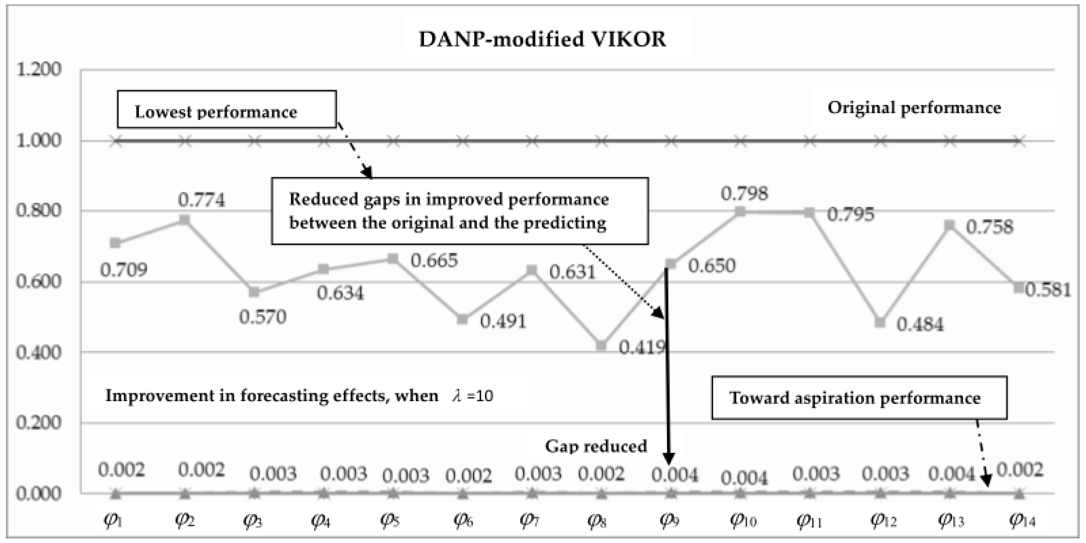
Performance of Competence Sets Determined Using the DANP-Modified VIKOR Method

The second questionnaire was on competency performance and was administered to 14 participants. This questionnaire used an 11-point scale ranging from 0 (very poor performance) to 10 (excellent performance). We set f j a s p i r e d = 10 as the aspiration level and f j w o r s t = 0 as the worst value. By using the DANP-modified VIKOR method, it was hoped that DMs could improve and train employees to expand their competence sets and that new recruiters could use the results while providing apprenticeships (i.e., experienced employees guiding new employees to enhance competence sets). The influential weights of the DANP were obtained by limiting the power of the weighted super-matrix ( lim g ( W α ) g ) until it reached a steady state (Table 6). Note that C 1 (Administration and Management) had the highest influential weight 0.0836 and C 13 (Sales and Marketing) had the lowest influential weight 0.0727.
Table 7 shows the outcome of the DANP-modified VIKOR method and the average gap or regret of each object E k ( k = 1 , 2 , , 14 ) , the maximal gap or regret of each object Q k ( k = 1 , 2 , , 14 ) , and the synthesizing E k and Q k index of each object U k in competence set performance, according to Equations (14)–(20). This study collected the empirical questionnaire from the marketing department of H warehouse store.
After normalizing the values shown in Table 7, the outcome of the performance gap for the participants was precisely illustrated. The performance gap r k j = ( | f j a s p i r e d f k j | ) / ( | f j a s p i r e d f j w o r s t | ) (i.e., Equation (18)) represents relative values in competence f k j for participant φ k ; f k j is the performance value in each competence C j , j = 1 , 2 , , 13 for participant φ k , k = 1 , 2 , , 14 ; and f j a s p i r e d = 10 and f j w o r s t = 0 are the aspiration level and the worst performance value, respectively. The rank of participants is illustrated in Figure 6, with φ 8 showing outstanding work performance for his or her individual competences and φ 10 showing the lowest performance in this study. However, φ 1 (Fine Arts) was affected by the cause competences (i.e., C 1 , C 3 , C 4 , C 5 , C 8 , C 10 , C 11 , and C 12 ). Moreover, the most influenced competencies, C 1 (Administration and Management) and C 12 (Psychology), represented the cause competence gaps between φ 8 and φ 10 . Therefore, to expand the competence set of X , φ 8 should teach φ 10 or they should work together.

4.3. Discussion and Implications

As shown in Figure 5, values above the x-axis lines are causal competences that, if improved, would have a gearing improvement according to the DEMATEL technique. By applying Equation (22), we evaluated the effect of the performance such that obtaining the forecasting performance by λ = 1 , 2 , , 50 would become stable and the overall performance would improve to excellent (see the Appendix A for the computation of the forecasting performance). Table 8 shows the forecasting performance when the DANP-modified VIKOR method was used with λ = 10 (see Appendix A Table A4, Table A5, and Table A6 for λ = 20 , λ = 40 , and λ = 50 , respectively). Because each person is limited by different abilities, skills, and willingness to change, strategies to improve individual competencies should be established through different means.
Table 9 shows that the rank of the participants changed with the forecasted results; for example, φ 14 increased from Rank 5 to Rank 2 because of a change in V λ ( R ) resulting from the competencies’ co-influenced weights. Performance was improved by increasing the co-influence weights, resulting in the individuals’ competence sets reaching satisfactory levels if having the direct and focus on competence to enhance, as Figure 6 shows that the improvement effort was substantial and proximal to the aspiration level.

5. Conclusions and Remarks

In this study, we obtained the expected and forecast performance to improve an individual’s competence set by applying a DANP-modified VIKOR method with a net influence value. Staff performance was improved by improving their competence sets. In addition, an individual could expand his or her competence set to break both competence sets while improving individually with each set; this is the so-called “competence set expansion” from habitual domain theory, which was proposed by Yu [67,68]. Using the proposed model, we determined that the critical competencies of C 1 (Administration and Management), C 3 (Customer and Personal Services), C 4 (Economics and Accounting), C 5 (Education and Training), C 8 (Communications and Media), C 10 (Law and Government), C 11 (Personnel and Human Resources), and C 12 (Psychology) influenced the affected competencies of C 2 (Computers and Electronics), C 13 (Sales and Marketing), C 9 (Foreign Languages), C 6 (English Language), and C 7 (Fine Arts). Whole individual abilities were improved (i.e., competence set expansion), resulting in a change in the original performance rank. The competence sets might have improved incrementally over time through learning by doing. Therefore, the predicting performance is expected to indicate how much improvement can be achieved after a period, which is not to jump to the expectation the performance will improve once a period.
The proposed model was applied to data collected from Warehouse Store H. We anticipate that DMs can recognize the advantages and weaknesses of each person’s competencies as well as the gap between individuals, such that performance can be improved (i.e., by reducing the gap) toward the aspiration level, either by using internal business education or by having experienced employees mentor new employees. Although each employee has specific talent limitations, continuous promotion in human resources management remains an effective method for improving overall business operations in the face of high competition.
One of the main contributions of this study is that it provides the criteria for a forecasting technique as an iterative function for DMs to use as a reference in predicting performance. After H improved the criteria, we would be able to estimate the anticipated improvement to show the DMs that if H follows the progress of the proposed model, then the whole department gap would decrease to a reasonable level, after which a decision to change the present situation could be made. However, this technique cannot replace real data; if the technique is repeated without implementing an improvement plan, the results might not reflect real performance and the effect of the improvement plan might not be realized. Therefore, we recommend that this prediction technique be implemented between two improvement plans (original performance and toward the aspiration level by improving the predictive effect, when λ = 10 , as the example case shows in Figure 6) for continuous improvement through the following steps: (1) survey the current situation; (2) apply the proposed model to compare the effect; (3) implement an improvement plan according to an evaluation of the expected effect from forecasting; and (4) re-collect the improved data and reiterate the proposed model. The technique always has bias toward real world situations between theoretical predictions and practical complements in each other. Thus, it will result in an imbalance and variance between theory and practice.
We suggest several areas for expanding this study: (1) applying MODM methods to redesign the changeable space of the competence set for the expansion of each participant, and adding some constraints such as efficient time usage, individual talents, and learning curves; (2) reducing or combining unnecessary competencies by applying MODM programming; and (3) considering marketing department performance; thus, if a weaker employee can learn from another’s stronger ability, the rank will be changed and the weaker employee’s competence expanded. In other words, if all lower-ranked employees could improve their weaknesses and strengthen their advantages, the MCDM model (MADM + MODM) would develop more completely.
Finally, the aspiration level could have been limited by the questionnaire or by the current environment. Determining whether theoretical or practical limits exist for the aspiration levels will require considerable effort.

Acknowledgments

The authors are grateful to helpful suggestions and comments made by anonymous reviewers on an earlier version of the paper. We also thank Ministry of Science and Technology (Grant MOST 104-2410-H-305 -052 -MY3) for its financial support.

Author Contributions

Kuan-Wei Huang and Gwo-Hshiung Tzeng designed the research; Jen-Hung Huang provided the research idea concept the purpose; Kuan-Wei Huang and Gwo-Hshiung Tzeng collected and analyzed the data; Kuan-Wei Huang wrote the paper; finally, Gwo-Hshiung Tzeng revised the paper. All authors have read and approve the final manuscript.

Conflicts of Interest

The authors declare no conflict of interest.

Appendix A

Forecast competence performance method
Step 1. Normalize the direct influence relation X
Table A1. Matrix X= [ x ij ] n×n .
Competence set C 1 C 2 C 3 C 4 C 5 C 6 C 7 C 8 C 9 C 10 C 11 C 12 C 13
C 1 0.0000.0980.0940.0580.0830.0770.0410.0600.0730.0810.0670.0830.074
C 2 0.0830.0000.0830.0650.0790.0710.0410.0670.0610.0770.0500.0920.067
C 3 0.0900.0920.0000.0580.0900.0770.0430.0750.0690.0790.0830.0980.081
C 4 0.0560.0730.0630.0000.0690.0650.0500.0580.0670.0600.0540.0810.054
C 5 0.0830.0770.0920.0690.0000.0880.0520.0700.0770.0860.0750.0900.069
C 6 0.0630.0600.0730.0650.0860.0000.0450.0690.0650.0730.0610.0750.050
C 7 0.0380.0470.0380.0380.0440.0400.0000.0430.0380.0330.0450.0580.033
C 8 0.0630.0670.0710.0610.0760.0730.0380.0000.0490.0660.0520.0650.054
C 9 0.0670.0630.0670.0710.0670.0560.0460.0540.0000.0750.0690.0770.056
C 10 0.0770.0830.0900.0630.0770.0670.0360.0580.0770.0290.0810.0810.060
C 11 0.0750.0480.0900.0540.0670.0670.0430.0560.0790.0810.0000.0900.060
C 12 0.0830.0940.0940.0860.1000.0880.0580.0740.0850.0750.0860.0000.077
C 13 0.0710.0540.0700.0560.0600.0520.0460.0430.0560.0560.0690.0830.000
Step 2. Adopting Equations (13)–(15) and transpose R = [ r k j ] m × n = [ r j k ] n × m to estimate the performance of the modified VIKOR
Table A2. Matrix R .
Competence
set
Participants
φ 1 φ 2 φ 3 φ 4 φ 5 φ 6 φ 7 φ 8 φ 9 φ 10 φ 11 φ 12 φ 13 φ 14
C 1 0.1000.1000.4000.3000.5000.3000.3000.3000.7000.7000.5000.4000.5000.200
C 2 0.0000.8000.7000.2000.5000.3000.3000.3000.5000.4000.5000.4000.6000.300
C 3 0.2000.2000.3000.2000.5000.3000.2000.2000.5000.5000.2000.3000.7000.100
C 4 0.3000.3000.7000.8000.5000.5000.6000.5000.7000.9000.7000.5000.5000.300
C 5 0.4000.4000.4000.5000.4000.3000.6000.3000.7000.7000.3000.5000.8000.300
C 6 0.5000.5000.5000.8000.5000.5000.5000.3000.4000.4000.7000.5000.9000.300
C 7 1.0001.0000.4000.5000.8000.3000.8000.5000.7001.0000.9000.5000.6000.300
C 8 0.8000.8000.5000.8000.7000.6000.5000.3000.7000.5001.0000.5000.4000.800
C 9 0.9000.9000.4000.5000.5000.5000.5000.4000.7000.6000.7000.5000.5000.500
C 10 0.0000.9000.4000.5000.5000.4000.5000.3000.7000.5000.5000.5000.3000.300
C 11 0.0000.0000.3000.3000.5000.3000.5000.2000.5000.5000.5000.5000.8000.500
C 12 0.7000.7000.3000.2000.5000.3000.3000.4000.7000.6000.6000.5000.7000.200
C 13 0.6000.6000.4000.5000.5000.4000.4000.4000.3000.4000.6000.5000.7000.700
E k
(average gap)
0.4180.5480.4410.4690.5300.3830.4610.3390.6000.5960.5890.4680.6170.363
Step 3. Calculate the total influence relation matrix by using X G n e t g a p ( λ 1 ) , λ = 1 , 2 , , at a sufficiently large power X λ R [ 0 ] n × m
Table A3. XR.
Table A3. XR.
Competence
set
Participants ( φ 1 )
φ 1 φ 2 φ 3 φ 4 φ 5 φ 6 φ 7 φ 8 φ 9 φ 10 φ 11 φ 12 φ 13 φ 14
C 1 0.36510.36510.39170.40710.46050.34180.39910.29340.51780.49550.50340.41590.56220.3272
C 2 0.36560.36560.34520.39980.43580.32470.37810.28070.51050.49840.48250.39310.51550.2992
C 3 0.38320.38320.41610.43890.48640.35980.43110.31720.56400.53990.56290.44930.57620.3620
C 4 0.32410.32410.31440.32480.39470.28020.33060.24350.44590.42060.43120.34950.47200.2735
C 5 0.37310.37310.40510.42280.49360.36170.40200.30950.54680.52750.55490.42960.56060.3357
C 6 0.31600.31600.33750.34550.41120.29450.35460.26310.49070.47380.44440.36560.46520.2868
C 7 0.18940.18940.21770.22430.25170.19120.21240.16070.29530.27670.28110.23140.30980.1826
C 8 0.26570.26570.32090.32380.37130.26910.32690.24480.43300.43070.39470.34030.47040.2353
C 9 0.27290.27290.33710.34900.40190.28510.34450.25350.45860.45240.43460.35760.47770.2658
C 10 0.35330.35330.38270.38810.45420.33140.38310.28820.52040.50830.49600.40550.56020.3145
C 11 0.35990.35990.34890.37470.42240.31390.35440.27630.49530.47590.46480.37470.48720.2763
C 12 0.37680.37680.45220.48420.52220.38920.46470.32700.58800.58260.57150.46350.61800.3749
C 13 0.27680.27680.30670.31320.37440.26610.32080.23520.44700.43290.40600.33150.44260.2319
E k
(average gap)
0.32530.43850.35190.36900.42170.30850.36170.26870.48560.47010.46400.37770.50130.2901
Table A4. X 20 R .
Table A4. X 20 R .
Competence
set
Participants ( λ = 20 )
φ 1 φ 2 φ 3 φ 4 φ 5 φ 6 φ 7 φ 8 φ 9 φ 10 φ 11 φ 12 φ 13 φ 14
C 1 0.00920.00920.00990.01040.01190.00870.01020.00760.01370.01330.01310.01070.01410.0082
C 2 0.00870.00870.00940.00990.01130.00820.00970.00720.01300.01260.01240.01010.01340.0077
C 3 0.00960.00960.01040.01090.01250.00910.01070.00790.01430.01390.01370.01110.01480.0086
C 4 0.00780.00780.00840.00880.01010.00740.00860.00640.01160.01120.01110.00900.01200.0069
C 5 0.00950.00950.01030.01080.01230.00900.01060.00780.01420.01370.01350.01100.01460.0085
C 6 0.00810.00810.00880.00930.01060.00770.00910.00670.01210.01180.01160.00940.01250.0073
C 7 0.00520.00520.00570.00590.00680.00500.00580.00430.00780.00750.00750.00610.00800.0047
C 8 0.00770.00770.00830.00870.00990.00730.00850.00630.01140.01110.01090.00890.01180.0068
C 9 0.00800.00800.00860.00900.01030.00760.00890.00660.01190.01150.01140.00920.01230.0071
C 10 0.00910.00910.00990.01040.01180.00860.01010.00750.01360.01320.01300.01060.01400.0081
C 11 0.00840.00840.00910.00960.01090.00800.00940.00700.01260.01220.01200.00980.01300.0075
C 12 0.01010.01010.01100.01150.01310.00960.01130.00840.01510.01460.01440.01170.01560.0090
C 13 0.00750.00750.00810.00850.00970.00710.00830.00620.01120.01080.01070.00870.01150.0067
E k
(average gap)
0.00840.01130.00910.00950.01090.00790.00930.00690.01250.01210.01190.00970.01290.0075
Table A5. X 40 R .
Table A5. X 40 R .
Competence
set
Participants ( λ = 40 )
φ 1 φ 2 φ 3 φ 4 φ 5 φ 6 φ 7 φ 8 φ 9 φ 10 φ 11 φ 12 φ 13 φ 14
C 1 0.19440.26190.21070.22110.25230.18460.21660.16080.29030.28140.27770.22580.29970.1737
C 2 0.18390.24780.19930.20920.23860.17460.20490.15210.27460.26620.26270.21360.28350.1643
C 3 0.20340.27410.22050.23140.26400.19320.22670.16830.30380.29450.29060.23630.31360.1818
C 4 0.16440.22150.17820.18700.21330.15610.18320.13600.24550.23800.23490.19100.25340.1469
C 5 0.20110.27090.21790.22870.26090.19090.22410.16630.30030.29100.28720.23360.31000.1797
C 6 0.17240.23230.18690.19620.22380.16380.19220.14260.25750.24960.24630.20030.26580.1541
C 7 0.11060.14900.11990.12580.14350.10500.12320.09150.16510.16010.15800.12850.17050.0988
C 8 0.16230.21870.17600.18460.21070.15420.18090.13430.24240.23500.23190.18860.25020.1451
C 9 0.16860.22720.18280.19180.21880.16010.18790.13940.25180.24410.24090.19590.25990.1507
C 10 0.19310.26010.20930.21960.25060.18330.21520.15970.28830.27950.27580.22430.29760.1725
C 11 0.17850.24050.19350.20300.23160.16950.19890.14760.26660.25840.25500.20740.27520.1595
C 12 0.21430.28880.23230.24380.27810.20350.23880.17720.32000.31020.30620.24900.33040.1915
C 13 0.15840.21340.17170.18020.20560.15040.17650.1310.23650.22930.22630.1840.24420.1415
E k
(average gap)
0.17740.23900.19220.20170.23020.16840.19760.14670.26480.25670.25340.20600.27340.1585
When λ = 50 , the relation matrix X G n e t g a p ( λ 1 ) from using Equation (21) (i.e., the iteration function V λ ( R ) ) yields the minimum forecasting performance improvement required to reach the aspiration level.
Table A6. X 50 R .
Table A6. X 50 R .
Competence
set
Participants ( λ = 50 )
φ 1 φ 2 φ 3 φ 4 φ 5 φ 6 φ 7 φ 8 φ 9 φ 10 φ 11 φ 12 φ 13 φ 14
C 1 0.00000.00000.00000.00000.00000.00000.00000.00000.00000.00000.00000.00000.00000.0000
C 2 0.00000.00000.00000.00000.00000.00000.00000.00000.00000.00000.00000.00000.00000.0000
C 3 0.00000.00000.00000.00000.00000.00000.00000.00000.00000.00000.00000.00000.00000.0000
C 4 0.00000.00000.00000.00000.00000.00000.00000.00000.00000.00000.00000.00000.00000.0000
C 5 0.00000.00000.00000.00000.00000.00000.00000.00000.00000.00000.00000.00000.00000.0000
C 6 0.00000.00000.00000.00000.00000.00000.00000.00000.00000.00000.00000.00000.00000.0000
C 7 0.00000.00000.00000.00000.00000.00000.00000.00000.00000.00000.00000.00000.00000.0000
C 8 0.00000.00000.00000.00000.00000.00000.00000.00000.00000.00000.00000.00000.00000.0000
C 9 0.00000.00000.00000.00000.00000.00000.00000.00000.00000.00000.00000.00000.00000.0000
C 10 0.00000.00000.00000.00000.00000.00000.00000.00000.00000.00000.00000.00000.00000.0000
C 11 0.00000.00000.00000.00000.00000.00000.00000.00000.00000.00000.00000.00000.00000.0000
C 12 0.00000.00000.00000.00000.00000.00000.00000.00000.00000.00000.00000.00000.00000.0000
C 13 0.00000.00000.00000.00000.00000.00000.00000.00000.00000.00000.00000.00000.00000.0000
E k
(average gap)
0.00000.00000.00000.00000.00000.00000.00000.00000.00000.00000.00000.00000.00000.0000

References

  1. Rodriguez, D.; Patel, R.; Bright, A.; Gregory, D.; Gowing, M.K. Developing competency models to promote integrated human resource. Hum. Resour. Manag. 2002, 41, 309–324. [Google Scholar] [CrossRef]
  2. Vakola, M.; Soderquist, K.E.; Prastacos, G.P. Competency management in support of organisational change. Int. J. Manpow. 2007, 28, 260–275. [Google Scholar]
  3. Rychen, D.S.; Salganik, L.H. Defining and Selecting Key Competencies; Hogrefe & Huber: Kirkland, WA, USA, 2001. [Google Scholar]
  4. Organizations for Economic Co-operation and Development, OECD. OECD Employment Outlook. 2012. Available online: http://www.keepeek.com/Digital-Asset-Management/oecd/education/better-skills-better-jobs-better-lives_9789264177338-en (accessed on 12 December 2012).
  5. Organizations for Economic Co-operation and Development, OECD. Available online: http://www.upf.edu/materials/bib/docs/3334/employ/employ12.pdf (accessed on 2 February 2013).
  6. Organizations for Economic Co-operation and Development, OECD. Better Skills Better Jobs Better Lives. Available online: http://www.keepeek.com/Digital-Asset-Management/oecd/education/better-skills-better-jobs-better-lives_9789264177338-en (accessed on 11 February 2013).
  7. O*net online. Available online: http://www.onetonline.org/ (accessed on 28 December 2014).
  8. Careeronestop. Available online: http://www.careeronestop.org/ (accessed on 26 November 2014).
  9. McClelland, D.C. Identifying competencies with behavioral-event interviews. Psychol. Sci. 1998, 9, 331–339. [Google Scholar] [CrossRef]
  10. Ennis, M.R. Competency Models: A Review of the Literature and the Role of the Employment and Training Administration (ETA); Office of Policy Development and Research, Employment and Training Administration, US Department of Labor: Washington, DC, USA, 2008; pp. 1–25. Available online: http://www.careeronestop.org/competencymodel/info_documents/opdrliteraturereview.pdf (accessed on 16 February 2016).
  11. Rothwell, W.J.; Wellins, R. Mapping your future: Putting new competencies to work for you. Training Dev. 2004, 58, 94–102. [Google Scholar]
  12. Industrial Development Bureau of the Ministry of Economic Affairs. 2013. Available online: http://www.moeaidb.gov.tw/external/ctlr?PRO=index&lang=1 (accessed on 4 December 2015).
  13. Shippmann, J.S.; Ash, R.D.; Battista, M.; Carr, L.; Eyde, L.D.; Beryl, H.; Kehoe, J.; Pearlman, K.; Prien, E.P.; Sanchez, J.I. The practice of competency modeling. Pers. Psychol. 2000, 53, 703–740. [Google Scholar] [CrossRef]
  14. Yu, P.L.; Zhang, D. Competence set analysis for effective decision making. Contr. Theor. Adv. Technol. 1989, 5, 523–547. [Google Scholar]
  15. Yu, P.L.; Zhang, D. A foundation for competence set analysis. Math. Soc. Sci. 1990, 20, 251–299. [Google Scholar] [CrossRef]
  16. Rothwell, W.J. The Workplace Learner: How to Align Training Initiatives with Individual Learning Competencies; American Management Association: New York, NY, USA, 2002. [Google Scholar]
  17. Hu, Y.C.; Chen, R.S.; Tzeng, G.H. Generating learning sequences for decision makers through data mining and competence set expansion. IEEE Trans. Syst. Man Cybern. Syst. 2002, 32, 679–686. [Google Scholar]
  18. Hu, Y.C.; Tzeng, G.H.; Chiu, Y.J. Acquisition of compound skills and learning costs for expanding competence sets. Comput. Math. Appl. 2003, 46, 831–848. [Google Scholar] [CrossRef]
  19. Huang, J.J.; Tzeng, G.H.; Ong, C.S. Optimal fuzzy multi-criteria expansion of competence sets using multi-objectives evolutionary algorithms. Expert Syst. Appl. 2006, 30, 739–745. [Google Scholar] [CrossRef]
  20. Yu, P.L.; Chianglin, C.Y. Decision traps and competence dynamics in changeable spaces. Int. J. Inf. Technol. Decis. Mak. 2006, 5, 5–18. [Google Scholar] [CrossRef]
  21. Saaty, T.L. Decision Making with Dependence and Feedback: The Analytic Network Process; RWS Publications: Pittsburgh, PA, USA, 1996. [Google Scholar]
  22. McClelland, D.C. Testing for competence rather than for intelligence. Am. Psychol. 1973, 28, 1–14. [Google Scholar] [CrossRef] [PubMed]
  23. Fulmer, R.M.; Conger, J.A. Identifying talent. Executive Excell. 2004, 21, 11. Available online: http://www.americascareers.com/CompetencyModel/Info_Documents/OPDRLiteratureReview.pdf (accessed on 16 February 2016). [Google Scholar]
  24. Gangani, N.; McLean, G.N.; Braden, R.A. A competency-based human resource development strategy. Perform. Improv. Q. 2006, 19, 127–139. [Google Scholar] [CrossRef]
  25. Boyatzis, R.E. The Competent Manager: A Model for Effective Performance; Wiley: New York, NY, USA, 1982. [Google Scholar]
  26. Sandberg, J. Understanding human competence at work: An interpretative approach. Acad. Manag. J. 2000, 43, 9–25. [Google Scholar] [CrossRef]
  27. Byhanand, W.C.; Moyer, R.P. Using Competencies to Build a Successful Organization; Development Dimensions International, Inc.: New York, NY, USA, 1996. [Google Scholar]
  28. Dubois, D.D.; Rothwell, W.J. The Competency Toolkit; Human Resource Development: Amherst, MA, USA, 2000; Volume 1. [Google Scholar]
  29. Fogg, C.D. Implementing Your Strategic Plan: How to Turn “Intent” into Effective Action for Sustainable Change; American Management Association: New York, NY, USA, 1999. [Google Scholar]
  30. Spencer, L.M.; Spencer, S.M. Competence at Work: Models for Superior Performance; John Wiley & Sons Inc.: New York, NY, USA, 1993. [Google Scholar]
  31. Employment and Training Administration (ETA). Available online: http://www.doleta.gov/ (accessed on 2 February 2015).
  32. Personnel Decisions Research Institutes, Inc. (PDRI); Aguirre International. Technical Assistance Guide for Developing and Using Competency Models—One Solution for a Demand-Driven Workforce System; Employment and Training Administration: Washington, DC, USA, 2005. [Google Scholar]
  33. Alavi, M.; Leidner, D.E. Review: Knowledge management and knowledge management systems: Conceptual foundations and research issues. MIS Q. 2001, 25, 107–136. [Google Scholar] [CrossRef]
  34. Li, J.M.; Chiang, C.I.; Yu, P.L. Optimal multiple stage expansion of competence set. Eur. J. Oper. Res. 2000, 120, 511–524. [Google Scholar] [CrossRef]
  35. Yu, P.L.; Zhang, D. Marginal analysis for competence set expansion. J. Optim. Theory Appl. 1993, 76, 87–109. [Google Scholar] [CrossRef]
  36. Li, H.L.; Yu, P.L. Optimal competence set expansion using deduction graphs. J. Optim. Theory Appl. 1994, 80, 75–91. [Google Scholar] [CrossRef]
  37. Hwang, C.L.; Yoon, K. Multiple Attribute Decision Making: Methods and Applications; Springer: Verlag, New York, NY, USA, 1981. [Google Scholar]
  38. Tzeng, G.H.; Teng, M.H.; Chen, J.J.; Opricovic, S. Multicriteria selection for a restaurant location in Taipei. Int. J. Hosp. Manag. 2002, 21, 171–187. [Google Scholar] [CrossRef]
  39. Tzeng, G.H.; Tsaur, S.H.; Laiw, Y.D.; Opricovic, S. Multicriteria analysis of environmental quality in Taipei: Public preferences and improvement strategies. J. Environ. Manag. 2002, 65, 109–120. [Google Scholar] [CrossRef]
  40. Opricovic, S.; Tzeng, G.H. Multicriteria planning of post-earthquake sustainable reconstruction. Comput-Aided Civ. Infrastruct. Eng. 2002, 17, 211–220. [Google Scholar]
  41. Opricovic, S.; Tzeng, G.H. Fuzzy multicriteria model for post-earthquake land-use planning. Nat. Hazard. Rev. 2003, 4, 59–64. [Google Scholar] [CrossRef]
  42. Opricovic, S.; Tzeng, G.H. Compromise solution by MCDM methods: A comparative analysis of VIKOR and TOPSIS. Eur. J. Oper. Res. 2004, 156, 445–455. [Google Scholar] [CrossRef]
  43. Opricovic, S.; Tzeng, G.H. Extended VIKOR method in comparison with outranking methods. Eur. J. Oper. Res. 2007, 178, 514–529. [Google Scholar] [CrossRef]
  44. Tzeng, G.H.; Lin, C.W.; Opricovic, S. Multi-criteria analysis of alternative-fuel buses for public transportation. Energy Policy 2005, 33, 1373–1383. [Google Scholar] [CrossRef]
  45. Lu, M.T.; Lin, S.W.; Tzeng, G.H. Improving RFID adoption in Taiwan’s healthcare industry based on a DEMATEL technique with a hybrid MCDM model. Decis. Support Syst. 2013, 56, 259–269. [Google Scholar] [CrossRef]
  46. Ferreira, F.A.F.; Santos, S.P.; Marques, C.S.E.; Ferreira, J. Assessing credit risk of mortgage lending using MACBETH: A methodological framework. Manag. Decis. 2014, 52, 182–206. [Google Scholar] [CrossRef]
  47. Yu, P.L.; Chen, Y.C. Dynamic multiple criteria decision making in changeable spaces: From habitual domains to innovation dynamics. Ann. Oper. Res. 2010, 197, 201–220. [Google Scholar] [CrossRef]
  48. Larbani, M.; Yu, P.L. Decision making and optimization in changeable spaces, a new paradigm. J. Optimiz. Theory Appl. 2012, 155, 727–761. [Google Scholar] [CrossRef]
  49. Huang, J.J.; Tzeng, G.H. New thinking of multi-objective programming with changeable space—In search of excellence. Technol. Econ. Dev. Econ. 2014, 20, 242–261. [Google Scholar] [CrossRef]
  50. Tzeng, G.H.; Huang, K.W.; Lin, C.W.; Yuan, B.J.C. New idea of multi-objective programming with changeable spaces for improving the unmanned factory planning. In Management of Engineering & Technology (PICMET), 2014 Portland International; IEEE: Kanazawa, Japan, 2014; pp. 564–570. [Google Scholar]
  51. Shen, K.Y.; Yan, M.R.; Tzeng, G.H. Combining VIKOR-DANP model for glamor stock selection and stock performance improvement. Knowl. Based Syst. 2014, 58, 86–97. [Google Scholar] [CrossRef]
  52. Tzeng, G.H.; Huxang, J.J. Multiple Attribute Decision Making—Methods and Applications; CRC Press: New York, NY, USA, 2011; p. 349. [Google Scholar]
  53. Tzeng, G.H.; Huang, J.J. Fuzzy Multiple Objective Decision Making; CRC Press: Boca Raton, FL, USA, 2014; p. 308. [Google Scholar]
  54. Liou, J.H.; Tzeng, G.H. Comments on “Multiple criteria decision making (MCDM) methods in economics: An overview”. Technol. Econ. Dev. Econ. 2012, 18, 672–695. [Google Scholar] [CrossRef]
  55. Liou, J.H. New concepts and trends of MCDM for tomorrow—in honor of Professor Gwo-Hshiung Tzeng on the occasion of his 70th birthday. Technol. Econ. Dev. Econ. 2013, 19, 367–375. [Google Scholar] [CrossRef]
  56. Zhou, Q.; Huang, W.; Zhang, Y. Identifying critical success factors in emergency management using a fuzzy DEMATEL method. Safety Sci. 2011, 49, 243–252. [Google Scholar] [CrossRef]
  57. Tzeng, G.H.; Chiang, C.H.; Li, C.W. Evaluating intertwined effects in e-learning programs: A novel hybrid MCDM model based on factor analysis and DEMATEL. Expert Syst. Appl. 2007, 32, 1028–1044. [Google Scholar] [CrossRef]
  58. Lu, M.T.; Tzeng, G.H.; Cheng, H.; Hsu, C.C. Exploring mobile banking services for user behavior in intention adoption: Using new hybrid MADM model. Serv. Bus. 2015, 9, 541–565. [Google Scholar] [CrossRef]
  59. Hung, Y.H.; Chou, S.C.T.; Tzeng, G.H. Knowledge management adoption and assessment for SMEs by a novel MCDM approach. Decis. Support Syst. 2011, 51, 270–291. [Google Scholar] [CrossRef]
  60. Ou Yang, Y.P.; Shieh, H.M.; Tzeng, G.H. A VIKOR technique based on DEMATEL and ANP for information security risk control assessment. Inform. Sci. 2013, 232, 482–500. [Google Scholar] [CrossRef]
  61. Wang, Y.L.; Tzeng, G.H. Brand marketing for creating brand value based on a MCDM model combining DEMATEL with ANP and VIKOR methods. Expert Syst. Appl. 2012, 39, 5600–5615. [Google Scholar] [CrossRef]
  62. Opricovic, S. Multi-criteria Optimization in Civil Engineering; Faculty of Civil Engineering: Belgrade, Serbia, 1998. (In Serbian) [Google Scholar]
  63. Simon, H.A. A behavioral model of rational choice. Q. J. Econ. 1955, 69, 99–118. [Google Scholar] [CrossRef]
  64. Yu, P.L. Behavior bases and habitual domains of human decision/behavior—an integration of psychology, optimization theory and common wisdom. Int. J. Syst. Meas. Decis. 1981, 1, 39–62. [Google Scholar]
  65. Leontief, W.W. Quantitative input and output relations in the economic systems of the United States. Rev. Econ. Stat. 1936, 18, 105–125. [Google Scholar] [CrossRef]
  66. Leontief, W.W. Input-output economics. Sci. Am. 1951, 185, 15–21. [Google Scholar] [CrossRef]
  67. Simon, H.A. Theories of bounded rationality (Chap. 8). In Decision and Organization; McGuire, C.B., Radner, R., Eds.; North-Holland: Amsterdam, The Netherlands, 1972; pp. 161–176. [Google Scholar]
  68. Yu, P.L. Behavior bases and habitual domains of human decision/behavior—concepts and applications. In Multiple Criteria Decision-Making, Theory and Applications; Fandel, G., Gal, T., Eds.; Springer: New York, NY, USA, 1980; pp. 511–539. [Google Scholar]
Figure 1. Competence set with existing perception gaps.
Sustainability 08 00175 g001
Figure 2. Iceberg model of the competence set [30].
Sustainability 08 00175 g002
Figure 3. General competency model framework [8].
Sustainability 08 00175 g003
Figure 4. Model procedures for the new hybrid MADM model.
Sustainability 08 00175 g004
Figure 5. Improvement performance gaps in predicting the competence set on the basis of the INRM.
Sustainability 08 00175 g005
Figure 6. The comparison with improvement in predication and original performances of subjects.
Sustainability 08 00175 g006
Table 1. Competence set components and definitions.
ComponentsDefinitions
Motivation competencyTo train a person’s perceptions for career development, increased professionalism, and self-improvement through an understanding of workplace ethics.
Behavior competencyTo establish self-position, understand the effectiveness of teamwork, and communicate efficiently with team members to achieve synergy.
To solve problems by tolerating and overcoming differences of opinion among team members.
Knowledge/skills competencyTo recognize environments and trends, to improve learning, and to actively innovate.
To interactively strengthen knowledge and skills, to discover problems and opportunities in the workplace, and to effectively resolve problems by applying knowledge and skills.
To be well prepared in a knowledge-based economy.
Source: Byhanand and Moyer [27].
Table 2. Competence set in the marketing field.
Competence for KnowledgeDefinitions
C1Administration and ManagementKnowledge of business and management principles involved in strategic planning, resource allocation, human resources modeling, leadership technique, production methods, and coordination of people and resources.
C2Computers and ElectronicsKnowledge of circuit boards, processors, chips, electronic equipment, and computer hardware and software, including applications and programming.
C3Customer and Personal Service Knowledge of principles and processes for providing customer and personal services. This includes customer needs assessment, meeting quality standards for services, and evaluation of customer satisfaction.
C4Economics and AccountingKnowledge of economic and accounting principles and practices, the financial markets, banking and the analysis and reporting of financial data.
C5Education and TrainingKnowledge of principles and methods for curriculum and training design, teaching and instruction for individuals and groups, and the measurement of training effects.
C6English LanguageKnowledge of the structure and content of the English language including the meaning and spelling of words, rules of composition, and grammar.
C7Fine ArtsKnowledge of the theory and techniques required to compose, produce, and perform works of music, dance, visual arts, drama, and sculpture.
C8Communications and MediaKnowledge of media production, communication, and dissemination techniques and methods. This includes alternative ways to inform and entertain via written, oral, and visual media
C9Foreign LanguageKnowledge of the structure and content of a foreign (non-English) language including the meaning and spelling of words, rules of composition and grammar, and pronunciation.
C10Law and GovernmentKnowledge of laws, legal codes, court procedures, precedents, government regulations, executive orders, agency rules, and the democratic political process.
C11Personnel and Human ResourcesKnowledge of principles and procedures for personnel recruitment, selection, training, compensation and benefits, labor relations and negotiation, and personnel information systems.
C12PsychologyKnowledge of human behavior and performance; individual differences in ability, personality, and interests; learning and motivation; psychological research methods; and the assessment and treatment of behavioral and affective disorders.
C13Sales and MarketingKnowledge of principles and methods for showing, promoting, and selling products or services. This includes marketing strategy and tactics, product demonstration, sales techniques, and sales control systems.
Source: O*net [6].
Table 3. Normalized direct influence relation matrix X .
Competence C 1 C 2 C 3 C 4 C 5 C 6 C 7 C 8 C 9 C 10 C 11 C 12 C 13
C 1 0.0000.0980.0940.0580.0830.0770.0410.0600.0730.0810.0670.0830.074
C 2 0.0830.0000.0830.0650.0790.0710.0410.0670.0610.0770.0500.0920.067
C 3 0.0900.0920.0000.0580.0900.0770.0430.0750.0690.0790.0830.0980.081
C 4 0.0560.0730.0630.0000.0690.0650.0500.0580.0670.0600.0540.0810.054
C 5 0.0830.0770.0920.0690.0000.0880.0520.0700.0770.0860.0750.0900.069
C 6 0.0630.0600.0730.0650.0860.0000.0450.0690.0650.0730.0610.0750.050
C 7 0.0380.0470.0380.0380.0440.0400.0000.0430.0380.0330.0450.0580.033
C 8 0.0630.0670.0710.0610.0760.0730.0380.0000.0490.0660.0520.0650.054
C 9 0.0670.0630.0670.0710.0670.0560.0460.0540.0000.0750.0690.0770.056
C 10 0.0770.0830.0900.0630.0770.0670.0360.0580.0770.0290.0810.0810.060
C 11 0.0750.0480.0900.0540.0670.0670.0430.0560.0790.0810.0000.0900.060
C 12 0.0830.0940.0940.0860.1000.0880.0580.0740.0850.0750.0860.0000.077
C 13 0.0710.0540.0700.0560.0600.0520.0460.0430.0560.0560.0690.0830.000
Table 4. Total influence relation matrix T c .
Competence C 1 C 2 C 3 C 4 C 5 C 6 C 7 C 8 C 9 C 10 C 11 C 12 C 13
C 1 0.3440.4360.4570.3570.4380.4040.2590.3530.3910.4280.3830.4640.370
C 2 0.4010.3270.4270.3450.4150.3800.2470.3420.3620.4040.3500.4490.347
C 3 0.4420.4460.3890.3710.4600.4190.2710.3790.4020.4420.4120.4930.390
C 4 0.3430.3600.3720.2550.3690.3410.2340.3050.3350.3540.3220.4000.305
C 5 0.4310.4290.4670.3760.3730.4230.2760.3700.4050.4430.4010.4810.375
C 6 0.3620.3630.3960.3270.3980.2930.2370.3260.3460.3790.3400.4110.313
C 7 0.2300.2400.2460.2070.2460.2270.1250.2080.2190.2310.2240.2730.202
C 8 0.3440.3500.3740.3080.3710.3440.2190.2460.3150.3550.3150.3820.301
C 9 0.3590.3580.3830.3270.3740.3400.2340.3060.2790.3740.3410.4050.313
C 10 0.4130.4210.4510.3580.4300.3920.2530.3490.3930.3760.3940.4590.356
C 11 0.3850.3630.4230.3280.3940.3670.2420.3240.3700.3990.2940.4360.333
C 12 0.4560.4670.4950.4110.4890.4470.2970.3950.4350.4580.4320.4260.403
C 13 0.3450.3320.3670.2980.3500.3190.2230.2810.3160.3400.3250.3910.245
Note 1: C 1 (Administration and Management), C 2 (Computers and Electronics), C 3 (Customer and Personal service), C 4 (Economics and Accounting), C 5 (Education and Training), C 6 (English Language), C 7 (Fine Arts), C 8 (Communications and Media), C 9 (Foreign Language), C 10 (Law and Government), C 11 (Personnel and Human Resources), C 12 (Psychology), and C 13 (Sales and Marketing). Note 2: The average gap-ratio = ( 1 / n 2 ) i = 1 n j = 1 n ( | t i j φ t i j φ 1 | / t i j φ ) × 100 % = 3.12 % < 5%, i.e., significant confidence is 96.88% in consensus, where φ = 14 and φ = 14 φ 1 = 13 denote the number of experts (senior employee) in practical experience and t i j φ is the average influence of i criterion on j criterion; and n denotes number of criteria, here n = 13 and n × n matrix.
Table 5. Outcome of co-influenced competencies.
Ranking Competence set r i s i r i + s i r i s i Cause/Effect
1 C 1 Administration and Management5.0854.8559.9390.230cause
2 C 12 Psychology5.6125.47011.0810.142cause
3 C 5 Education and Training5.2505.10810.3580.142cause
4 C 11 Personnel and Human Resources4.6584.5339.1910.125cause
5 C 3 Customer and Personal Services5.3155.24710.5620.068cause
6 C 10 Law and Government5.0454.98510.0300.060cause
7 C 8 Communications and Media4.2254.1828.4080.043cause
8 C 4 Economics and Accounting4.2924.2678.5600.025cause
1 C 2 Computers and Electronics4.7974.8919.688−0.095effect
2 C 13 Sales and Marketing4.1324.2548.387−0.122effect
3 C 9 Foreign Languages4.3954.5688.962−0.173effect
4 C 6 English Language4.4904.6989.188−0.207effect
5 C 7 Fine Arts2.8793.1185.997−0.239effect
Table 6. Influential weights in the stable matrix of the DANP, lim g ( W α ) g .
Competence C 1 C 2 C 3 C 4 C 5 C 6 C 7 C 8 C 9 C 10 C 11 C 12 C 13
Influential weights Sustainability 08 00175 i0050.08040.08040.08060.07960.07950.07940.07280.07290.07290.07270.07260.0727
Table 7. Performance gaps of forecasting using the DANP- modified VIKOR method.
Competence
set
DANP weightsParticipants
φ 1 φ 2 φ 3 φ 4 φ 5 φ 6 φ 7 φ 8 φ 9 φ 10 φ 11 φ 12 φ 13 φ 14
C 1 0.08360.1000.1000.4000.3000.5000.3000.3000.3000.7000.7000.5000.4000.5000.200
C 2 0.08040.0000.8000.7000.2000.5000.3000.3000.3000.5000.4000.5000.4000.6000.300
C 3 0.08040.2000.2000.3000.2000.5000.3000.2000.2000.5000.5000.2000.3000.7000.100
C 4 0.08060.3000.3000.7000.8000.5000.5000.6000.5000.7000.9000.7000.5000.5000.300
C 5 0.07960.4000.4000.4000.5000.4000.3000.6000.3000.7000.7000.3000.5000.8000.300
C 6 0.07950.5000.5000.5000.8000.5000.5000.5000.3000.4000.4000.7000.5000.9000.300
C 7 0.07941.0001.0000.4000.5000.8000.3000.8000.5000.7001.0000.9000.5000.6000.300
C 8 0.07280.8000.8000.5000.8000.7000.6000.5000.3000.7000.5001.0000.5000.4000.800
C 9 0.07290.9000.9000.4000.5000.5000.5000.5000.4000.7000.6000.7000.5000.5000.500
C 10 0.07290.0000.9000.4000.5000.5000.4000.5000.3000.7000.5000.5000.5000.3000.300
C 11 0.07270.0000.0000.3000.3000.5000.3000.5000.2000.5000.5000.5000.5000.8000.500
C 12 0.07260.7000.7000.3000.2000.5000.3000.3000.4000.7000.6000.6000.5000.7000.200
C 13 0.07270.6000.6000.4000.5000.5000.4000.4000.4000.3000.4000.6000.5000.7000.700
E k (average gaps/regrets)0.4180.5480.4410.4690.5300.3830.4610.3390.6000.5960.5890.4680.6170.363
Q k (maximal gap/regret)1.0001.0000.7000.8000.8000.6000.8000.5000.7001.0001.0000.5000.9000.800
U k (synthesizing index)0.7090.7740.5700.6340.6650.4910.6310.4190.6500.7980.7950.4840.7580.581
Ranks1012479361814132115
Note 1: C 1 (Administration and Management), C 2 (Computers and Electronics), C 3 (Customer and Personal service), C 4 (Economics and Accounting), C 5 (Education and Training), C 6 (English Language), C 7 (Fine Arts), C 8 (Communications and Media), C 9 (Foreign Language), C 10 (Law and Government), C 11 (Personnel and Human Resources), C 12 (Psychology), and C 13 (Sales and Marketing). Note 2: σ can be adjusted depending on the case under consideration from the view-points of dimensions and overall for improvement priority. In this study we set σ = 0.5 . Note 3: For example, in φ 3 average gap φ 3 : 0.400 × 0.0836 + 0.700 × 0.0804 +…+ 0.400 × 0.0727 = 0.441.
Table 8. Forecasting performance via the DANP-modified VIKOR improvement learning method.
Competence
set
Participants ( λ = 10 )
φ 1 φ 2 φ 3 φ 4 φ 5 φ 6 φ 7 φ 8 φ 9 φ 10 φ 11 φ 12 φ 13 φ 14
C 1 0.06300.08480.06830.07160.08170.05980.07020.05210.09400.09110.09000.07310.09710.0563
C 2 0.05960.08020.06460.06770.07730.05660.06640.04930.08890.08620.08510.06920.09180.0532
C 3 0.06590.08880.07140.07500.08550.06260.07340.05450.09840.09540.09410.07650.10160.0589
C 4 0.05320.07170.05770.06060.06910.05060.05930.04400.07950.07710.07610.06190.08210.0476
C 5 0.06510.08780.07060.07410.08450.06180.07260.05390.09730.09430.09300.07570.10040.0582
C 6 0.05590.07530.06050.06350.07250.05300.06220.04620.08340.08080.07980.06490.08610.0499
C 7 0.03580.04830.03880.04070.04650.03400.03990.02960.05350.05180.05120.04160.05520.0320
C 8 0.05260.07080.05700.05980.06820.04990.05860.04350.07850.07610.07510.06110.08110.0470
C 9 0.05460.07360.05920.06210.07090.05190.06090.04520.08160.07910.07800.06340.08420.0488
C 10 0.06250.08430.06780.07110.08120.05940.06970.05170.09340.09050.08930.07260.09640.0559
C 11 0.05780.07790.06270.06580.07500.05490.06440.04780.08630.08370.08260.06720.08910.0517
C 12 0.06940.09350.07520.07900.09010.06590.07740.05740.10370.10050.09920.08060.10700.0620
C 13 0.05130.06910.05560.05840.06660.04870.05720.04240.07660.07430.07330.05960.07910.0458
E k f o r e c s t 0.0570.0770.0620.0650.0750.0550.0640.0480.0860.0830.0820.0670.0890.051
Q k f o r e c s t 0.0690.0940.0750.0790.0900.0660.0770.0570.1040.1010.0990.0810.1070.062
U k f o r e c s t 0.0630.0850.0690.0720.0820.0600.0710.0520.0950.0920.0910.0740.0980.057
Rank4105793611312118142
Note: Applying Equation (21) as V λ = 10 ( R ) .
Table 9. Comparison of current performance and improvement predicting using the DANP-modified VIKOR method ( λ = 10 ).
σ = 0.5 φ 1 φ 2 φ 3 φ 4 φ 5 φ 6 φ 7 φ 8 φ 9 φ 10 φ 11 φ 12 φ 13 φ 14
Uk_current (synthesizing index)0.7090.7740.5700.6340.6650.4910.6310.4190.6500.7980.7950.4840.7580.581
Uk'_forecast (synthesizing index)0.0630.0850.0690.0720.0820.0600.0710.0520.0950.0920.0910.0740.0980.057
Rank for current performance1012479361814132115
Rank for improvement-forecasting4105793611312118142

