Evaluating the Feasibility of Using Produced Water from Oil and Natural Gas Production to Address Water Scarcity in California’s Central Valley

Abstract

The current California drought has reduced freshwater availability, creating tensions between water users across the state. Although over 518 million m${}^3$ of water were produced during fossil fuel production in California in 2014, the majority was disposed into Class II injection wells. There have been few attempts to assess the feasibility of using produced water for beneficial purposes, due in part to the difficulties of accessing, synthesizing and analyzing data regarding produced water quality and quantity. This study addresses this gap and provides a techno-economic assessment of upgrading produced water from California’s oil and natural gas activities and moving it to adjacent water-stressed regions. Results indicate that the four population centers facing the greatest water shortage risk are located in the Central Valley within a 161 km (100 mile) radius of 230 million m${}^3$ of total treatable produced water. This volume can supply up to one million people-years worth of potable water. The cost of desalinating and transporting this water source is comparable in magnitude to some agricultural and local public water supplies and is substantially lower than bottled water. Thus, utilizing reverse osmosis to treat produced water might be a feasible solution to help relieve water scarcity in some drought-stricken regions of California.

1. Introduction

From 2012 through 2014, California experienced one of its worst droughts on record [1,2]. As of October 2016, 90% of the state is still experiencing abnormally dry conditions with 64% of the state still in “exceptional” or “extreme” drought, despite expectations of a strong El Nino in the winter of 2015–2016 [3,4]. Reductions in snowpack and surface water deliveries have resulted in large increases in groundwater pumping in California’s Central Valley, exacerbating ongoing groundwater depletion [5]. Higher groundwater pumping rates by agricultural producers who lost access to business-as-usual surface water deliveries have prompted the depletion of many shallow drinking water wells, leaving adjacent residential communities heavily dependent on groundwater vulnerable to drying wells [6]. As a result, thousands of residential water shortages have occurred in regions dependent on domestic wells, leaving residents with few options other than bottled water to meet their essential water needs [7].

Groundwater contamination exacerbates these water shortages issues and can increase as aquifer levels drop. The California State Water Resources Control Board (SWRCB) has identified contaminated groundwater wells in 680 community water systems, which serve 21 million people or 54% of the state’s population [8]. Most of this population receives water from more than one source and is less vulnerable to water shortages prompted by groundwater contamination. However, nearly 10% of California’s total population is served by a contaminated water system and are 100% reliant on groundwater [8]. These people are most commonly located in rural communities, adjacent to agricultural centers.

With surface water availability expected to decrease due to population growth and warmer temperatures, more pressure on limited groundwater resources is likely, increasing the importance of finding alternative water sources to meet the needs of California’s population [9]. While prior analyses have explored the potential to utilize reclaimed water, brackish groundwater, agricultural drainage, and seawater for supplementary water supplies [10,11,12,13,14], little work has explored treating water produced at the site of oil and gas production [15,16,17]. Recent studies have quantified flowback and produced water at varying spatial resolutions [18,19,20,21], but few have attempted to analyze both the quality and quantity of produced water at the well level, a barrier that has restricted such assessments. California, the third largest crude oil producing state in the US in 2015, generates significant amounts of produced water (i.e., water transferred from geologic formations to the surface during fossil fuel production). However, at least 80% of the 518 million m${}^3$ of produced water in 2014 was injected into one of the state’s 52,000 Class II injection wells as a waste product [22]. Although a small fraction of this water is returned to a watershed untreated and made available for beneficial use by other sectors (e.g., crop irrigation, livestock watering, industrial uses, etc.), there is evidence that surface water disposal has had adverse health and environmental effects, and, therefore, might not be an attractive solution over the long term [20,23,24].

This analysis evaluates the potential of upgrading produced water for beneficial uses in other sectors. Produced water data are analyzed to estimate the volumes of water most feasible for economical treatment based on quality. A domestic water shortage metric is created to identify large demand centers currently facing water shortages to determine an upper bound estimate of the cost of treating and moving water to regions of the state facing water scarcity. Results are compared to the costs of various agricultural and domestic water supplies in adjacent regions.

2. Materials and Methods

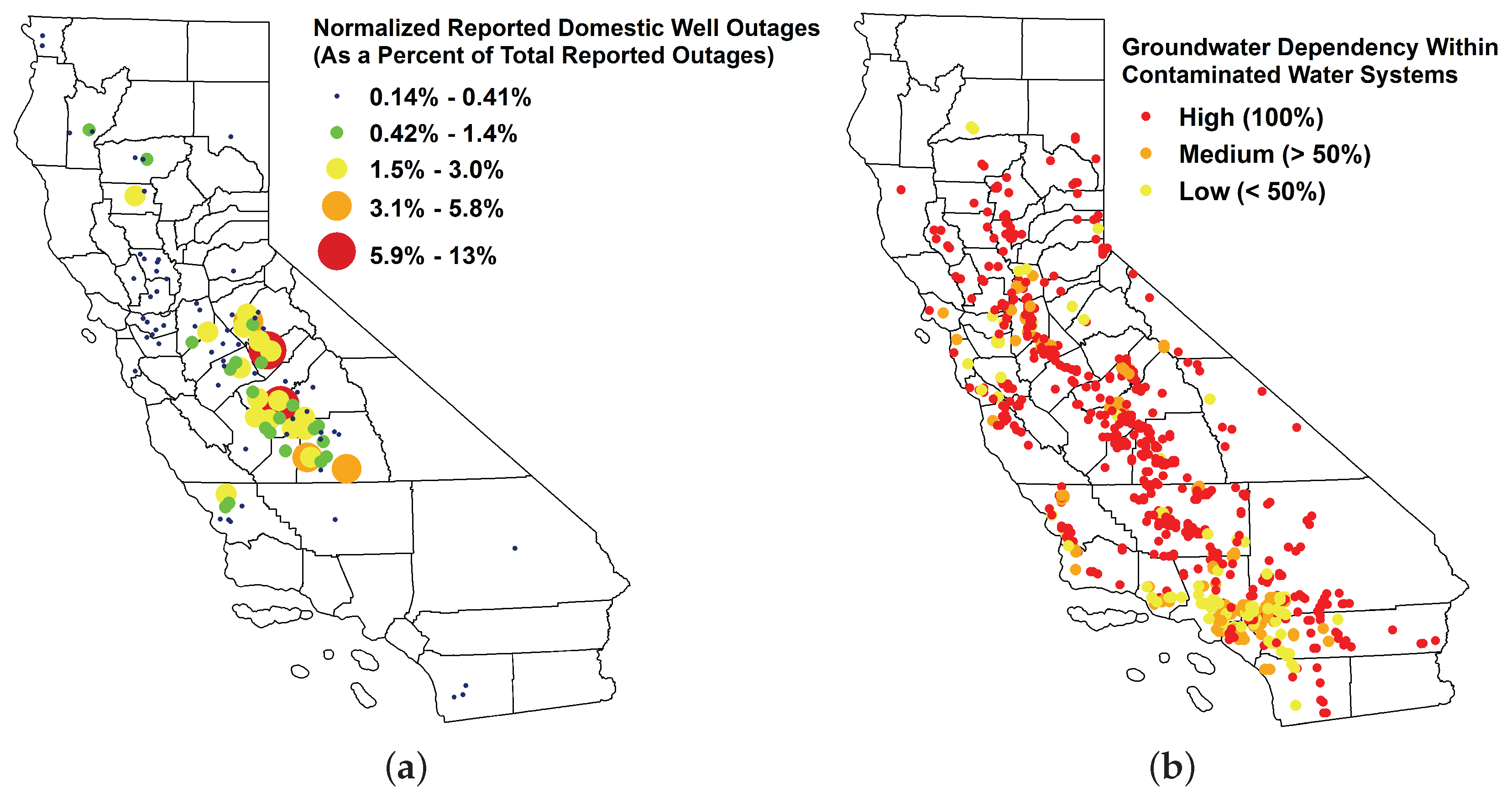
2.1. Domestic Water Shortage Data

A metric was developed to identify areas in California vulnerable to domestic water shortages and/or contamination. Household well shortage data compiled by the California Office of Planning and Research (OPR) were analyzed to understand the geospatial distribution of domestic water shortages reported across the state [7]. The number of household water shortages were normalized to derive a fractional distribution of shortage risk by dividing the number of reported shortages in each town/city by the total number of shortages reported across the state. The normalized values were assigned a weighted distribution such that the locations with the fewest and highest number of reported shortages were assigned values of 50 and 100, respectively.

A map of the normalized water outages, as reported for the Office of Planning and Research, with larger circles representing a greater percentage of well reports in each urban center, is included in Figure 1a. The city with the highest number of well outage reports was Fresno, followed by a series of other towns in or adjacent to the Central Valley.

A second dataset published by the California SWRCB lists all known contaminated wells within public water systems in 2010, as well as each water system’s level of groundwater dependency [8]. Unique well IDs from the report were merged with geospatial coordinates from the SWRCB’s Groundwater Ambient Monitoring and Assessment (GAMA) program to compile a geospatial database of each contaminated well and its community system’s level of groundwater dependency [25]. Weights of 10, 30 and 50 were assigned to contaminated wells occurring in systems with groundwater dependencies of less than 50%, greater than 50%, and 100%, respectively [8]. Wells with an undetermined level of groundwater dependency were removed. A geospatial representation of the contaminated water systems in California is shown in Figure 1b. The colors reflect the level of groundwater dependecy for each system, with yellow representing below 50% dependency, orange representing above 50% dependency, and red representing 100% dependency. Many of the red points are located in the Central Valley, similar to the results shown on the map of normalized domestic well outages.

The summed weighted values, reflecting both water shortage incidents and contaminated wells, were plotted in ArcGIS (10.2.2, ESRI, Redlands, CA, USA) and interpolated using Inverse Distance Weighting (IDW), revealing a spatially resolved estimation of domestic water shortage risk, shown in red in Figure 2. It can be seen that the locations with the greatest vulnerability to domestic water shortages are mainly in the Central Valley. Areas farther south, such as Los Angeles, have more water security since they receive water from multiple sources, in addition to groundwater. Although some parts of California, particularly the urban parts of Southern California, receive water from aqueducts such as the Colorado River Aqueduct, the Los Angeles Aqueduct (in the territory of the Los Angeles Department of Water and Power), and the California State Water Project, these supply options are geospatially limited in terms of the service areas to which they provide water [26].

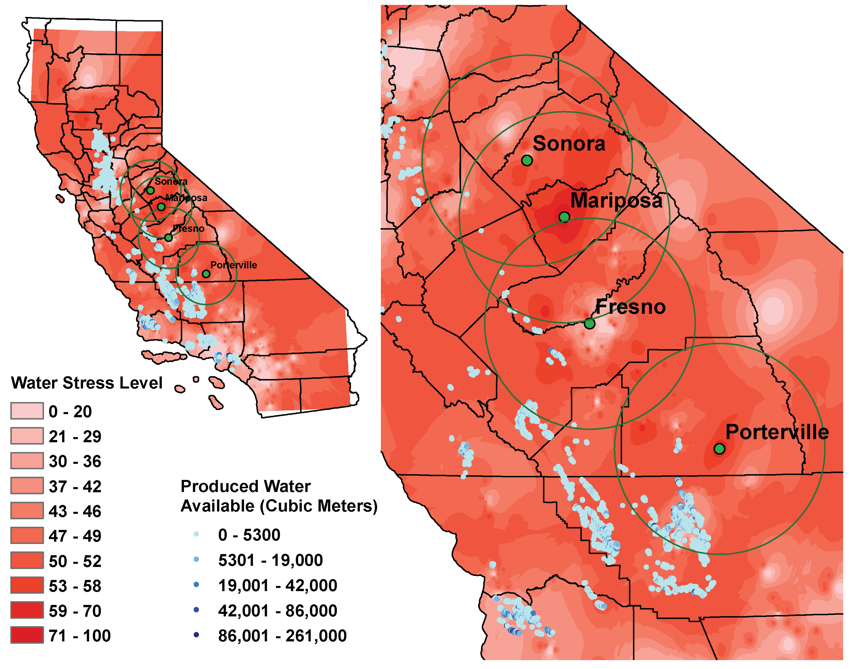
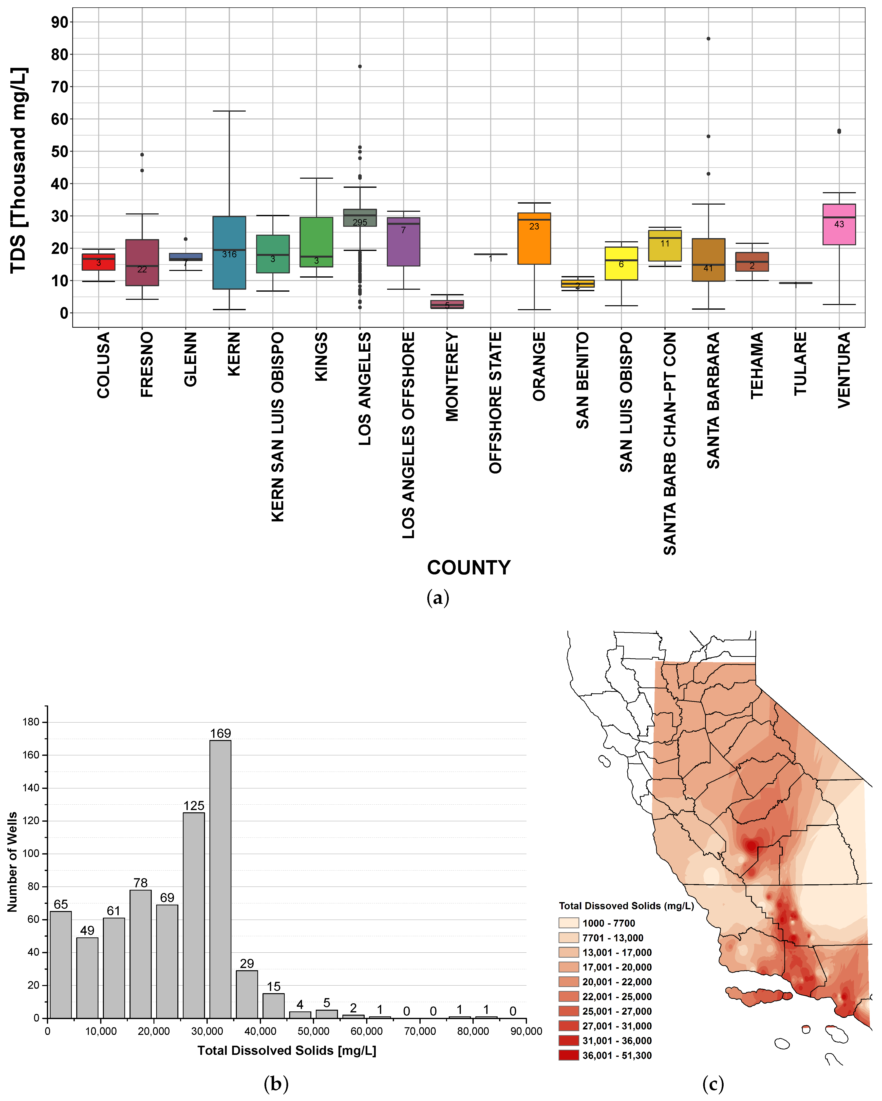
2.2. Oil and Gas Production Produced Water Data

Publicly available datasets from the US Geological Survey (USGS) and the California Department of Oil, Gas and Geothermal Resources (DOGGR) were used to identify the location, volume, and quality of produced water at the site of oil and natural gas production across the state [27,28]. The USGS Produced Waters Geochemical Database contains the location and physical and chemical geochemical properties of 161,915 produced water samples across the conterminous United States, of which 7430 samples were located in California and used in the analysis [27]. Sampling time intervals among individual wells were not uniform since sampling data are compiled from different sources, so the most recently sampled data were analyzed for each well (i.e., the Produced Waters Geochemical Database used was version 2.1, released on October 2015). DOGGR produced water data provided comprehensive monthly volumetric data with well ID number, well type, status and production of non-confidential wells across California [28].

Challenges arose when trying to merge produced water databases since well identification numbers used in the USGS and DOGGR water quality and water quantity databases are not consistent. Furthermore, the number of available USGS well data records was much lower than available DOGGR records. Thus, the produced water quality of wells was estimated using IDW interpolation based on the total dissolved solids (TDS), assuming that produced water quality within a localized region is similar. After interpolation, produced water quality values were extracted onto a map populated with DOGGR’s volumetric produced water data, coupling produced water quantity and quality data for each well. Figure 3c contains the interpolations of the TDS levels of produced water in California. Since the IDW function only interpolates where well data were available, the interpolation did not span across the entirety of California, as USGS’ data did not include wells into the northernmost and southeastern regions of California. Since most water stress occurs in Central California, these omissions did not significantly impact the analysis.

The quality of produced water ranges from nearly the same TDS as freshwater to an order of magnitude more TDS than seawater [27,29]. The box plot in Figure 3a and histogram in Figure 3b provide information on the range of TDS levels at California oil and gas wells. Since the energy-intensity of treating water varies inversely with TDS, initial quality typically dictates the economic feasibility of treating produced water [30]. Reverse Osmosis (RO) desalination typically consumes electrical energy at a rate of 3–4 kWh/m${}^3$, primarily to drive water through a membrane to remove contaminants [31]. Desalinating lower-salinity brackish water costs less economically and energetically, with energy consumption values of 0.5–2.5 kWh/m${}^3$ due to lower TDS levels (5000–25,000 mg/L) [31,32]. For this analysis, an upper TDS limit of 25,000 mg/L was selected as a conservative upper-threshold for selecting source water viable for treatment.

All wells with produced water under this threshold were filtered into a geospatial dataset to be analyzed and are illustrated on the interpolated water stress metric map in Figure 2. Along with TDS levels, there are concerns over other materials in produced water, such as production chemicals and naturally occurring radioactive materials (NORM) [17,33]. However, NORM levels in California have been found to be relatively low [34,35].

2.3. Techno-Economic Analysis

Reverse osmosis (RO) has been successfully utilized for treating water produced during oil and gas operations. Pre-treatment is necessary for preserving the integrity of the RO membrane. Usually, such pre-treatment is achieved by some types of filtration, such as coal, sand, and, more recently, microfiltration [33,36,37]. De-oiling water prior to the RO process is the most important pretreatment step when considering produced water [36,38]. Currently, the vast majority (over 99%) of produced water is already de-oiled on-site in California [39]. Pre-treatment, including removal of oil and suspended matter, is generally necessary prior to injection in a Class II well to prevent plugging in the receiving formation, which can cause pressure build-up and damage to the injection pumps [40]. Thus, the incremental cost for RO pre-treatment, compared to business-as-usual pre-treatment of produced water prior to Class II well injection, is likely negligible. Although higher salinity water can be treated with thermal desalination technologies, these processes are generally energy and capital intensive [41]. Other emerging technologies may be promising in terms of energy efficiency but are not yet available at commercial scale [16].

The total annual cost of the RO treatment system, C${}_T$, reflects annualized construction, C${}_I$, and operational, C${}_O$, costs:

$$C_T=C_I+C_O,$$

(1)

$$C_I=P_I\times [\frac{{(i+1)}^t}{{(i+1)}^t-1}]\times Q,$$

(2)

$$C_O=P_O\times [\frac{i{(i+1)}^t}{{(i+1)}^t-1}]\times Q,$$

(3)

where P${}_I$ is the present value of the initial capital cost per unit volume of treated water, i is the annual interest rate, t is the amortization period, P${}_O$ is the operational cost per unit volume of treated water, and Q is the annual amount of recovered water after treatment.

The energy needed to pump water from its source to end-use, E, is dependent on the change in elevation from the source to the destination and frictional losses across the piping network, as shown in Equation (4):

$$E=\rho Qg\Delta h,$$

(4)

where ρ is the density of water, g is the acceleration due to gravity, and Q is the volume of recovered water after treatment defined in

Table 1. Available quantities of produced water less than 25,000 mg/L total dissolved solids before and after reverse osmosis (RO) treatment at varying distances from Fresno, Mariposa, Sonora, and Porterville, assuming a 50% RO recovery rate. Pumping, treatment (including annualized capital and operational) and disposal costs of moving and preparing water for targeted demand centers based on treatable volumes.

	Radius	Produced Water Available (1000 m${}^{\mathbf{3}}$)					Water After Treatment (1000 m${}^{\mathbf{3}}$)					Water After Treatment (People-Years)
	(miles/km)	Fresno	Mariposa	Sonora	Porterville		Fresno	Mariposa	Sonora	Porterville		Fresno	Mariposa	Sonora	Porterville
Volumes	15/24	–	–	–	–		–	–	–	–		–	–	–	–
	30/48	610	–	–	3800		310	–	–	1900		3000	–	–	18,000
	50/80	950	0.0042	0.0042	72,000		450	0.0020	0.0022	37,000		4500	0.019	0.021	350,000
	75/121	8700	610	18	120,000		4200	310	8.7	64,000		41,000	3000	85	600,000
	100/161	79,000	7200	640	140,000		38,000	3600	330	68,000		380,000	35,000	3100	650,000
	Radius	Pumping Cost of Treated Water (1000 USD)					Annualized RO Treatment Costs (1000 USD)					Brine Disposal Costs (1000 USD)
	(miles/km)	Fresno	Mariposa	Sonora	Porterville		Fresno	Mariposa	Sonora	Porterville		Fresno	Mariposa	Sonora	Porterville
Costs	15/24	–	–	–	–		–	–	–	–		–	–	–	–
	30/48	0.95–1.3	–	–	30–40		58	–	–	350		5.2	–	–	32
	50/80	1.5–2.0	0.00029–0.00038	0.00028–0.00038	600–790		88	0.0004	0.0004	6900		7.6	0.000033	0.000036	620
	75/121	15–19	45–60	1.2–1.5	1000–1100		810	58	1.7	12,000		70	5.2	0.15	1800
	100/161	140–180	520–700	43–57	1100–1500		7300	670	61	13,000		630	60	5.5	1100

. Total head loss, $\Delta h$, is defined as the sum of head losses due to elevation, $h_e$, and pipe friction losses, $h_f$:

$$\Delta h=h_e+h_f.$$

(5)

Elevation gains between the location of oil and gas activities and each demand center target were calculated from the USGS’ National Map Elevation database [42]. Frictional losses were calculated in Equation (6):

$$h_f=f{\displaystyle \frac{v^2}{2g}}{\displaystyle \frac{\Delta L}{d}},$$

(6)

where f is the friction factor, v is the flow velocity of water through the pipes, $\Delta L$ represents the radial distance from water source to city, and d is the diameter of the pipe. The values for f, v, and d, used in this study reflect values used by Stillwell et al. [43].

The cost to transport water was determined using electricity cost data provided from the U.S. Energy Information Administration (EIA) [44]. The costs to pump various quantities of produced water to demand centers are shown in Table 1 and assume that only half of the available produced water would be recovered and moved after treatment. The lower and upper cost bounds reflect industrial and commercial electricity rates, respectively.

The cost of brine disposal via Class II injection is influenced by pipeline transport and/or trucking costs, but these costs are not regulated or recorded, and thus generally not publicly available [45] . Disposal costs in Table 1 reflect a Class II injection disposal cost of $16.80/m${}^3$ [45].

3. Results

Although California’s oil and gas operations and existing water shortages are largely concentrated in the Central Valley, moving water to demand centers would still require relatively long pipeline networks [20]. The cost of building out piping infrastructure is not included in this analysis but would be a substantial upfront cost. The volumes of produced water available within several radii of domestic water shortage hotspots before and after desalination are shown in Table 1. People-years of potable water that could be served by produced water within each radius reflect an average Californian domestic water use rate of 290 liters per day and an RO recovery rate of 50% (since a large fraction of water is rejected as brine) [46,47]. While there are not significant quantities of produced water that can be treated within 15 miles of target cities, more produced water becomes available as the radius of interest around these cities is extended. Moving water to Mariposa and Sonora was more expensive than the other locations because these cities are at elevations of over 1000 feet above sea level. While the cost to pump the water to Fresno was cheapest, Porterville provided greater volumes of potential water generation due to its proximity to oil and gas activities. Within a 100-mile radius, Porterville has access to over 132 million m${}^3$ of treatable produced water, which equates to approximately 650,000 people-years worth of water post-treatment. Porterville, despite its water stress, was the fastest-growing city in California in 2015, so identifying long-term solutions for its water-stressed population is particularly timely [48].

While our model considers an upward threshold of 25,000 mg/L, if this threshold was increased to 35,000 mg/L, which is comparable to the Pacific Ocean, another 130 million m${}^3$ in the state would become available for treatment. However, across the four cities that we analyzed, the additional quantities available within a 50 mile radius would not be significant (Fresno: 270,925 m${}^3$, Mariposa: 0 m${}^3$, Sonora: 0 m${}^3$, Porterville: 0 m${}^3$), and the costs of desalinating water would increase.

The annual volume of available produced water aggregated for all four cities is estimated as nearly 230 million m${}^3$ when considered across 100-mile radi from each location. The unit economic and energy costs of RO depend heavily on the treatment plant scale, with the unit cost of treating water with RO decreasing with increasing capacity. Thus, P${}_I$ ($1.57/m${}^3$) and P${}_O$ ($1.15/m${}^3$) values were selected based on an RO system of similar scale in Turkey that treats 100 m${}^3$/day of produced water from 40 oil and gas wells [49]. For reference, a large-scale (>20,000 m${}^3$/day) modern brackish water desalination plant can operate at a cost as low as $0.31/m${}^3$ [50]. Total annual cost assumes an operational lifetime of 30 years and a current interest rate (0.5% year${}^{-1}$) [51]. The $1.15/m${}^3$ operational cost includes energy costs, daily maintenance costs and chemical costs. Membranes of RO systems are usually replaced up to every 10 years, with specific membrane replacement costs ranging from $0.04/m${}^3$ to $0.36/m${}^3$ [52]. A membrane cost of $0.15/m${}^3$ was used in this analysis based on a similar scale seawater desalination plant in Oia, Greece [53]. Collectively, the P${}_O$ utilized in this analysis was $1.3/m${}^3$. On average, membrane costs represent a very small fraction of the total treatment cost. Results are summarized in Table 1.

This analysis evaluated the costs of producing and moving potable water from an RO treatment plant to large residential and commercial demand centers to provide an upper threshold for energetic and economic costs. However, utilizing treated water for non-potable uses might be a more politically and socially feasible strategy for upgrading this water and would result in higher product volumes as ultra-pure water from the RO plant could be blended with larger volumes of lower quality water sources. The economics of whether or not produced water becomes an economically feasible water source, whether for nearby agricultural applications or for more distant industrial, commercial or residential uses, depends on the cost of competing water supplies. Wholesale costs averaged $0.20/m${}^3$, $0.39/m${}^3$, $0.37/m${}^3$, and $0.22/m${}^3$ in Fresno, Mariposa, Sonara and Porterville, respectively, for 50 to 100 mile distances. The wholesale unit cost of delivered treated water was largely driven by treatment, rather than pumping. While these estimates would shift according to actual water treatment, pumping, and brine disposal configurations, as well as piping installation, permission, and other region-specific costs, these estimates offer a general order of magnitude estimate of wholesale costs to compare against other water supplies (see

Table 2. The wholesale costs of treating and pumping potable water from various distances from targeted urban centers, as compared with agricultural, public supply and bottle water retail prices in the Central Valley area.

Radius (Miles/km)	Fresno per m${}^{\mathbf{3}}$	Mariposa per m${}^{\mathbf{3}}$	Sonora per m${}^{\mathbf{3}}$	Porterville per m${}^{\mathbf{3}}$
15/24	–	–	–	–
30/48	$0.19	–	–	$0.21
50/80	$0.19	$0.38	$0.36	$0.21
75/121	$0.19	$0.38	$0.36	$0.21
100/161	$0.19	$0.38	$0.36	$0.21
Agricultural Water (Retail)	$0.014 [54] to $0.89 [55] per m${}^3$
California Public Water Supply (Retail)	$0.31 [56] (Porterville) to $0.45 [57] (Fresno) per m${}^3$
Bottled Water (Retail)	$320.00 [58] per m${}^3$

).

Agricultural water is typically cheap and used in very large quantities, so the cost and scale of water needs might be mismatched with the proposed strategy. The retail price of agricultural water in California varies significantly by water district, but prices in parts of Merced and Fresno County ranged anywhere from $0.014 to $0.89/m${}^3$ in recent years [54,55]. Blending treated water with other degraded water sources can boost useable water supplies and make water more cost competitive with other agricultural water sources.

While competitiveness with current retail drinking water supplies would depend on piping infrastructure costs and retail markup, the costs of the proposed pumping and treatment systems are very favorable to bottled water, which is currently being exploited as a solution to outages in many areas of the state. In comparison, the price of bottled water sold in the US averaged $320.00/m${}^3$ in 2014, which is several orders of magnitude higher than the cost of treatment and transportation of produced water [58,59]. However, current policy and social barriers would likely restrict using treated produced water as a potable water source in the near term.

4. Discussion

One major barrier to RO implementation includes the cost of electricity consumption, representing up to 50% of the total cost of producing water with RO [60]. However, California is approaching a unique conundrum when it comes to electricity production. In 2015, California passed Senate Bill 350, which increased its renewable portfolio standard from 33% to 50% by 2030, which is anticipated to result in 12,000 GWh electricity overgeneration per year, mainly due to the excess of solar capacity during daytime hours [7,61]. This solar growth is expected to significantly decrease the wholesale electricity prices during daytime hours, pointing to an opportunity to incorporate flexible loads that can be timed according to solar availability. Thus, ramping up treatment capacity during the day to use excess solar generation could significantly decrease costs and relieve potential overgeneration. While electric power intermittency has been shown to accelerate membrane degradation due to pressure and flow rate fluctuations [62,63], incorporating mechanical pressure stabilizers or storage into integrated photovoltaics or wind-powered desalination facilities can boost performance by maintaining a constant permeate flowrate [60,62,63].

A second common barrier to inland RO is the difficulty of ultimate brine discharge [45]. The transport of brine concentrate from inland RO plants is often cost prohibitive, reducing the economic feasibility of such facilities [41]. However, California’s regions of produced water generation are co-located with thousands of Class II injection wells, which could be utilized to inject brine concentrate, since these wells are already permitted for produced water discharges and infrastructure is already in place. In 2015, 80% (369 million m${}^3$) of the total produced water (468 million m${}^3$) was injected into Class II wells as the final disposal method in California [64,65,66,67]. The result of this study indicated that 115 million m${}^3$ of brine would require a disposal, which is within the current holding capability of Class II wells. This is a unique opportunity for inland brackish water desalination that is not available in many regions of the US due to geological constraints.

5. Conclusions

To conclude, the cost of treating and transporting produced water to cities for beneficial use is dependent upon the quality and quantity of source water, as well as the distance, elevation, and desired end quality of the water. While the total cost of upgrading degraded water sources can be quite high, growing water scarcity places a new precedent on utilizing alternative water sources. Although other alternative sources of water exist, over half a billion cubic meters of produced water from oil and gas operations in California are being produced each year, and these supplies are generally co-located with regions already experiencing devastating water shortages. Locating such a water management strategy in California’s Central Valley offers a number of synergistic opportunities for utilizing produced water for beneficial uses to offset the cost of desalination, while addressing critical water shortages issues in adjacent communities. Given the state’s ongoing drought in conjunction with the prospect of cheap, daytime solar electricity and widely available Class II injection well sites for brine, inland brackish water desalination might become an attractive option for utilizing degraded water sources such as produced water from oil and gas extraction for beneficial uses, especially as the cost of baseline water supplies increase.

References

1. Faunt, C.C.; Sneed, M.; Traum, J.; Brandt, J.T. Water availability and land subsidence in the Central Valley, California, USA. Hydrogeol J. 2015, 24, 675–684. [Google Scholar] [CrossRef]
2. Griffin, D.; Anchukaitis, K.J. How unusual is the 2012–2014 California drought? Geophys. Res. Lett. 2014, 41, 9017–9023. [Google Scholar] [CrossRef]
3. Fuchs, B. U.S. Drought Monitor—California; National Drought Mitigation Center: Lincoln, NE, USA, 2016. [Google Scholar]
4. Steinschneider, S.; Lall, U. El Nino and the U.S. precipitation and floods: What was expected for the January–March 2016 winter hydroclimate that is now unfolding? Water Resour. Res. 2016, 52, 1498–1501. [Google Scholar] [CrossRef]
5. Famiglietti, J.S.; Lo, M.; Ho, S.L.; Bethune, J.; Anderson, K.J.; Syed, T.H.; Swenson, S.C.; De Linage, C.R.; Rodell, M. Satellites measure recent rates of groundwater depletion in California’s Central Valley. Geophys. Res. Lett. 2011, 38, 2–5. [Google Scholar] [CrossRef]
6. Ritchel, M. California Farmers Dig Deeper for Water, Sipping Their Neighbors Dry; The New York Times: New York, NY, USA, 2015; pp. 1–9. [Google Scholar]
7. Household Water Shortage Intake Form Data; Technical Report; California Office of Planning and Research: Sacramento, CA, USA, 2015.
8. State Water Resources Control Board. Communities that Rely on a Contaminated Groundwater Source for Drinking Water; State Water Resources Control Board: Sacramento, CA, USA, 2013; p. 178.
9. Hanak, E.; Mount, J.; Chappelle, C.; Lund, J.; Medellin-Azuara, J.; Moyle, P.; Seavy, N. What If California’s Drought Continues? Public Policy Institute of California: San Francisco, CA, USA, 2015. [Google Scholar]
10. Cooley, C.; Ajami, N. Key Issues for Seawater Desalination in California Cost and Financing. World’s Water 2014, 8, 93–121. [Google Scholar]
11. Mccool, B.C.; Rahardianto, A.; Faria, J.; Kovac, K.; Lara, D.; Cohen, Y. Feasibility of reverse osmosis desalination of brackish agricultural drainage water in the San Joaquin Valley. Desalination 2010, 261, 240–250. [Google Scholar] [CrossRef]
12. Stein, S.; Russak, A.; Sivan, O.; Yechieli, Y.; Rahav, E.; Oren, Y.; Kasher, R. Saline groundwater from coastal aquifers as a source for desalination. Environ. Sci. Technol. 2016, 50, 1955–1963. [Google Scholar] [CrossRef] [PubMed]
13. Stuber, M.D. Optimal design of fossil-solar hybrid thermal desalination for saline agricultural drainage water reuse. Renew. Energy 2016, 89, 552–563. [Google Scholar] [CrossRef]
14. Clayton, M.E.; Stillwell, A.S.; Webber, M.E. Implementation of brackish groundwater desalination using wind-generated electricity: A case study of the energy-water nexus in Texas. Sustainability 2014, 6, 758–778. [Google Scholar] [CrossRef]
15. Boo, C.; Lee, J.; Elimelech, M. Omniphobic Polyvinylidene Fluoride (PVDF) Membrane for Desalination of Shale Gas Produced Water by Membrane Distillation. Environ. Sci. Technol. 2016, 50, 12275–12282. [Google Scholar] [CrossRef] [PubMed]
16. Shaffer, D.L.; Chavez, L.H.A.; Ben-sasson, M.; Castrillo, S.R.; Yip, N.Y.; Elimelech, M. Desalination and Reuse of High-Salinity Shale Gas Produced Water: Drivers, Technologies, and Future Directions. Environ. Sci. Technol. 2013, 47, 9569–9583. [Google Scholar] [CrossRef] [PubMed]
17. Guerra, K.; Dahm, K.; Dundorf, S. Oil and Gas Produced Water Management and Beneficial Use in the Western United States; Technical Report 157; Bureau of Reclamation: Denver, CO, USA, 2011.
18. Kondash, A.; Vengosh, A. Water Footprint of Hydraulic Fracturing. Environ. Sci. Technol. Lett. 2015, 10, 276–280. [Google Scholar] [CrossRef]
19. Oikonomou, P.D.; Kallenberger, J.A.; Waskom, R.M.; Boone, K.K.; Plombon, E.N.; Ryan, J.N. Water acquisition and use during unconventional oil and gas development and the existing data challenges. J. Environ. Manag. 2016, 181, 36–47. [Google Scholar] [CrossRef] [PubMed]
20. Tiedeman, K.; Yeh, S.; Scanlon, B.; Teter, J.; Mishra, G.S. Recent Trends in Water Use and Production for California Conventional and Unconventional Oil Production. Environ. Sci. Technol. 2016, 50, 7904–7912. [Google Scholar] [CrossRef] [PubMed]
21. Murray, K.E. State-scale perspective on water use and production associated with oil and gas operations, Oklahoma, U.S. Environ. Sci. Technol. 2013, 47, 4918–4925. [Google Scholar] [CrossRef] [PubMed]
22. 2014 Preliminary Report of California Oil and Gas Production Statistics; Technical Report; Division of Oil, Gas, and Geothermal Resources: Sacramento, CA, USA, 2015.
23. Kuwayama, Y.; Olmstead, S.; Krupnick, A. Water Quality and Quantity Impacts of Hydraulic Fracturing. Curr. Sustain. Renew. Energy Rep. 2015, 2, 17–24. [Google Scholar] [CrossRef]
24. Shonkoff, S.B.C.; Stringfellow, W.T.; Domen, J.K. Preliminary Hazard Assessment of Chemical Additives Used in Oil and Gas Fields that Reuse Their Produced Water for Agricultural Irrigation in The San Joaquin Valley of California; Technical Report; PSE Healthy Energy, Inc.: Oakland, CA, USA, 2016. [Google Scholar]
25. State Water Resources Control Board. GAMA—Groundwater Ambient Monitoring and Assessment Program; State Water Resources Control Board: Sacramento, CA, USA, 2015.
26. Sanders, K.T. The energy trade-offs of adapting to a water-scarce future: Case study of Los Angeles. Int. J. Water Resour. Dev. 2016, 32, 362–378. [Google Scholar] [CrossRef]
27. Blondes, M.S.; Gans, K.D.; Thorsden, J.J.; Reidy, M.E.; Thomas, B.; Engle, M.A.; Kharaka, Y.K.; Rowan, E.L. U.S. Geological Survey National Produced Waters Geochemical Database v2.1 (PROVISIONAL). 2015. Available online: http://xxx.lanl.gov/abs/arXiv:1011.1669v3 (accessed on 12 November 2015). [Google Scholar]
28. Monthly Production and Injection Databases; Technical Report; Division of Oil, Gas, and Geothermal Resources: Sacramento, CA, USA, 2016.
29. Glazer, Y.R.; Kjellsson, J.B.; Sanders, K.T.; Webber, M.E. Potential for Using Energy from Flared Gas for On-Site Hydraulic Fracturing Wastewater Treatment in Texas. Environ. Sci. Technol. Lett. 2014, 1, 300–304. [Google Scholar] [CrossRef]
30. Sanders, K.T.; Webber, M.E. Evaluating the energy consumed for water use in the United States. Environ. Res. Lett. 2012. [Google Scholar] [CrossRef]
31. Ghaffour, N.; Missimer, T.M.; Amy, G.L. Technical review and evaluation of the economics of water desalination: Current and future challenges for better water supply sustainability. Desalination 2013, 309, 197–207. [Google Scholar] [CrossRef]
32. Elimelech, M.; Phillip, W.A. The Future of Seawater and the Environment: Energy, Technology, and the Environment. Science 2011, 333, 712–718. [Google Scholar] [CrossRef] [PubMed]
33. Fakhru’l-Razi, A.; Pendashteh, A.; Abdullah, L.C.; Biak, D.R.A.; Madaeni, S.S.; Abidin, Z.Z. Review of technologies for oil and gas produced water treatment. J. Hazard. Mater. 2009, 170, 530–551. [Google Scholar] [CrossRef] [PubMed]
34. A Study of NORM Associated with Oil and Gas Production Operations in California; Technical Report; Department of Health Services Radiologic Health Branch and Division of Oil, Gas, and Geothermal Resources: Sacramento, CA, USA, 1996.
35. U.S. Environmental Protection Agency. TENORM: Oil and Gas Production Wastes; U.S. Environmental Protection Agency: Washington, DC, USA. Available online: https://www.epa.gov/radiation/tenorm-oil-and-gas-production-wastes (accessed on 29 October 2016).
36. Kim, Y.M.; Kim, S.J.; Kim, Y.S.; Lee, S.; Kim, I.S.; Kim, J.H. Overview of systems engineering approaches for a large-scale seawater desalination plant with a reverse osmosis network. Desalination 2009, 238, 312–332. [Google Scholar] [CrossRef]
37. Voutchkov, N. Considerations for selection of seawater filtration pretreatment system. Desalination 2010, 261, 354–364. [Google Scholar] [CrossRef]
38. Arthur, J.D.; Langhus, B.G.; Patel, C. Technical Summary of Oil & Gas Produced Water Treatment Technologies; Technical Report; ALL Consulting: Tulsa, OK, USA, 2005. [Google Scholar]
39. Water Report Summary Division of Oil, Gas, and Geothermal Resources Second Quarter 2015; Technical Report; Division of Oil, Gas, and Geothermal Resources: Sacramento, CA, USA, 2015.
40. Wiedeman, A. Regulation of Produced Water By the U.S. Environmental Protection Agency. In Produced Water 2: Environmental Issues and Mitigation Technologies; Springer: New York, NY, USA, 1996; pp. 27–41. [Google Scholar]
41. Greenlee, L.F.; Lawler, D.F.; Freeman, B.D.; Marrot, B.; Moulin, P. Reverse osmosis desalination: Water sources, technology, and today’s challenges. Water Res. 2009, 43, 2317–2348. [Google Scholar] [CrossRef] [PubMed]
42. U.S. Geological Survey. The National Map Elevation; U.S. Geological Survey: Reston, VA, USA, 2015.
43. Stillwell, A.S.; King, C.W.; Webber, M.E. Desalination and Long-Haul Water Transfer as a Water Supply for Dallas, Texas: A Case Study of the Energy-Water Nexus in Texas. Texas Water J. 2010, 1, 33–41. [Google Scholar]
44. U.S. Energy Information Adminstration. Electric Power Monthly with Data for March 2016; Technical Report; U.S. Energy Information Adminstration: Washington, DC, USA, 2016.
45. Sullivan, E.J.; Chu, S.; Stauffer, P.H.; Middleton, R.S.; Pawar, R.J. A method and cost model for treatment of water extracted during geologic CO2 storage. Int. J. Greenh. Gas Control 2013, 12, 372–381. [Google Scholar] [CrossRef]
46. California Environmental Protection Agency. November 2015 Water Conservation Report by Supplier; Technical Report; California Environmental Protection Agency: Sacramento, CA, USA, 2015.
47. Mezher, T.; Fath, H.; Abbas, Z.; Khaled, A. Techno-economic assessment and environmental impacts of desalination technologies. Desalination 2011, 266, 263–273. [Google Scholar] [CrossRef]
48. Benjamin, M. Porterville, Clovis Lead Central San Joaquin Valley in Population Growth in 2015; The Fresno Bee: Fresno, CA, USA, 2016. [Google Scholar]
49. Çakmakce, M.; Kayaalp, N.; Koyuncu, I. Desalination of produced water from oil production fields by membrane processes. Desalination 2008, 222, 176–186. [Google Scholar] [CrossRef]
50. Sauvet-Goichon, B. Ashkelon desalination plant—A successful challenge. Desalination 2007, 203, 75–81. [Google Scholar] [CrossRef]
51. Board of Governors of the Federal Reserve System. Selected Interest Rates (Daily). 2016. Available online: https://www.federalreserve.gov/releases/h15/ (accessed on 29 October 2016). [Google Scholar]
52. Avlonitis, S.A.; Kouroumbas, K.; Vlachakis, N. Energy consumption and membrane replacement cost for seawater RO desalination plants. Desalination 2003, 157, 151–158. [Google Scholar] [CrossRef]
53. Avlonitis, S.A. Operational water cost and productivity improvements for small-size RO desalination plants. Desalination 2002, 142, 295–304. [Google Scholar] [CrossRef]
54. Baldocchi, D. California Drought: Charge True Cost of Agricultural Water; San Francisco Chronicle: San Francisco, CA, USA, 2015. [Google Scholar]
55. Vekshin, A. California Water Prices Soar for Farmers as Drought Grows; Bloomberg: New York, NY, USA, 2014. [Google Scholar]
56. City of Porterville. Utility Rates & Information; City of Porterville: Porterville, CA, USA, 2015. [Google Scholar]
57. Municipal Financial Services. Water Utility Financial Plan and Rates Study; Technical Report; Municipal Financial Services: Fresno, CA, USA, 2015. [Google Scholar]
58. International Bottled Water Association. How Much Does Bottled Water Cost? International Bottled Water Association: Alexandria, VA, USA, 2015. [Google Scholar]
59. Nestlé Waters North America Inc. ReadyFresh; Nestlé Waters North America Inc.: Stamford, CT, USA, 2016. [Google Scholar]
60. Gude, V.G. Energy storage for desalination processes powered by renewable energy and waste heat sources. Appl. Energy 2015, 137, 877–898. [Google Scholar] [CrossRef]
61. Investigating a Higher Renewables Portfolio Standard in California; Technical Report; Energy and Environmental Economics, Inc.: San Francisco, CA, USA, 2014.
62. Richards, B.S.; Capão, D.P.S.; Früh, W.G.; Schäfer, A.I. Renewable energy powered membrane technology: Impact of solar irradiance fluctuations on performance of a brackish water reverse osmosis system. Sep. Purif. Technol. 2015, 156, 379–390. [Google Scholar] [CrossRef]
63. Lai, W.; Ma, Q.; Lu, H.; Weng, S.; Fan, J.; Fang, H. Effects of wind intermittence and fluctuation on reverse osmosis desalination process and solution strategies. Desalination 2016, 395, 17–27. [Google Scholar] [CrossRef]
64. SB 1281 Water Report Summary—First Quarter 2015; Technical Report; Division of Oil, Gas, and Geothermal Resources: Sacramento, CA, USA, 2015.
65. SB 1281 Water Report Summary—Second Quarter 2015; Technical Report; Division of Oil, Gas, and Geothermal Resources: Sacramento, CA, USA, 2015.
66. SB 1281 Water Report Summary—Third Quarter 2015; Technical Report; Division of Oil, Gas, and Geothermal Resources: Sacramento, CA, USA, 2016.
67. SB 1281 Water Report Summary—Fourth Quarter 2015; Technical Report; Division of Oil, Gas, and Geothermal Resources: Sacramento, CA, USA, 2016.
Figure 1. (a) Normalized reported domestic groundwater well outages, with larger circles representing a higher percentage of outages [7]; (b) contaminated wells with colored gradient representing dependency of each contaminated well’s water system on groundwater, where yellow is <50% groundwater (GW) dependency, orange is >50% GW dependency, and red is 100% GW dependency [8].
Sustainability 08 01318 g001
Figure 2. A domestic water shortage risk metric was created to identify communities most vulnerable to water supply disruptions. Dark red shading indicates regions most vulnerable to shortages. Produced water volumes with total dissolved solids less than 25,000 mg/L are shown in blue. Fresno, Mariposa, Sonoma, and Porterville had the greatest number of reported domestic well outages in the state. An 80 km (50 mile) radius placed around each city illustrates available produced water feasible for treatment within that distance.
Sustainability 08 01318 g002
Figure 3. (a) Boxplot of produced water in Californian counties by total dissolved solids (TDS) levels [27]. The number on each box plot indicates the number of wells containing produced water quality data in the specified county. The range of TDS varies greatly across counties, and a very large portion of wells have a TDS value that is below the seawater TDS level (approximately 35,000 mg/L); (b) histogram of the TDS levels of produced water in California [27]. Each bin represents the TDS level (in mg/L), and the plot illustrates the number of wells in the state that fall within each TDS range; (c) interpolated values of TDS in California, using data from the United States Geological Survey National Produced Waters Geochemical Database [27]. Darker colors represent higher levels of TDS.
Sustainability 08 01318 g003