Gridded Water Resource Distribution Simulation for China Based on Third-Order Basin Data from 2002

Abstract

Water resources are a key factor for regional sustainable development. However, the published water resource data in China is based on a large geographical scale, such as watershed units, and the data cannot reflect subtle differences in water resource distribution. The paper aimed to distribute water resources of the third-order basin of China into grid-cells of 1 km × 1 km. First, we used Moran’s I index to analyze the spatial pattern of water resources of the third-order basin. Second, we constructed a spatial autocorrelation model between water resources of third-order basins and the associated factors. Third, we applied the model to simulate the gridded water resource distribution and evaluated the simulation accuracy. The results indicated that significant spatial autocorrelation existed among the water resources of third-order basins. Northern China was the low-value clustering area of water resources and Southeast China was the high-value clustering area of water resources. Slope and precipitation were the main factors that influenced the amount of water resources. The simulating accuracy of water resource distribution was very high, apart from some extremely arid regions (Gurbantunggut Desert, Kumtag Desert, and Hexi Desert). On the whole, the gridded water resource distribution map was valid and was helpful for regional water resource management.

1. Introduction

Water resources are a key factor for regional sustainable development. Currently, China is facing increasingly severe water scarcity after experiencing rapid economic development and urbanization [1]. The total water use in China witnessed a sharp increase from 1030 billion m³ in 1950 to 6183 billion m³ in 2013 [2]. The over-exploitation of water resources has led to serious environmental consequences, such as salinity intrusion and ecosystem deterioration [3]. Water shortages have significantly limited the sustainable development of the economy and society in China [4]. Apart from the impact of rapid economic development and urbanization with a large and growing population, poor water resource management and uneven spatial distribution of water resources also contribute significantly to China’s water scarcity [5]. Hence, the quantitative description of water resource distribution is important for water resource management, especially for China with its wide regional disparity of water resources [6]. Currently, the most detailed and comprehensive data of water resources in China, provided by the Minister of Water Resources of China, is derived from the observation of meteorological stations at the scale of third-order basins. The water resource data is the average value calculated based on the polygon statistical units and cannot reveal the actual water resource distribute at the small scale. Moreover, water resource data at a smaller spatial scale is urgently needed in many research fields, such as evaluating water resource constraint intensity on economic growth [2]. Hence, it is necessary to spatially refine the statistical areal water resource data and produce water resource data at a small spatial scale. The objective of this paper is to distribute the water resources of third-order basins of China in 2002 to grid-cells of 1 km × 1 km. To the author’s knowledge, no previous research has been implemented to reveal the distribution of water resources at such a fine scale.

According to the Statistic Bulletin on China Water Activities, regional water resources consist of surface water and groundwater. Surface water is water on the surface of the Earth, such as lakes, rivers, and wetlands. Groundwater is the water present beneath the Earth’s surface in the fractures of rock formations and in soil pore spaces. The surface water can be replenished by recruitment from groundwater and can be lost through seepage into the ground where it becomes groundwater [7]. From the perspective of the water cycle, water enters the atmosphere by the physical process of evapotranspiration, and then water vapor condenses into precipitation under appropriate conditions; part of the precipitation returns to the atmosphere through evapotranspiration and the other enters the ground or remains on the surface [8]. Hence, the amount of regional water resources is influenced by many factors. Precipitation is the main source of regional water resources. Evapotranspiration decreases the amount of regional water resources [9]. Temperature, wind and some other climatic factors bring indirect influence to regional water resources [10]. Some physical geographical factors also have a significant impact on regional water resources [11]. For example, slope and topography influence the convergence of runoff. Land cover affects the runoff infiltration and rainfall interception [12].

Methods of transforming data from one system’s area units to another have a long tradition and have been researched systematically in recent years [13,14]. In practical application, the commonly used methods can be grouped into two categories: areal interpolation methods and statistical modeling methods [15]. Areal interpolation methods transfer the discrete data to continuous data by constructing the quantity relationship between the target zone and source zones according to their spatial relationships (e.g., areal weighting, distance weighting) or some ancillary information (e.g., land use and land cover classes) [16]. This method has been widely applied to generate the surface data of rainfall and temperature [17,18]. The statistical modeling method is based on a functional relationship between dependent variables and independent variables. Take small-area population estimation as an example: population is considered to be highly correlated with urban built-up areas, impervious surfaces, dwelling units, and land use [19]. Hence, researchers used to construct functional relationship models (e.g., ordinary linear regression models, geographically-weighted regression models) between population census data and the associated factors [20].

In this study, we built a statistical model between water resources and the associated factors on the scale of third-order basins and then we applied the model to estimate the water resources of grid-cells (1 km × 1 km). Research results indicated that the simulation accuracy of the gridded water resource distribution was very high. The gridded water resource distribution map shows the subtle differences of water resources and the raster data of the gridded water resource distribution can also be used as an important data source in many research applications, such as the bearing capacity of water resources.

2. Materials and Methods

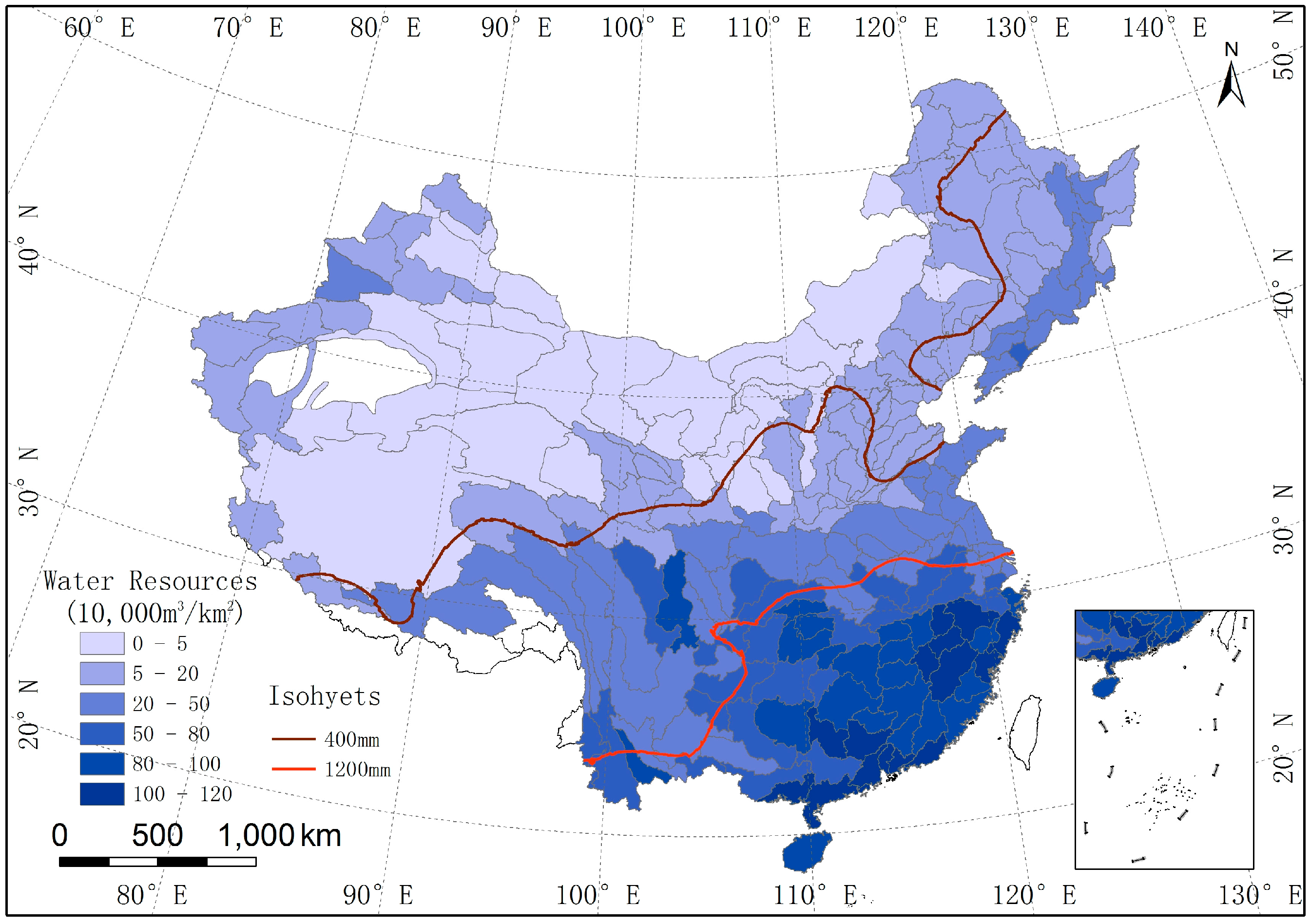
2.1. Study Area and Data

There are 214 third-order basins in China. However, the water resource data of Hong Kong, Taiwan, Macao, and the South China Sea Islands in 2002 are missing and the water resources of Taklimakan Desert were zero. In addition, water resource data of three third-order basins are abnormal. Finally, only 206 third-order basins in China was selected as study areas (Figure 1). Due to the availability and integrity of data, water resource data from 2002 was used for this research. Six different types of raw data were needed: vector boundary data of third-order basins of China, statistical data of water resources of third-order basins of China, daily precipitation/temperature data of meteorological stations, digital elevation model data (DEM), evapotranspiration data, and land cover data. The vector boundary data of third-order basins in China is available for download from the National Geomatics Center of China. Water resource data of third-order basins can be obtained from the 2002 Statistic Bulletin on China Water Activities published by the Ministry of Water Resources of the People’s Republic of China. The daily precipitation/temperature data of meteorological station were obtained from China Meteorological Data Sharing Service System. According to daily precipitation/temperature data, we calculated the annual average precipitation/temperature of every meteorological station and then used the ordinary kriging method to generate 1 km × 1 km grid cell data of precipitation/temperature. The DEM data of China is derived from the shuttle radar topography mission (SRTM) which was implemented by National Aeronautics and Space Administration (NASA) and National Imagery and Mapping Agency (NIMA). We converted the DEM data to the slope data using the surface analysis tool of ArcGIS 10.2 (Environmental Systems Research Institute: Redlands, CA, USA, 2013). Land cover data and evapotranspiration data were obtained from the Institute of Remote Sensing and Digital Earth Chinese Academy of Sciences.

2.2. Study Methods

Due to the first law of geography (everything is related to everything else, but near things are more related than distant things), geospatial data is rarely subjected to independent and identical distribution [21]. Hence, an ordinary linear regression model is inappropriate for geospatial data. We first used global Moran’s I index to verify the spatial autocorrelation of the water resources data of third-order basins of China and analyzed the spatial distribution pattern of water resources based on the local Moran’s I index. Then we constructed a spatial autocorrelation model to simulate the relationship between water resources of third-order basins and the associated factors (precipitation, evapotranspiration, temperature, glacier, forestland, and slope). A spatial autocorrelation model is a standard tool that expands ordinary linear regression model by introducing a spatial weight matrix to quantify the spatial relationship of geographic data [22]. Finally, we applied the empirical model to estimate the water resource amount at a 1 km × 1 km grid scale in China. In addition, we discussed the quality of the spatial autocorrelation model by comparing with an ordinary regression model and conducted the empirical test for the simulation accuracy of water resource distribution by computing the simulation error.

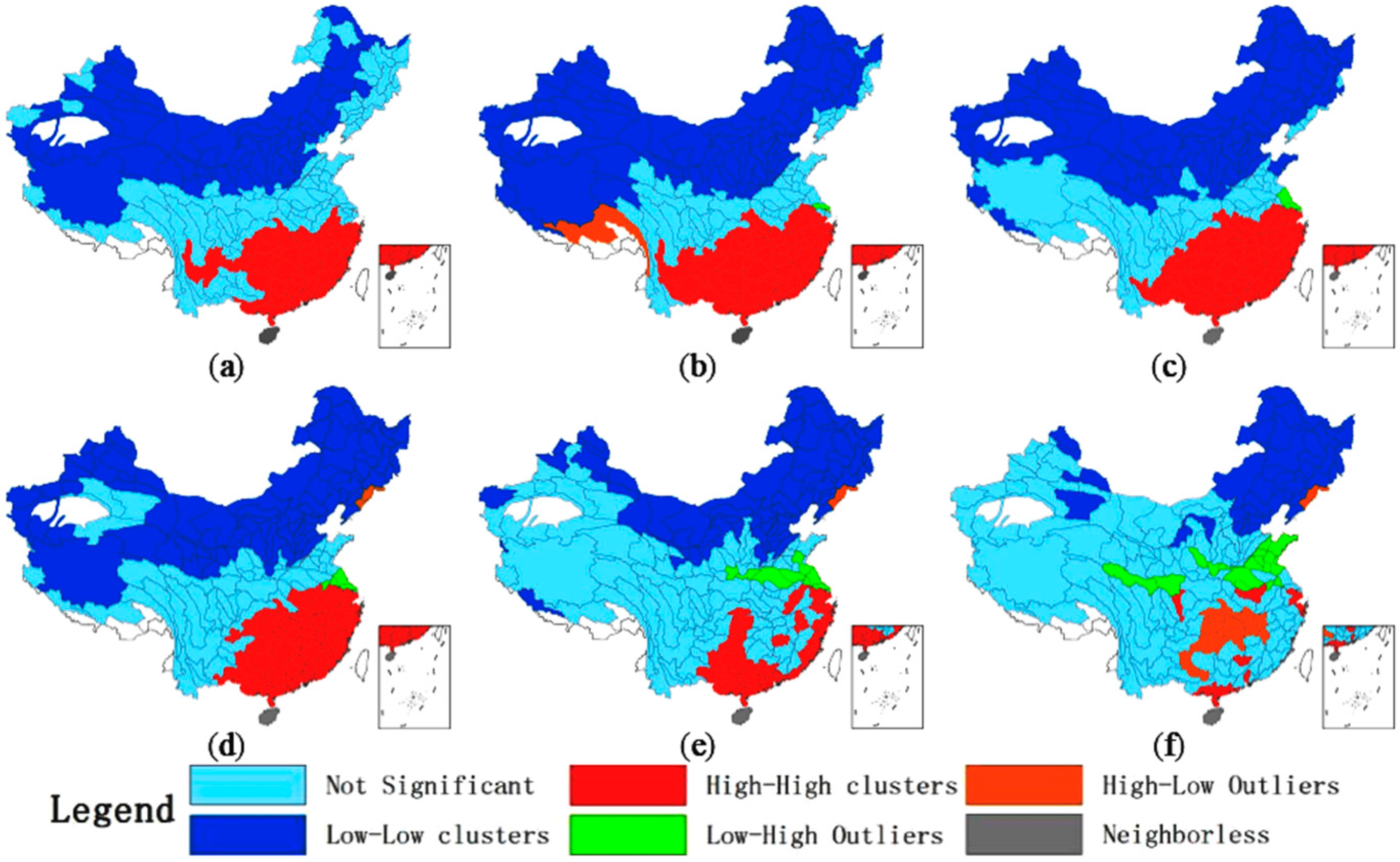
2.2.1. Spatial Autocorrelation Test

This paper used Moran’s I index to test for the spatial autocorrelation of water resources in third-order basins. Moran’s I is of great importance and has been usually used to evaluate the autocorrelation level among the attributive values of the spatial objects in many different research fields [23,24,25]. Moran’s I index includes global Moran’s I and local Moran’s I. Global Moran’s I measures the degree of the spatial autocorrelation as a whole and local Moran’s I quantifies spatial autocorrelation at each location [26]. Their formula can be respectively expressed by Equations (1) and (2):

$$I=\frac{n{\displaystyle \sum _{i=1}^n{\displaystyle \sum _{j=1}^n{w}_{ij}(x_i-\overline{x})(x_j-\overline{x})}}}{({\displaystyle \sum _{i=1}^n{\displaystyle \sum _{j=1}^n{w}_{ij})}}{\displaystyle \sum _{i=1}^n{(x_i-\overline{x})}^2}}$$

(1)

$$I_i=\frac{n(x_i-\overline{x})}{{\displaystyle \sum _{j=1}^n{(x_j-\overline{x})}^2}}{\displaystyle \sum _{j=1,j\ne i}^n[w_{ij}(x_j-\overline{x})]}$$

(2)

where $x_i$ is the value of the variable at location $i$, $x_j$ is the value at other location $j$, $\overline{x}$ is the mean value of variables with the sample number $n$, $w_{ij}$ is a weight matrix between $x_i$ and $x_j$. This paper used a contiguity relationship to determine the weight matrix $w_{ij}$: samples between two adjacent space units are given the weight of 1, otherwise they are given the weight of 0. Adjacency relationships appear in different forms, such as first-order contiguity, second-order contiguity, third-order contiguity, etc. The values of global Moran’s I range from −1 to 1. The value –1 means perfect negative spatial autocorrelation (a checkerboard pattern), while value 1 suggests perfect positive spatial autocorrelation (high values or low values cluster together), and 0 implies perfect spatial randomness [27]. The values of local Moran’s I also range from −1 to 1. The high positive local Moran’s I value demonstrates that the target value is similar to its surrounding locations, and the locations are low-low clusters (low values in a low value neighborhood) or high-high clusters (high values in a high value neighborhood). A high negative local Moran’s I value means a potential spatial outlier which differs from the values of its neighborhood. Spatial outliers contain low-high (a low value in a high value neighborhood) or high-low (a high value in a low value neighborhood) outliers [28].

2.2.2. Model and Variables

The spatial autocorrelation model takes into the consideration the autocorrelation of spatial data. In this paper, we took water resources as the dependent variable and six variables as independent variables, including precipitation, evapotranspiration, glacier, slope, forestland, and temperature. The model can be expressed as:

$$y_i={\mathsf{\beta }}_0+\mathsf{\rho }{w}_{ij}{y}_i+{\mathsf{\beta }}_1{P}_i+{\mathsf{\beta }}_2{E}_i+{\mathsf{\beta }}_3{G}_i+{\mathsf{\beta }}_4{S}_i+{\mathsf{\beta }}_5{F}_i+{\mathsf{\beta }}_6{T}_i+{\mathsf{\epsilon }}_i$$

(3)

$${\mathsf{\epsilon }}_i=\mathsf{\lambda }{w}_{ij}{\mathsf{\epsilon }}_i+u_i$$

(4)

where $y_i$ refers to the volume of water resources at ith third-order basin, $P_i$ and $E_i$, respectively, stand for the amount of rainfall and evapotranspiration at ith third-order basin, $G_i$ and $F_i$ refer to the area of glaciers and forestland at the ith third-order basin, $S_i$ is the average slope of the ith third-order basin, $T_i$ is the average temperature of the ith third-order basin, $w_{ij}$ is the spatial weight matrix, ${\mathsf{\epsilon }}_i$ is the unobservable residual, $u_i$ is a random error term with normal distribution. ${\mathsf{\beta }}_0$, ${\mathsf{\beta }}_1$, ${\mathsf{\beta }}_2$, ${\mathsf{\beta }}_3$, ${\mathsf{\beta }}_4$, ${\mathsf{\beta }}_5$, ${\mathsf{\beta }}_6$, $\mathsf{\rho }$, and $\mathsf{\lambda }$ are the parameters to be estimated. $w_{ij}{y}_i$ represents the spatial lag of the dependent variable, and $w_{ij}{\mathsf{\epsilon }}_i$ represents the spatial lag of the unobservable random variable. When $\mathsf{\lambda }$ is equal to zero and $\mathsf{\rho }$ is not zero, the spatial autocorrelation model is called the spatial lag model (SLM). When $\mathsf{\rho }$ is equal to zero and $\mathsf{\lambda }$ is not zero, the spatial autocorrelation model is called the spatial error model (SEM). The Lagrange multiplier (LM) test was proposed to identify SLM and SEM. When the statistic of LM error is significant and the statistic of LM lag is not significant, SEM is better than SLM; otherwise SLM is more applicable than SEM. When the statistics of LM lag and LM error are both very significant, we compare the statistic of robust LM lag with the robust LM error. If the robust LM error is more significant than the robust LM lag, SEM is better than SLM; otherwise SLM is better than SEM [29]. This paper offered the different statistics to evaluate the model. Apart from goodness of fit (R²), we used t-statistics to test the robustness of each estimated parameter [30]. In addition, this paper offered other diagnostic criteria to evaluate the regression results of different models, including logarithm likelihood (LogL), likelihood ratio (LR), Akaike information criterion (AIC), and Schwartz criterion (SC). Commonly, a better model has higher values of LogL and LR and lower values of AIC and SC.

Table 1. Statistical description of variables.

Variable (Unit)	Mean	Maximum	Minimum	Standard Deviation
Water resources (10,000 m3)	38.015	191.638	0.000	37.257
Precipitation (mm)	846.594	2181.760	48.2926	628.594
Evapotranspiration (mm)	19,843.25	76,282.100	4215.51	16,055.15
Glacier (m2)	42.260	1095.850	0.000	152.622
Slope (%)	2.267	12.252	0.000	2.053
Forestland (m2)	3030.345	8704.670	0.000	2628.708
Temperature (°C)	7.440	28.120	–8.609	7.227

shows the minimum value, maximum value, mean value, and standard deviation of every variable. Due to the area difference of third-order basins, the total amount of water resources cannot completely reflect the real water resources. In order to eliminate the effect of area, we took the water resource amount per square kilometer as the data index of water resources. Similarly, for raster data, we took the average value as the data index of the variables for each third-order basin. Table 1 also shows that the standard deviation of water resources is very large (37.275). Theoretically, it is better to differentiate the 214 third-order basins based on climate type such as humid, arid or semi-arid and build simulation model in separate for different climate regions. However, data size would be small if we built separate simulation models for different climate regions. The few data would result in an unstable model due to the smaller size of the data. Hence, we did not differentiate the 214 third-order basins and explored the general factors influencing the amount of the water resources based on the large sample data.

2.2.3. Accuracy Evaluation of Gridded Water Resources Distribution Simulation

To quantitatively evaluate the simulation accuracy of the gridded water resource distribution, we calculated the sum of the gridded water resources within different third-order basins and second-order basins. Based on the simulation values and the statistical data of water resources in third-order basins or in second-order basins, we computed the simulation error (SE) by Equation (5):

$$\mathrm{SE}=\left|\frac{y_i-{\widehat{y}}_i-\mathsf{\lambda }{w}_{ij}{\mathsf{\epsilon }}_i}{y_i}\right|$$

(5)

where ${\widehat{y}}_i$ refers to the simulation value of water resources associated to potential factors, such as precipitation, slope, etc.; $\mathsf{\lambda }{w}_{ij}{\mathsf{\epsilon }}_i$ refers to the simulation value of water resources determined by spatial association.

3. Results

3.1. Result of the Spatial Autocorrelation Test

Table 2. The global Moran’s I under six types of spatial weights.

Spatial Weight Type	Global Moran’s I	p-Value
First-order contiguity	0.8800	0.001
Second-order contiguity	0.8082	0.001
Third-order contiguity	0.6879	0.001
Fourth-order contiguity	0.5332	0.001
Fifth-order contiguity	0.3325	0.001
Sixth-order contiguity	0.0764	0.001

shows the global Moran’s I value of water resources of third-order basins under six types of spatial weights. There was a significant spatial autocorrelation among water resources of third-order basins (p < 0.05). The maximum value of global Moran’s I of water resources was 0.88 when the spatial weight was set to first-order contiguity, which indicated that first-order autocorrelation of the water resources was the most significant. The values of global Moran’s I decreased with the increasing order of contiguity of spatial weight. When the spatial weight was set to sixth-order contiguity, the value of global Moran’s I was very low (0.0764) which implies a low spatial autocorrelation among the water resources of third-order basins. Such changing trends also verified the first law of geography to some degree.

Figure 2 shows the cluster maps of water resources under the corresponding six different spatial weights, which show the features of local spatial autocorrelation of water resources. Most parts of Northern China (north of the 400 millimeter isohyet) and Southeast China (south of the 1200 millimeter isohyet) have high positive local Moran’s I values for water resources. Most parts of the Northern China appear as low-low clusters of water resources and Southeast China appear as high-high clusters of water resources. The third-order basins between north of the Yangtze River and south of the Yellow River (between the 400 millimeter isohyet and the 1200 millimeter isohyet) were not associated due to the low values of local Moran’s I. Overall, the spatial autocorrelation pattern of water resources was relatively stable. When the spatial weight was set to fifth-order or sixth-order contiguity, the spatial autocorrelation of water resources data reduced significantly and the spatial clustering units of similar values clearly decreased.

3.2. Model Selection, Parameter Estimation, and Statistic Test

In order to select a reasonable spatial autocorrelation model (SLM or SEM), we estimated the statistical values of LM lag, LM error, robust LM lag, and robust LM error (

Table 3. The results of the selection of regression models by Lagrange multiplier (LM) test.

Statistic	Value	p-Value
LM lag	28.7437	0.00000
Robust LM lag	0.2481	0.61841
LM error	74.2686	0.00000
Robust LM error	45.7730	0.00000

). The statistics of LM lag and LM error were both significant. The statistics of robust LM error were significant and the statistics of robust LM lag were not significant. According to the rule of the Lagrange multiplier test, we should apply SEM to simulate the relationship between water resources and the associated factors.

To identify valid variables, we used a stepwise regression strategy to add the six independent variables to the SEM model one-by-one and built six models.

Table 4. Estimates of the SEM by stepwise regression strategy.

Dependent Varibale: ${\mathit{y}}_{\mathit{i}}$	Model (1)	Model (2)	Model (3)	Model (4)	Model (5)	Model (6)
${\mathsf{\beta }}_0$ (t)	–4.743 (–1.493)	–12.687 *** (–4.445)	–12.720 *** (–4.484)	–12.522 *** (–4.378)	–13.390 *** (–4.184)	–13.293 *** (–4.267)
$P_i$ (t)	0.052 *** (18.738)	0.052 *** (22.285)	0.047 *** (12.590)	0.047 *** (12.363)	0.047 *** (12.219)	0.046 *** (10.915)
$S_i$ (t)		3.388 *** (7.617)	3.491 *** (7.836)	3.639 *** (7.631)	3.665 *** (7.656)	3.428 *** (6.338)
$T_i$ (t)			0.545 (1.748)	0.552 (1.767)	0.500 (1.554)	0.522 (1.643)
$G_i$ (t)				–0.006 (–0.855)	–0.007 (–0.985)	–0.005 (–0.742)
$E_i$ (t)					0.00003 (0.574)	0.00004 (0.615)
$F_i$ (t)						0.0005 (0.899)
$\mathsf{\lambda }$ (t)	0.683 *** (11.338)	0.662 *** (10.583)	0.663 *** (10.405)	0.666 *** (10.716)	0.662 *** (10.583)	0.648 *** (10.099)
R2	0.9280	0.9433	0.9441	0.9444	0.9444	0.9443
LogL	–763.04	–737.53	–736.02	–735.65	–735.490	–735.113
AIC	1530.07	1481.07	1480.03	1481.31	1482.98	1484.23
SC	1536.73	1491.05	1493.34	1497.95	1502.95	1507.52
LR (p)	76.6118 *** (0.000)	71.0819 *** (0.000)	72.3454 *** (0.000)	73.0551 *** (0.000)	71.8897 *** (0.000)	62.2941 *** (0.000)

Notes: Levels of significance are reported as *** p < 0.01, ** p < 0.05 and * p < 0.1.

shows the results of parameter estimation and statistical tests of the six models. In Table 4, model 2 was selected as the most reasonable model. Compared with model 1, the R² (0.9433) of model 2 was higher and all of the estimated parameters were significant (t > 2.58) as well. The estimated parameters of independent variables ($T_i$, $G_i$, $E_i$ and $F_i$) were not significant (t < 1.96) in models 3, 4, 5, and 6, though the R² of model 2 was lower than models 3, 4, 5, and 6. The statistics of LogL in model 2 were lower than those in models 3, 4, 5, and 6. However, the statistics of LR in model 2 were significant (p < 0.001). The statistics of SC in model 2 were the lowest among the six the models. The statistics of AIC in model 2 were lower than those in models 4, 5, and 6. According to the rule of statistic test, model 2 was more valid than the other five models. In addition, the parameter of $\mathsf{\lambda }$ was significant in all of the six models, which also verified the spatial autocorrelation of the geospatial data.

Model 2 shows that the precipitation and slope were the main factors that affected the amount of water resources. Among the two factors, precipitation affected water resources most. Slope had a positive influence on the amount of water resources. The R² increased from 0.928 in model 1 to 0.9433 in model 2 when the independent variable of slope was added. The effects of temperature, glacier, and forestland on water resources were not significant due to the low t-statistic. The increase of R² was limited when the four independent variables were added one-by-one.

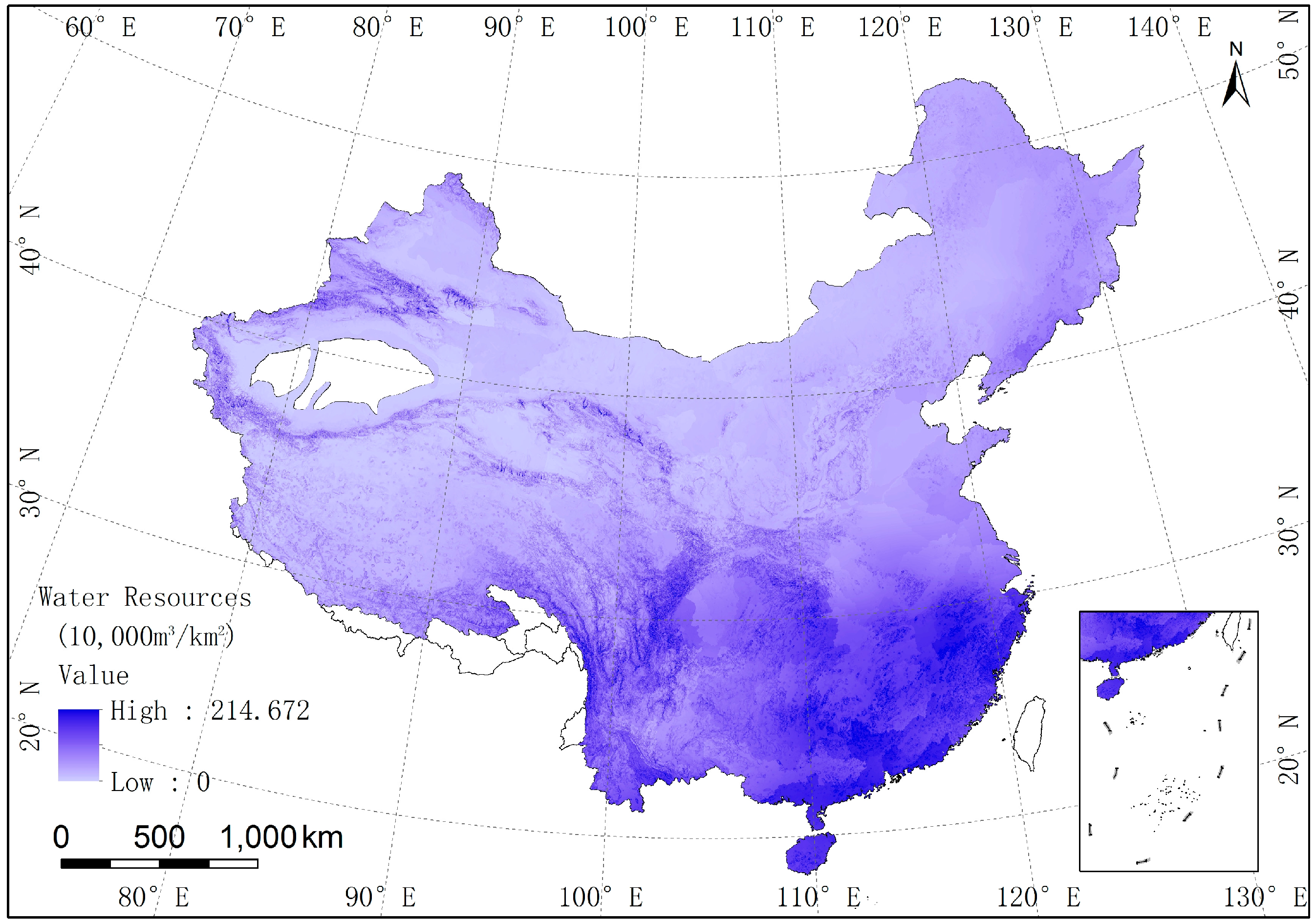
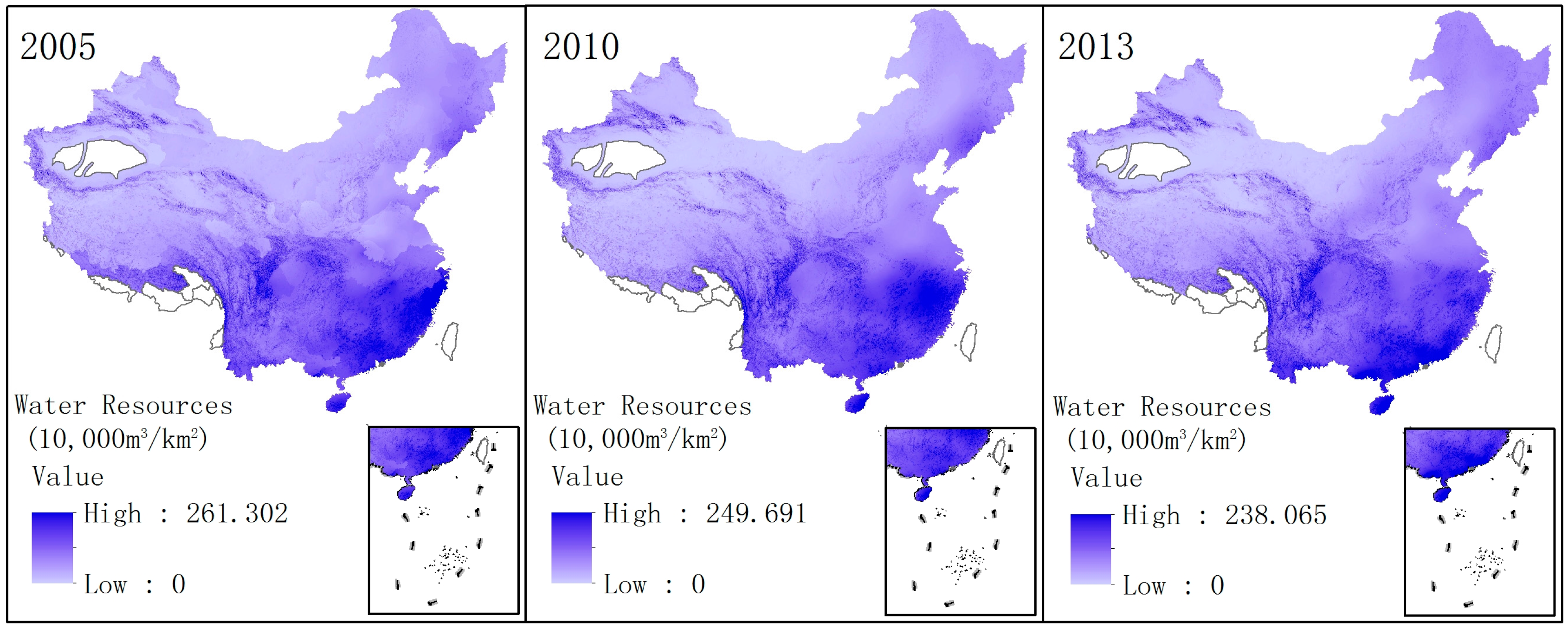
3.3. Gridded Water Resources Distribution Simulation

We applied model 2 to simulate water resources distribution at 1 km × 1 km grid scale in China. The model can be expressed as:

$${\widehat{y}}_i=-12.687+0.052P_i+3.388S_i$$

(6)

$$\mathsf{\lambda }{w}_{ij}{\mathsf{\epsilon }}_i=0.662w_{ij}(y_i-{\widehat{y}}_i)$$

(7)

where ${\widehat{y}}_i$ refers to the water resources determined by factors of precipitation and slope, $\mathsf{\lambda }{w}_{ij}{\mathsf{\epsilon }}_i$ refers to the water resources determined by spatial association. According to the Equations (6) and (7), we used the raster calculator of ArcGIS to produce the gridded water resource distribution map (Figure 3).

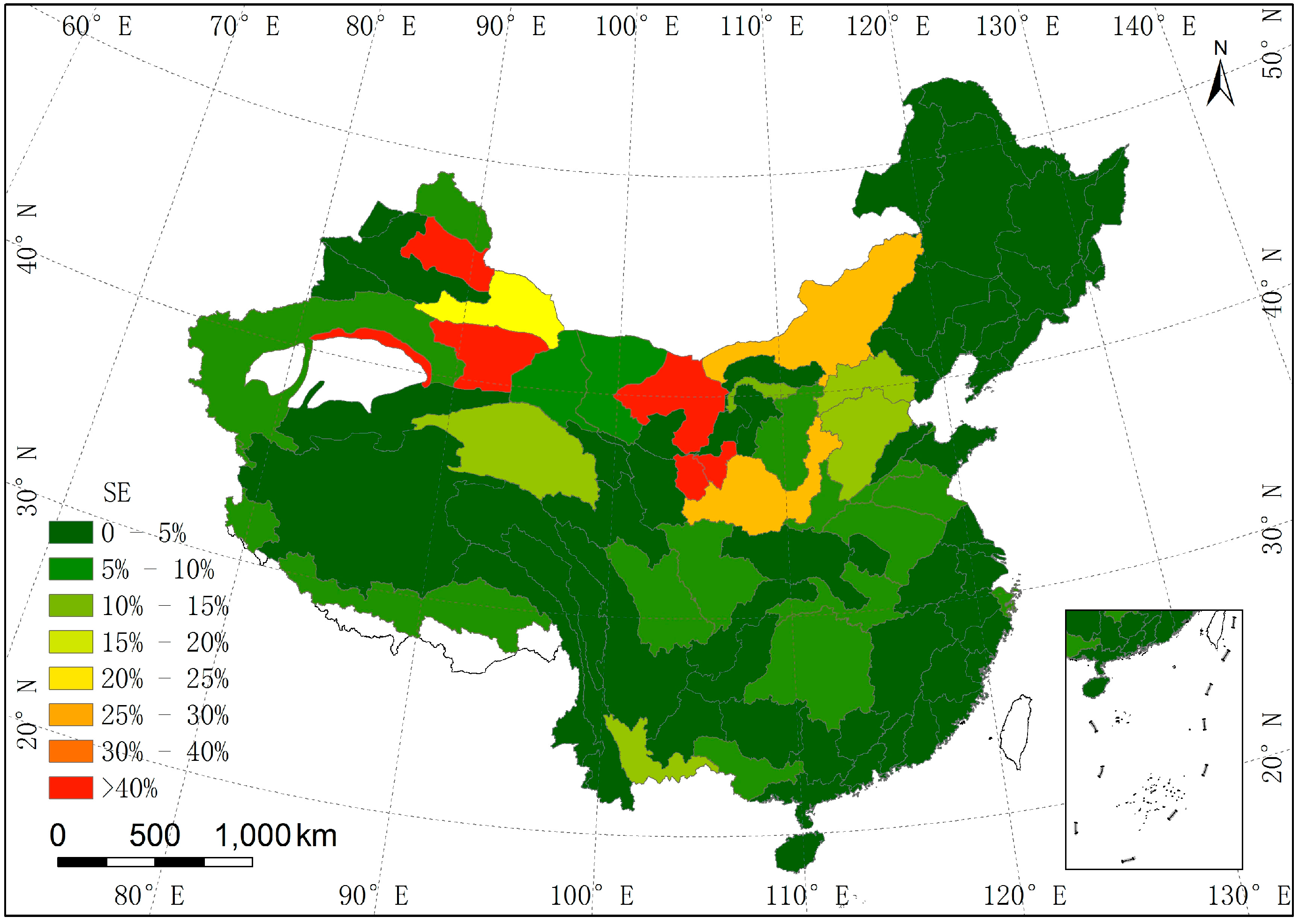
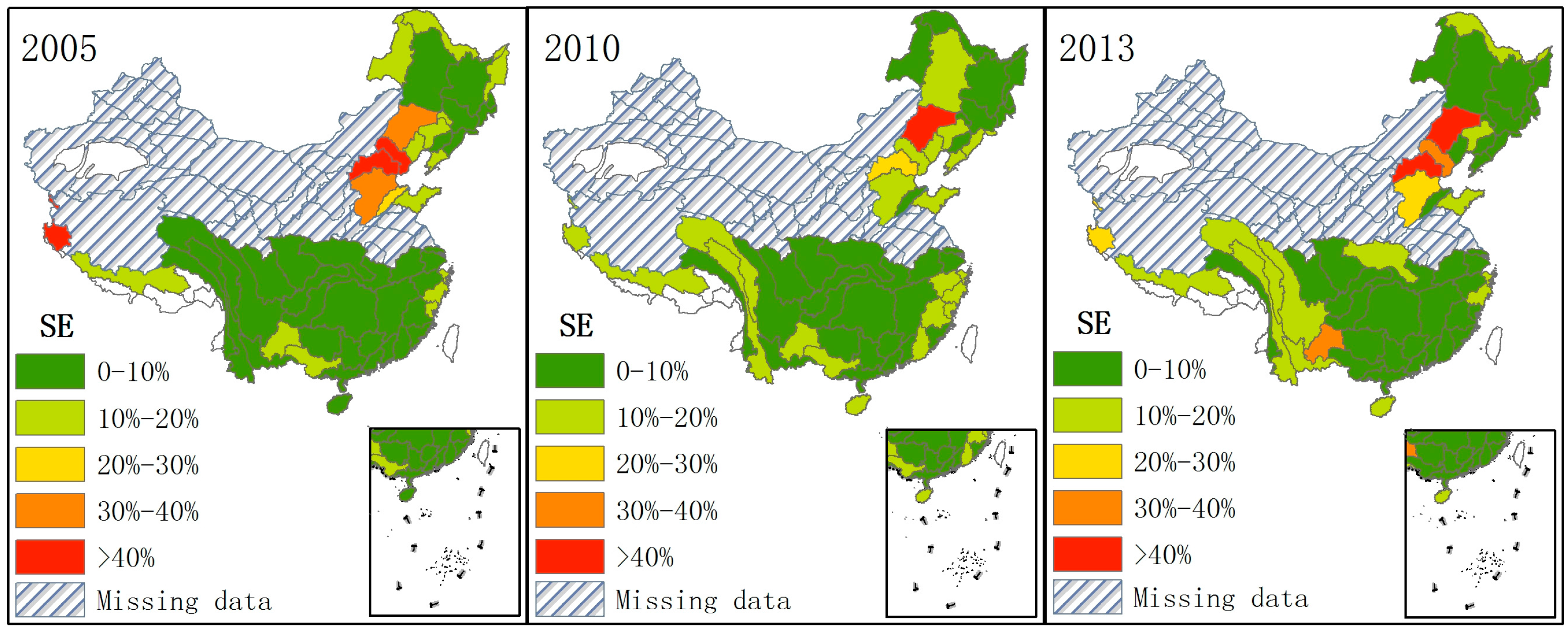
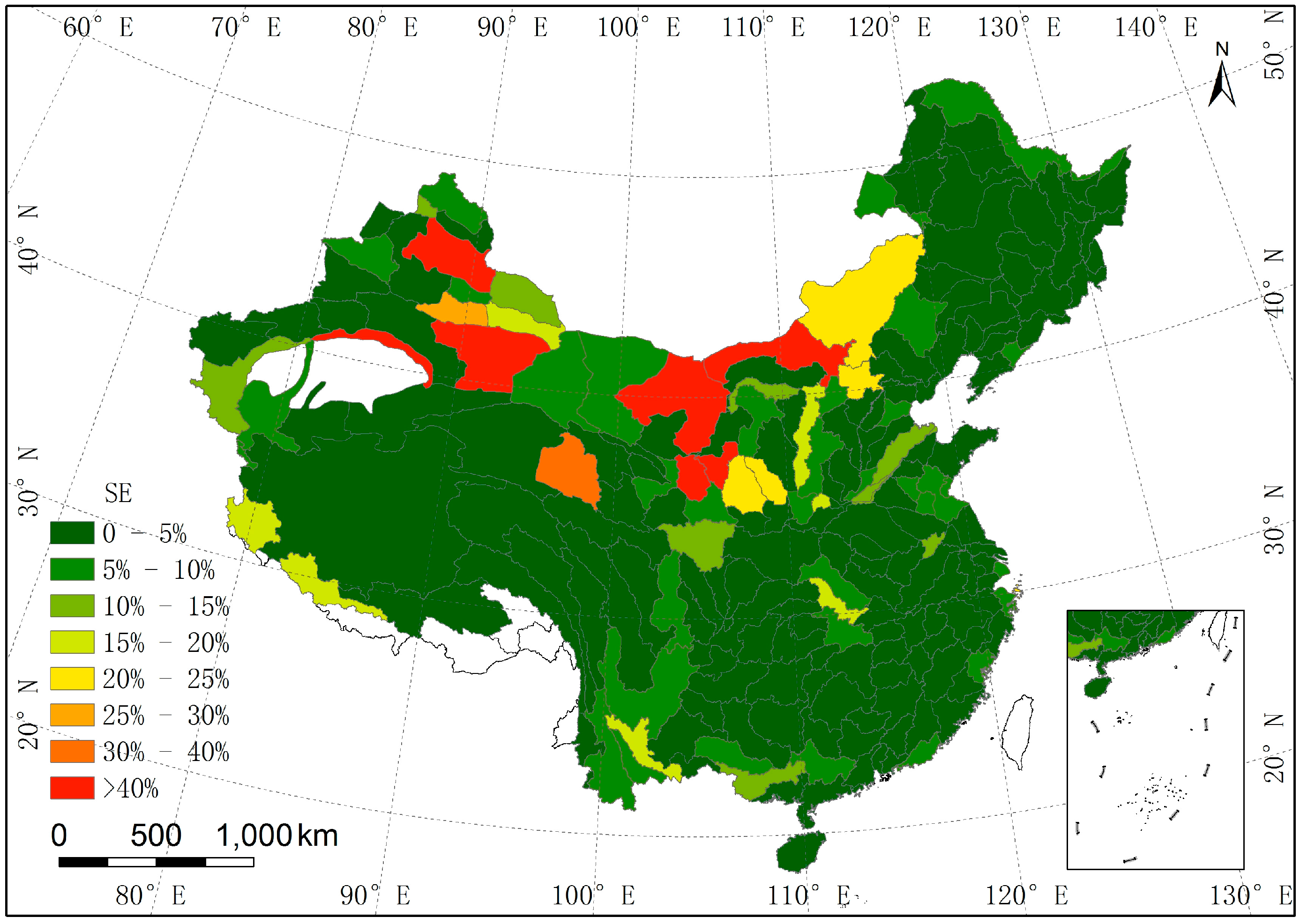
3.4. Accuracy Assessment for the Gridded Water Resource Distribution

Figure 4 shows the grade distribution of SE of the gridded water resources based on third-order basin. The SE of 140 third-order basins was lower than 5%. The SE of 35 third-order basins ranged from 5%–10%. The SE of 17 third-order basins ranged from 10%–20%. The SE of seven third-order basins ranged from 20%–30%. The SE of eight third-order basins was higher than 40%, and the eight third-order basins are located in extremely arid regions, such as Gurbantunggut Desert, Kumtag Desert, Hexi Desert, and the Tarim. Overall, the simulation accuracy of gridded water resource distribution for China in 2002 was very high.

In order to further verify the simulation results of gridded water resource distribution, we also calculated the sum of the gridded water resources within different second-order basins and offered the SE of the gridded water resources based on second-order basin (Figure 5). Among the 80 second-order basins, the SE of 51 second order-basins was lower than 5%. The SE of 15 second-order basins ranged from 5%–10%. The SE of seven second-order basins ranged from 10%–25%. The SE of five second-order basins was higher than 25%, and the five second-order basins are also located in extremely arid areas. Hence, the SE of the gridded water resource distribution in 2002 was stable in different scales of watershed. This indicated that the simulation results of gridded water resource distribution and accuracy assessment were both valid.

4. Discussion

The spatial autocorrelation model (model 2) shows that precipitation and slope were the two main factors influencing the amount of water resources. However, the impact of other factors (temperature, glacier, evapotranspiration, and forestland) on water resources were not significant. We needed to explain the results reasonably. Since precipitation is the main source of water resources, the water resources amount is influenced most by precipitation. Slope indirectly influences the regional amount of water resources by influencing the convergence of runoff.

Table 5. The correlation coefficient among the six independent variables.

Variable	Precipitation	Slope	Temperature	Glacier	Evapotranspiration	Forestland
Precipitation	1	0.014	0.839	–0.275	–0.141	0.719
Slope	0.014	1	–0.050	0.389	0.140	0.202
Temperature	0.839	–0.050	1	–0.215	–0.011	0.467
Glacier	–0.275	0.389	–0.215	1	0.495	–0.267
Evapotranspiration	–0.141	0.140	–0.011	0.495	1	–0.250
Forestland	0.719	0.202	0.467	–0.267	–0.250	1

shows the correlation coefficient among the six factors. The correlation coefficient between precipitation and slope was very low (0.014), which indicated that precipitation and slope were the two unrelated variables. The correlation coefficient between precipitation and temperature was very high (0.839). In reality, precipitation is distinctively affected by temperature. When precipitation has been included into the model, the effect of temperature on water resources was not significant. Glacier were one of the important sources of water resources. However, glacier only exists in the permafrost regions of Western China and has a high correlation with slope. Hence, the effect of glaciers on water resources was not significant. Forestland can increase the amount of regional water resources by the intercepting effect. However, forestland itself was influenced by precipitation and slope. The correlation coefficient between forestland and precipitation was also very high (0.719). Theoretically, evapotranspiration is the main factor to decrease the amount of water resources. Due to the complexity of the water cycle process, the effect of evapotranspiration on water resources was not significant in the model.

Though the R² was very high in the spatial error model (model 2 in Table 4), the quality of the model needed further evaluation. We offered the ordinary regression results acquired by a stepwise regression strategy without considering the autocorrelation of the spatial data (

Table 6. Estimates of the ordinary regression model by a stepwise regression strategy.

Dependent Variable: ${\mathit{y}}_{\mathit{i}}$	Model (7)	Model (8)	Model (9)	Model (10)	Model (11)	Model (12)
${\mathsf{\beta }}_0$ (t)	–6.084 (–4.400)	–12.789 *** (–8.698)	–12.693 *** (–8.720)	–12.600 *** (–8.743)	–14.205 *** (–8.286)	–14.259 *** (–8.176)
$P_i$ (t)	0.052 *** (39.137)	0.052 *** (44.668)	0.049 *** (29.118)	0.044 *** (15.286)	0.044 *** (15.429)	0.044 *** (15.392)
$S_i$ (t)		3.133 *** (8.007)	2.877 *** (7.142)	2.893 *** (7.253)	2.739 *** (6.730)	2.772 *** (6.197)
$T_i$ (t)				0.456 *** (2.282)	0.408 *** (2.031)	0.405 ** (2.010)
$G_i$ (t)						–0.001 (–0.181)
$E_i$ (t)					0.00008 (1.709)	0.00009 (1.616)
$F_i$ (t)			0.0009 *** (2.304)	0.0013 *** (2.968)	0.0014 *** (3.278)	0.0014 *** (3.202)
R2	0.8824	0.9107	0.9130	0.9444	0.9164	0.9164
LogL	–801.34	–773.075	–770.40	–767.77	–766.28	–766.26
AIC	1606.69	1552.15	1548.81	1545.54	1544.55	1546.52
SC	1613.34	1562.13	1562.12	1562.18	1546.52	1569.81

Notes: Levels of significance are reported as *** p < 0.01, ** p < 0.05 and * p < 0.1.

). According to statistical test, model 10 was better than the other models (model 7, model 8, model 9, model 11, and model 12) in Table 6 because of a higher R² and a statistical significance. However, compared with model 2 in Table 4, R² and LogL in model 10 were both lower than those in model 2. The values of AIC and SC were both higher than those in model 2. Overall, the SEM (model 2) was better than all six ordinary regression models, which also indicated that the spatial autocorrelation cannot be ignored when using geospatial data to build a model.

Apart from the quality of the model 2, we also needed to verify the simulation accuracy of gridded water resource distribution in China. We compared Figure 3 (the gridded water resource distribution map) with Figure 1 (water resource distribution map of third-order basins). From Figure 3, the simulation values of water resources in grid-cell of 1 km × 1 km ranged from 0–214.672. As a whole, the gridded water resource distribution was similar with the water resource distribution of third-order basins. Eastern regions of China have much water than the western regions; southern regions of China have much water than the northern regions; high vegetation-covered regions have much water than low vegetation-covered regions; the amount of water resources in desert areas of Northwestern China is close to 0.

Since no previous studies have been implemented to reveal the water resource distribution at such a fine scale, we cannot compare the research results with other related studies completely. Hence, though the simulation accuracy of gridded water resources distribution for China in 2002 was very high, we also needed to further verify the research results. We applied model 2 to simulate the gridded water resource distribution in 2005, 2010, and 2013. The simulation results (Figure 6) indicated that the spatiotemporal patterns of gridded water resource distribution in 2005, 2010, and 2013 were similar to that in 2002. It demonstrated that the gridded water resource distribution produced by the model 2 was stable, which also indicated that the result of gridded water resource distribution in 2002 was valid, to some degree.

Apart from the simulation maps of the gridded water resources distribution in 2002, 2010, and 2013, we also conducted the accuracy assessment for the simulation results of gridded water resource distribution. Due to the availability of data, the validation can only be implemented in second-order basins using statistical data of water resources from 2005, 2010, and 2013. Among the 80 second-order basins, the statistical data of water resources of 27 second-order basins were missing and only 53 second-order basins could be used to test the simulation accuracy. The simulation error of gridded water resource distribution for the three years is seen in Figure 7. In Figure 7, the SE of over 50% of the second-order basins was lower than 10%, and the SE of over 25% second-order basins ranged from 10%–20%. The simulation accuracies of the gridded water resources distribution in 2005, 2010, and 2013 were also very high.

Through the comparison of the SE of gridded water resources distribution (Figure 4, Figure 5 and Figure 7), we could find that the SE of the gridded water resources was very high in extremely arid regions, especially in some desert areas. We offer the distribution map of deserts in China (Figure 8). It is obvious that the areas with higher SE are mainly located in desert regions. In these desert regions, the yearly precipitation is less than 50 mm and the evapotranspiration is much higher than precipitation. The water resources in those areas mainly derives from groundwater replenishment from glacial melt water and surface water is distributed irregularly. The average water resources per square kilometer in third-order basins are approximately zero in those areas. Hence, the simulation of gridded water resource distribution in those areas with high SE is complicated and needs further research in the future. On the whole, the simulation result of gridded water resource distribution in 2002 was valid.

5. Conclusions

In this paper, the water resource distribution of China in 2002 was simulated at a 1 km × 1 km grid cell. We first tested the spatial autocorrelation of water resource data of third-order basins using Moran’s I index. Results show that there was a significant spatial autocorrelation among water resource data of third-order basins in China. Northern China had low-value clustering areas of water resources and Southeast China had high-value clustering areas of water resources.

The estimation results of the spatial autocorrelation model demonstrated that precipitation and slope were the main factors influencing the amount of water resources. The impact of temperature, glacier, evapotranspiration, and forestland on water resources was not significant. We gave a detailed analysis on the results of the model in the discussion section. In addition, we compared the spatial autocorrelation model with the ordinary regression model. The spatial autocorrelation model was better than the ordinary regression model in simulating the relationship between the water resources and the associated factors. Finally, we applied the valid spatial autocorrelation model to simulate the water resource distribution in grid-cells of 1 km × 1 km.

In addition, we also discussed the simulation accuracy of water resource distribution by calculating the relative error. The simulation accuracy of the gridded water resource distribution was very high, apart from some extremely arid regions (Gurbantunggut Desert, Kumtag Desert, and Hexi Desert). We also verified the effectiveness of the simulation result for the gridded water resources in 2002 by applying the model to estimate the gridded water resource distribution in 2005, 2010, and 2013. The raster data of the gridded water resource distribution in 2002 will provide more useful information for regional water resource management, and the data can also be used as an important data source in many research applications, such as the bearing capacity of water resources.

References

1. Gao, X.; Yu, T.F. The temporal-spatial variation of water resources constraint on urbanization in the northwestern China: Examples from the Gansu section of west Longhai-lanxin economic zone. Environ. Earth Sci. 2014, 71, 4029–4037. [Google Scholar] [CrossRef]
2. Bao, C.; He, D.M. The causal relationship between urbanization, economic growth and water use change in provincial China. Sustainability 2015, 7, 16076–16085. [Google Scholar] [CrossRef]
3. Liu, C.M.; Yu, J.J.; Kendy, E. Groundwater exploitation and its impact on the environment in the north China plain. Water Int. 2001, 26, 265–272. [Google Scholar]
4. Bao, C.; Fang, C.L. Water resources constraint force on urbanization in water deficient regions: A case study of the Hexi Corridor, arid area of NW China. Ecol. Econ. 2007, 62, 508–517. [Google Scholar] [CrossRef]
5. Jiang, Y. China’s water scarcity. J. Environ. Manag. 2009, 90, 3185–3196. [Google Scholar] [CrossRef] [PubMed]
6. Yu, X.M.; Geng, Y.; Heck, P.; Xue, B. A review of China’s rural water management. Sustainability 2015, 7, 5773–5792. [Google Scholar] [CrossRef]
7. Young, R.A.; Bredehoeft, J.D. Digital-computer simulation for solving management problems of conjunctive groundwater and surface water systems. Water Resour. Res. 1972, 8, 533–556. [Google Scholar] [CrossRef]
8. Uhlenbrook, S. Biofuel and water cycle dynamics: What are the related challenges for hydrological processes research? Hydrol. Process. 2007, 21, 3647–3650. [Google Scholar] [CrossRef]
9. Carvallo, H.O.; Cassel, D.K.; Bauer, A. Water losses from an irrigated soybean field by deep percolation and evapotranspiration. Water Resour. Res. 1975, 11, 267. [Google Scholar] [CrossRef]
10. Guo, Y.; Shen, Y.J. Quantifying water and energy budgets and the impacts of climatic and human factors in the Haihe River Basin, China: 2. Trends and implications to water resources. J. Hydrol. 2015, 527, 251–261. [Google Scholar] [CrossRef]
11. Wasowski, J.; Lamanna, C.; Gigante, G.; Casarano, D. High resolution satellite imagery analysis for inferring surface-subsurface water relationships in unstable slopes. Remote Sens. Environ. 2012, 124, 135–148. [Google Scholar] [CrossRef]
12. Mace, R.E. Comment on “long-term (1930–2010) trends in groundwater levels in texas: Influences of soils, landcover, and water use” by Sriroop Chauduri and Srinivasulu Ale. Sci. Total Environ. 2015, 517, 259–262. [Google Scholar] [CrossRef] [PubMed]
13. Do, V.; Thomas-Agnan, C.; Vanhems, A. Accuracy of areal interpolation methods for count data. Spat. Stat. 2015, 14, 412–438. [Google Scholar] [CrossRef]
14. Sager, G. Areal interpolation for tidal streams. Beitr. Meereskd. 1975, 36, 85–94. [Google Scholar]
15. Wu, S.-S.; Qiu, X.; Wang, L. Population estimation methods in gis and remote sensing: A review. Gisci. Remote Sens. 2005, 42, 80–96. [Google Scholar] [CrossRef]
16. Xie, Z. A framework for interpolating the population surface at the residential-housing-unit level. Gisci. Remote Sens. 2006, 43, 233–251. [Google Scholar] [CrossRef]
17. Thorpe, W.R.; Rose, C.W.; Simpson, R.W. Areal interpolation of rainfall with a double fourier-series. J. Hydrol. 1979, 42, 171–177. [Google Scholar] [CrossRef]
18. D’Antona, G.; Seifnaraghi, N. Temperature distribution reconstruction by eigenfunction interpolation of boundary measurement data. IEEE Trans. Instrum. Meas. 2014, 63, 334–342. [Google Scholar] [CrossRef]
19. Silvan-Cardenas, J.L.; Wang, L.; Rogerson, P.; Wu, C.; Feng, T.; Kamphaus, B.D. Assessing fine-spatial-resolution remote sensing for small-area population estimation. Int. J. Remote Sens. 2010, 31, 5605–5634. [Google Scholar] [CrossRef]
20. Lo, C.P. Population estimation using geographically weighted regression. Gisci. Remote Sens. 2008, 45, 131–148. [Google Scholar] [CrossRef]
21. Montello, D.R.; Fabrikant, S.I.; Ruocco, M.; Middleton, R.S. Testing the first law of cognitive geography on point-display spatializations. In Spatial Information Theory. Foundations of Geographic Information Science; Lecture Notes in Computer Science; Springer: Berlin/Heidelberg, Germay, 2003; Volume 2825, pp. 316–331. [Google Scholar]
22. Qu, X.; Lee, L.F. Estimating a spatial autoregressive model with an endogenous spatial weight matrix. J. Econom. 2015, 184, 209–232. [Google Scholar] [CrossRef]
23. Shen, C.H.; Li, C.L.; Si, Y.L. Spatio-temporal autocorrelation measures for nonstationary series: A new temporally detrended spatio-temporal moran’s index. Phys. Lett. A 2016, 380, 106–116. [Google Scholar] [CrossRef]
24. Ma, W.; Ji, J.P.; Chen, P.; Zhao, T.T. Spatial-temporal patterns analysis of property crime in urban district based on Moran’s I and GIS. Inf. Technol. Comput. Appl. Eng. 2014, 253–258. [Google Scholar]
25. Epperson, B.K.; Li, T.Q. Measurement of genetic structure within populations using Moran’s spatial autocorrelation statistics. Proc. Natl. Acad. Sci. USA 1996, 93, 10528–10532. [Google Scholar] [CrossRef] [PubMed]
26. Anselin, L. Local indicators of spatial association—LISA. Geogr. Anal. 1995, 27, 93–115. [Google Scholar] [CrossRef]
27. Fu, W.J.; Jiang, P.K.; Zhou, G.M.; Zhao, K.L. Using Moran’s I and GIS to study the spatial pattern of forest litter carbon density in a subtropical region of southeastern China. Biogeosciences 2014, 11, 2401–2409. [Google Scholar] [CrossRef] [Green Version]
28. Cressie, N.; Collins, L.B. Patterns in spatial point locations: Local indicators of spatial association in a minefield with clutter. Nav. Res. Log. 2001, 48, 333–347. [Google Scholar] [CrossRef]
29. Zaman, G.; Goschin, Z. Economic downfall and speed of recovery in romanian counties. A spatial autoregressive model. Econ. Comput. Econ. Cybem. 2015, 49, 21–40. [Google Scholar]
30. Nankervis, J.C.; Savin, N.E. Testing the autoregressive parameter with the t statistic. J. Econom. 1985, 27, 143–161. [Google Scholar] [CrossRef]
Figure 1. The study area and China’s water resource distribution map of 206 third-order basins based on data from 2002. China contains 214 third-order basins. The data of eight third-order basins were invalid and those eight third-order basins were not selected as the study area.
Sustainability 08 01309 g001
Figure 2. The cluster maps of water resources in 2002 under the six spatial weights of: (a) first-order contiguity; (b) second-order contiguity; (c) third-order contiguity; (d) fourth-order contiguity; (e) fifth-order contiguity; and (f) sixth-order contiguity.
Sustainability 08 01309 g002
Figure 3. Gridded water resources distribution map of China (206 third-order basins) in 2002.
Sustainability 08 01309 g003
Figure 4. The grade map of the simulation error of the gridded water resource distribution based on third-order basin in 2002.
Sustainability 08 01309 g004
Figure 5. The grade map of the simulation error of the gridded water resource distribution based on second-order basin in 2002.
Sustainability 08 01309 g005
Figure 6. The gridded water resource distribution map in 2005, 2010, and 2013.
Sustainability 08 01309 g006
Figure 7. The grade distribution of simulation error (SE) water resources in second-order basins based on data from 2005, 2010, and 2013.
Sustainability 08 01309 g007
Figure 8. The distribution map of deserts in China.
Sustainability 08 01309 g008