Multi-Objective Optimization for Smart House Applied Real Time Pricing Systems

Abstract

A smart house generally has a Photovoltaic panel (PV), a Heat Pump (HP), a Solar Collector (SC) and a fixed battery. Since the fixed battery can buy and store inexpensive electricity during the night, the electricity bill can be reduced. However, a large capacity fixed battery is very expensive. Therefore, there is a need to determine the economic capacity of fixed battery. Furthermore, surplus electric power can be sold using a buyback program. By this program, PV can be effectively utilized and contribute to the reduction of the electricity bill. With this in mind, this research proposes a multi-objective optimization, the purpose of which is electric demand control and reduction of the electricity bill in the smart house. In this optimal problem, the Pareto optimal solutions are searched depending on the fixed battery capacity. Additionally, it is shown that consumers can choose what suits them by comparing the Pareto optimal solutions.

1. Introduction

Currently, power systems reform has been performed in Japan. In 2015, the Organization for Cross-regional Coordination of Transmission Operators (OCCTO) was established for the purpose of supply and demand adjustment of the national power transmission and distribution equipment, and in April 2016, full liberalization of retail electric power had started [1]. Therefore, the reduction of electricity prices will be expected due to the entry and competition of many new electric power companies [2]. Furthermore, smart meters, which can be checked remotely, will be installed, so in the future, it will be expected to construct a smart grid that can have a two-way communication with electric power demand in real time [3,4]. Consequently, it will be expected that Time Of Use (TOU) in addition to Real-Time Pricing (RTP) set one hour aheadwill be performed [5]. The RTP price becomes expensive in proportion to the demand of electric power, and therefore, Demand Response (DR) smooths the electric power demand. Actually, full liberalization of retail electric power has been performed in Illinois, USA, and there is an electric power retail company that provides RTP price for general consumers [6]. This company notifies consumers having a smart meter of the next day RTP price on the previous day. A consumer can reduce the electricity bill by modifying the time of electric appliance usage depending on the notified RTP price [7,8].

On the other hand, in the Conference of Parties 21 (COP21) in December 2015 in France, there was a motion to restrain the average temperature rise in the world [9]. To achieve a low-carbon society in reality, in addition to the conversion of liquefied natural gas, renewable energy power generation equipment, such as solar power generation equipment, has been attracting attention, and its development and widespread use are desired in the future to contribute to the local production for local consumption [10]. In Japan, it is possible to sell renewable energy generation power by the Feed-In Tariff (FIT). However, there is a tendency that the cost of renewable energy power generation equipment becomes less expensive, and there are FIT financial resources in addition to the electricity bill of consumers, so the purchase price by the FIT is reviewed annually and has a declining trend. Therefore, it is considered in the future that electricity will be sold at the electricity market price [11].

In this way, in the future of the power distribution system, it is assumed that electricity trading will be performed mainly in the electricity market. However, electric power in the electricity market is traded in proportion to the power demand. Therefore, there is need to decrease the electricity market price and the electricity bill price and to improve the economy [12,13,14]. A smart house can regulate the power demand by being associated with a smart grid [15,16,17,18]. When this operation method is performed, controllable loads, like a fixed battery and Heat Pump (HP), are used, so it is possible to adjust. However, since the power consumption of appliances depends on the use plan and contracted power, this is difficult to modify. Therefore, many research works on the optimization of energy management, which imposes a penalty for the planning of power consumption management, have been carried out using the multi-objective optimization method [19,20]. In [19,20], a penalty for the usage plan adjustment of electric appliances has been introduced, and the electricity bill can be reduced by using the DR. However, as a problem in this research, the unit of penalty has not been generalized. Furthermore, a case that introduces renewable energy power generation equipment like PV is not considered. Therefore, a new multi-objective optimization algorithm is required, which includes the DR, a generalized penalty index and a smart house with renewable sources.

In this research, multi-objective optimization for a smart house applying RTP as DR is proposed. For the assumed smart house, PV, the Solar Collector (SC), in addition to controllable loads, like HP and a fixed battery, are introduced. Furthermore, electricity is purchased at the RTP price, and the surplus power of renewable energy is sold at the RTP price. The owner of a smart house can modify the usage time of the electric appliances considering the RTP price. Therefore, a multi-objective optimization technique is proposed to minimize the regulation effort of the electricity appliances and electricity cost. By this simulation, it is possible to plan the use time of the electric appliances and the operation method of controllable loads. Moreover, in this simulation, the Pareto optimal front is compared for different cases of the capacity of the fixed battery. Evaluating the Pareto optimal front, the effect of the reduction of the regulation effort and electricity bill cost by increasing the capacity of the fixed battery is shown.

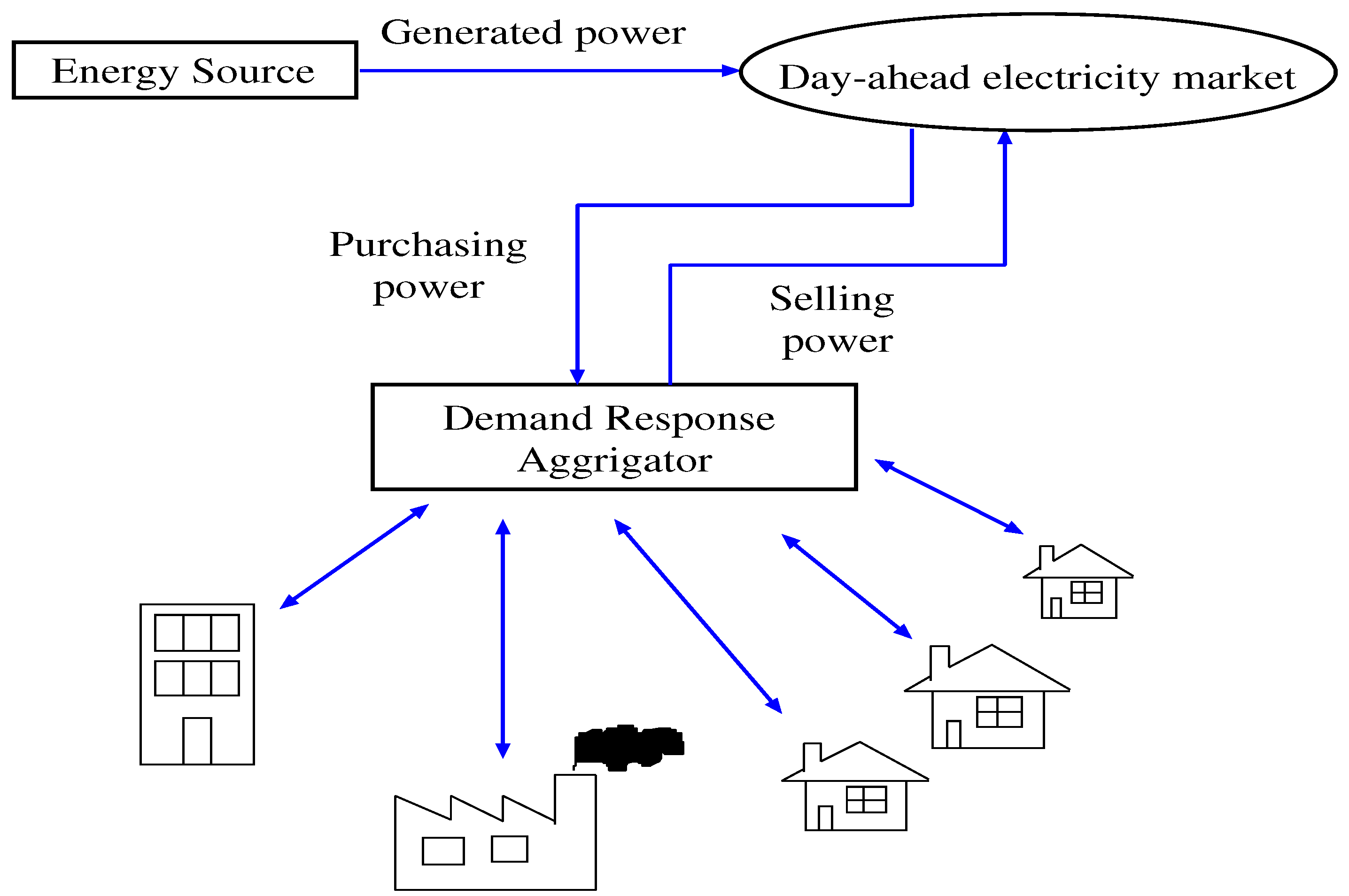
2. Power System Model

The schemes of the smart community and power trading are shown in Figure 1 and Figure 2, respectively. As illustrated in Figure 1 and Figure 2, customers constitute the smart community, and the RTP price is announced based on the electricity market price of the previous day. Customers operate electric appliances (i.e., different loads) based on the RTP price from the DR aggregator. The DR aggregator performs its business using expected demand data [21]. This research focuses on a customer participating in this smart community. In this section, the structure of the system introduced in the smart house is explained. Section 2.1, Section 2.2, Section 2.3 and Section 2.4 describe the assumed smart house model, supply-demand balance of the smart house, the PV system and the water heating system.

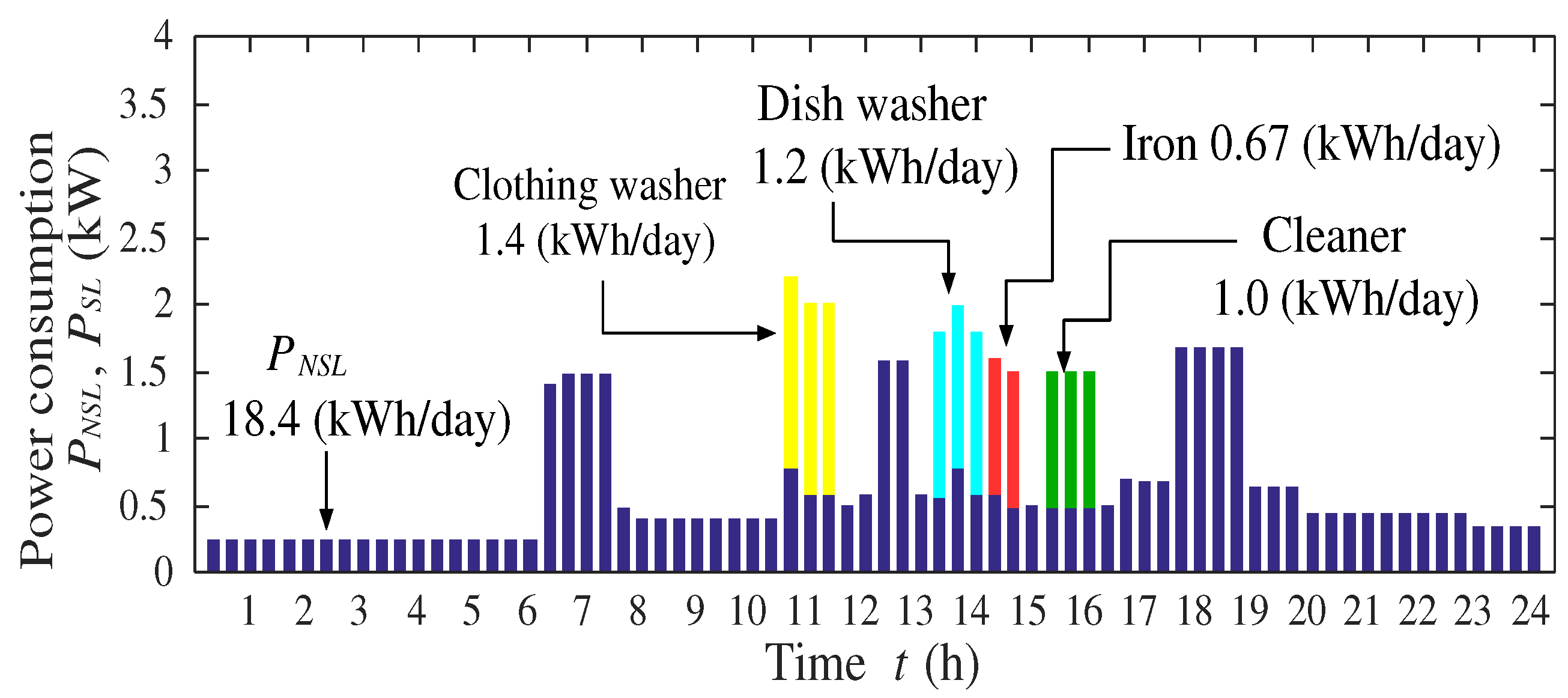
2.1. Smart House Model

The smart house model used in this research is illustrated in Figure 3 [22]. PV, SC and HP are introduced into this model. It is assumed that hot water is used in the morning and evening times. Target temperatures are 50 ${}^{\circ }\mathrm{C}$ and 60 ${}^{\circ }\mathrm{C}$ at 6:00 a.m. and 19:00 p.m. for the storage tank’s water. If the hot water temperature in the storage tank is lower than the target temperature, HP heats the water to the target temperature. Regarding HP, the rated heating capacity is 1 kW/4 kW; the value of COP is 4.0; and the hot water storage capacity is 370 L.

2.2. Supply-Demand Balance of the Smart House

$P_{It}$, $P_{Lt}$, $P_{PVt}$, $P_{BAt}$ and $P_{HPt}$ in Figure 3 represent the interconnection point of power flow (kW), the power consumption excluding controllable loads (kW), PV generator output (kW), discharge and charge power of fixed battery (kW) and the power consumption of the HP (kW). In Figure 3 of the smart house model, the following equations are described from the relationship between the supply and demand balance.

$$P_{It}=P_{Lt}+P_{HPt}-P_{PVt}-P_{BAt}$$

(1)

Furthermore, the value $P_{Lt}$ is constructed by shiftable loads $P_{SLt}$ and non-shiftable loads $P_{NSLt}$. Hence,

$$P_{Lt}=P_{SLt}+P_{NSLt}$$

(2)

In addition, the following equation sums up power consumption $P_{SLit}$ for shiftable electrical appliance i:

$$P_{SLt}=\sum _{i\in I}{P}_{SLit}$$

(3)

where I is a set of shiftable electrical appliances i.

Table 1. Electric appliances data.

Electric Appliance	Power Consumption (kW)	Use Time Zone
Refrigerator	0.25∼0.3	non-shiftable
Lighting	0.1∼0.5	load
IH (Induction Heating) cooking heater	0.2∼0.7	$P_{NSLt}$ (kW)
TV	0.085
Air conditioner	0.2∼0.4
Clothing washer	1.4	shiftable
Dish washer	1.2	load
Iron	1.2	$P_{SLt}$ (kW)
Cleaner	1.0

shows the shiftable electrical appliance and power consumption considered in this research. As listed in Table 1, non-shiftable loads are the refrigerator, lighting, IH (Induction Heating) cooking heater, television and air conditioner, and shiftable loads are the clothing washer, dish washer, iron and cleaner.

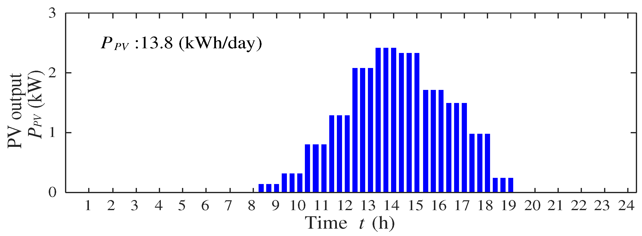
2.3. Photovoltaic System

In this research, the conversion efficiency of the solar cell array ${\eta }_{PV}$ is 14.4%; the number of panels $n_{PV}$ is 18 panels; the array area per panel $S_{PV}$ is 1.3 ${\mathrm{m}}^2$. When the amount of solar radiation $I_a(\mathrm{kW}/{\mathrm{m}}^2)$, PV output $P_{PV}\left(\mathrm{kW}\right)$ is calculated by the following equation [23].

$$\begin{array}{c}\hfill P_{PV}={\eta }_{PV}{n}_{PV}{S}_{PV}{I}_a(1-0.005(T_{CR}-25))\end{array}$$

(4)

Here, $T_{CR}{(}^{\circ }\mathrm{C})$ is the cell temperature, but this paper is using outside air temperature to simplify.

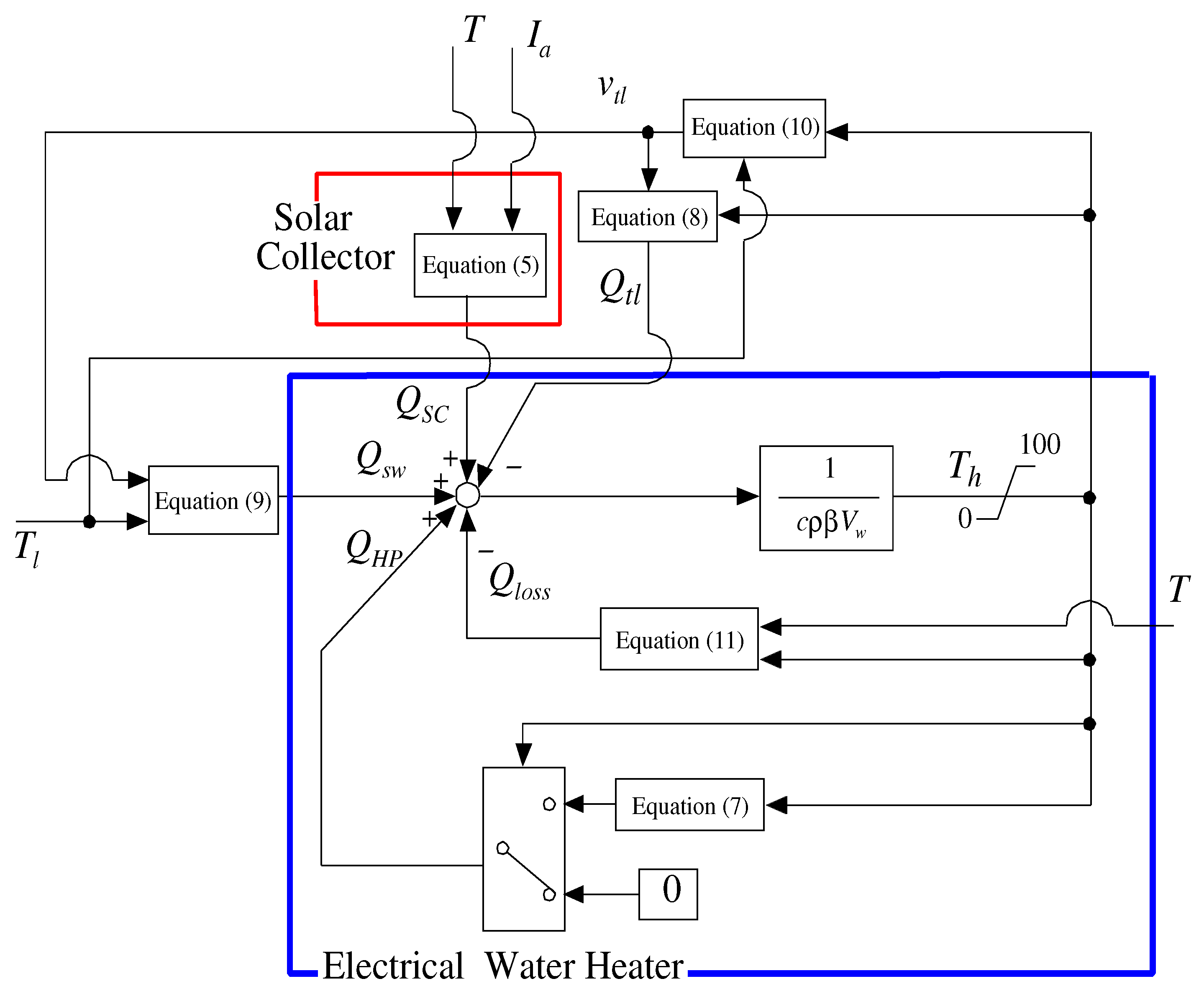
2.4. Solar Collector System

The model of the solar collector system is illustrated in Figure 4 [24,25,26]. The solar thermal energy obtained from the solar collector $Q_{SC}\left(\mathrm{kW}\right)$ is calculated by the following equation:

$$\begin{array}{ccc}\hfill Q_{SC}& =& \{F_R{\left(\tau \alpha \right)}_e{I}_a-F_R{U}_L(T_h-T)\}{S}_{SC}\hfill \end{array}$$

(5)

where $F_R$ is the heat removal efficiency, ($\tau \alpha$)${}_e$ is the effective transmission absorption factor, $U_L$ (kW/(${\mathrm{m}}^2{·}^{\circ }$C)) is the integrated solar thermal loss coefficient, $T_h{(}^{\circ }\mathrm{C})$ is hot water temperature in the storage tank, $T{(}^{\circ }\mathrm{C})$ is the outdoor temperature and $S_{SC}\left({\mathrm{m}}^2\right)$ is the solar collector area per collector ($S_{SC}={4.8}^{\circ }$). In Equation (5), the value $F_R{\left(\tau \alpha \right)}_e$ is 0.77; the value $F_R{U}_L$ is $5.0\times {10}^{-3}$ kW/(${\mathrm{m}}^2{·}^{\circ }$C). Furthermore, the angle of inclination of the panel is 30 degrees.

The temperature change and dynamic characteristics of the water in the storage tank can be expressed as:

$$\begin{array}{c}\hfill Q_{SC}+Q_{HP}-Q_{tl}+Q_{sw}-Q_{loss}=\beta A_w\frac{d{T}_h}{dt}\end{array}$$

(6)

$$\begin{array}{ccc}\hfill Q_{HP}& =& \beta A_w(T_d-T_h)\hfill \end{array}$$

(7)

$$\begin{array}{ccc}\hfill Q_{tl}& =& \beta v_{tl}{T}_h\hfill \end{array}$$

(8)

$$\begin{array}{ccc}\hfill Q_{sw}& =& \beta v_{sw}{T}_l\hfill \end{array}$$

(9)

$$\begin{array}{ccc}\hfill v_{tl}& =& v_{sw}\hfill \end{array}$$

(10)

$$\begin{array}{ccc}\hfill Q_{loss}& =& U_{st}(T_h-T)\hfill \end{array}$$

(11)

where $Q_{HP}\left(\mathrm{kW}\right)$ is the thermal energy from HP, $Q_{tl}\left(\mathrm{kW}\right)$ is the thermal energy for the hot water supply, $Q_{sw}\left(\mathrm{kW}\right)$ is the thermal energy from the water supply, $Q_{loss}\left(\mathrm{kW}\right)$ is the thermal energy of heat transmission between the hot water temperature in the storage tank and the outside temperature, β (kW/(L${·}^{\circ }$C)) is the volumetric specific heat of water, $A_w\left(\mathrm{L}\right)$ is the storage tank capacity, $t\left(\mathrm{h}\right)$ is time, $T_d{(}^{\circ }\mathrm{C})$ is the target temperature, $v_{tl}(\mathrm{L}/\mathrm{h})$ is the amount of used hot water from the storage tank, $v_{sw}(\mathrm{L}/\mathrm{h})$ is the amount of supplied water to the storage tank and $U_{st}\left(\mathrm{kW}{/}^{\circ }\mathrm{C}\right)$ is the heat loss coefficient of the storage tank between the storage tank and the outside temperature.

3. Optimization Method

In this section, the formulation of the multi-objective problem in this research and the optimization method are explained. Section 3.1 explains the regulation effort evaluation method; Section 3.2 describes the objective function and the constraint of the multi-objective problem; and Section 3.3 explains the multi-objective- optimization method.

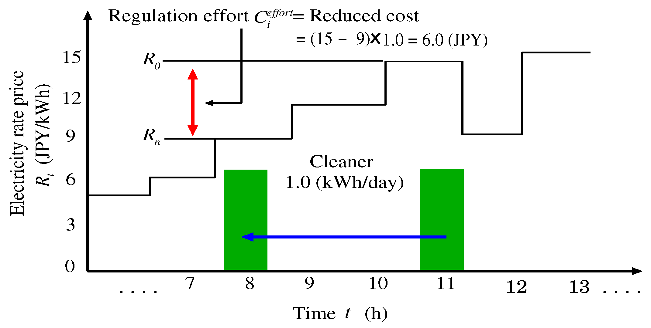
3.1. Regulation Effort Evaluation Method

Residents of the smart house can reduce the electricity bill by modifying the time of use of shiftable electric appliances. However, the electricity bill is not reduced by using the initial use plan. In this research, the residents of the houses can modify the usage plan of the electric appliances and reduce the electricity bill. This is know as the regulation effort of the electric appliances.

An example of the regulation effort is illustrated in Figure 5. As illustrated, the regulation effort is the reduced electricity cost for which the resident moves the block of power consumption of the electric appliances to the lower electric price time zone. On the other hand, when the resident moves to the higher price, the regulation effort is defined as zero. The regulation effort $C^{effort}$ of electric appliances i is expressed as the following equation:

$$C_i^{effort}=P_{SLit}(R_0-R_n)\Delta tif{R}_n\le R_0$$

(12)

where $P_{SLit}\left(\mathrm{kW}\right)$ is the power consumption of shiftable electric appliance i, $R_0(\mathrm{Yen}/\mathrm{kWh})$ is the RTP price by the initial use plan and $R_n(\mathrm{Yen}/\mathrm{kWh})$ is the RTP price by destination of the use time. The RTP price tends to be expensive at the electric demand peak time. Therefore, a large regulation effort is expected at the peak demand period.

3.2. Objective Functions and Constraints

The objective functions to be minimized are the electricity bill $E_{cost}\left(\mathrm{Yen}\right)$ and regulation effort $R_{effort}\left(\mathrm{Yen}\right)$ in the smart house and are expressed as the following equation:

$$MinimizeF\{E_{cost},R_{effort}\}$$

(13)

The objective functions are formulated as the following equations. In this research, the electric power selling price is the RTP price for simplification.

$$\begin{array}{ccc}\hfill E_{cost}& =& \sum _{t\in T}{R}_t(P_{Pt}-P_{St})\Delta t\hfill \end{array}$$

(14)

$$\begin{array}{ccc}\hfill R_{effort}& =& \sum _{i\in I}{C}_i^{effort}\hfill \end{array}$$

(15)

Here, $R_t(\mathrm{Yen}/\mathrm{kWh})$ is the RTP price; $P_{Pt}\left(\mathrm{kW}\right)$ is the purchased electric power; $P_{St}\left(\mathrm{kW}\right)$ is the sold electric power. Constraints on each piece of equipment are as follows:

$$\begin{array}{ccc}\hfill P_{PVt}& \le & P_{PV}^{\mathrm{rated}}\hfill \end{array}$$

(16)

$$\begin{array}{ccc}\hfill P_{It}& \le & P_{It}^{\mathrm{contact}}\hfill \end{array}$$

(17)

$$\begin{array}{ccc}\hfill |P_{It}-P_{I(t-1)}|& \le & P_{FB}\hfill \end{array}$$

(18)

$$\begin{array}{ccc}\hfill \left|P_{BAt}\right|& \le & P_{BA}^{\max }\hfill \end{array}$$

(19)

$$\begin{array}{ccc}\hfill 0.2C_{BA}^{\max }& \le & C_{BAt}\le 0.9C_{BA}^{\max }\hfill \end{array}$$

(20)

$$\begin{array}{ccc}\hfill \sum _{i\in I}{P}_{LSit}& \le & P_{LSi},i\in I\hfill \end{array}$$

(21)

Here, $P_{PV}^{\mathrm{rated}}$ is the PV rated output (3.5 kW); $P_{It}^{\mathrm{contact}}$ is the contract power (4.0 kW); $P_{FB}$ is the interconnection point power flow fluctuation range (2.0 kW); $P_{BAt}^{\max }\left(\mathrm{kW}\right)$ is the active power of the fixed battery; $P_{BA}^{\max }\left(\mathrm{kW}\right)$ is the maximum charge and discharge power of the fixed battery; $C_{BAt}\left(\mathrm{kWh}\right)$ is the state of charge for the fixed battery; $C_{BA}^{\max }\left(\mathrm{kWh}\right)$ is the fixed battery capacity maximum value. Equation (16) is the constraint on the maximum output power of the PV; Equation (17) is the constraint for buying power in the contract; Equation (18) is the constraint to limit sudden interconnection point power flow fluctuation. Equations (19) and (20) are constraints related to the fixed battery. At last, Equation (21) is the constraint to prevent the shiftable electric appliance i and the other appliances from being used at the same time.

3.3. NSGA2

Since there are two objective functions (i.e., minimization of the electricity bill and regulation effort), the Non-dominated Sorting Genetic Algorithm-2 (NSGA2) is used as a multi-objective optimization method. Many literature works about the multi-objective optimization method have been published by using NSGA2 [27,28,29].

In order to achieve an optimal Pareto solution, the crowding distance is considered in the same rank of the front, and it is the sum of the distances between the adjacent solution in each objective function [30]. The outline and the flow chart of NSGA2 is illustrated in Figure 6 and Figure 7 and is described below.

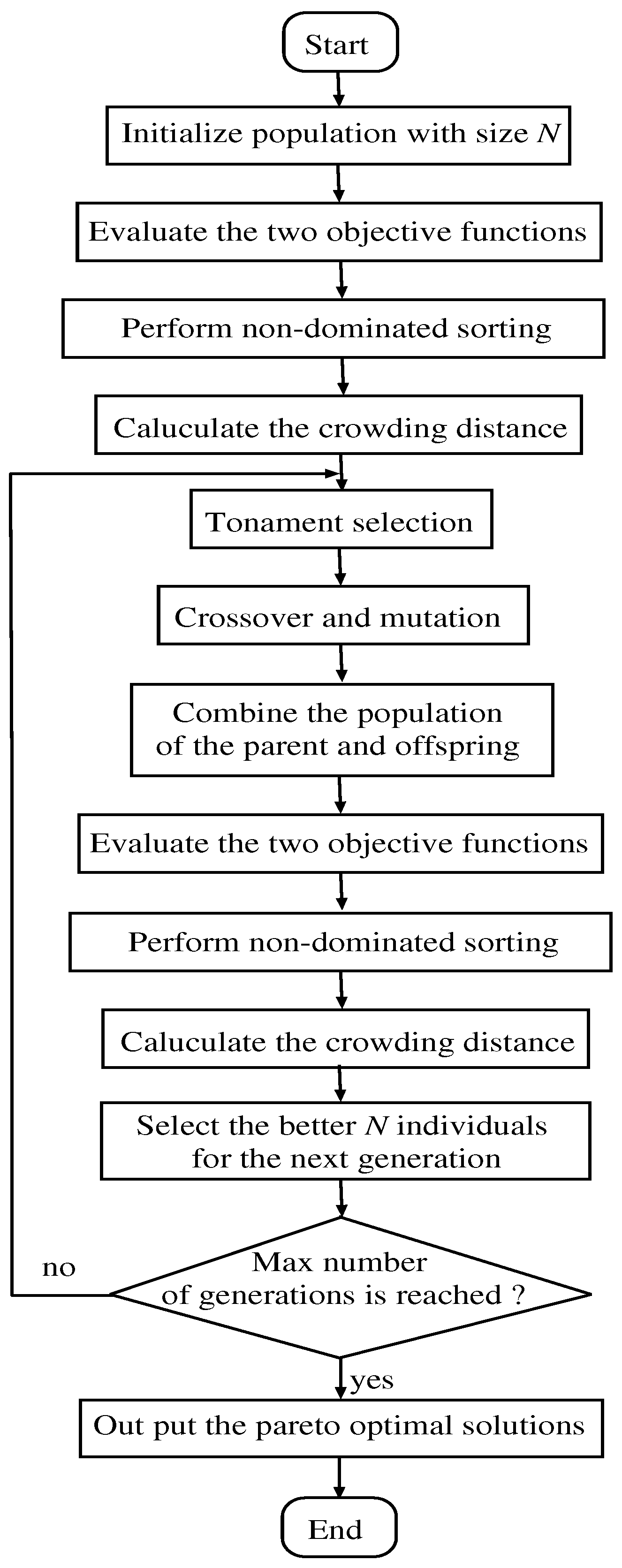
Step 1:

Making the initial population P of size N of the solution, P is the parent population.

Step 2:

Crossover and mutation are performed on the individual parent population, making the offspring population Q of size N.

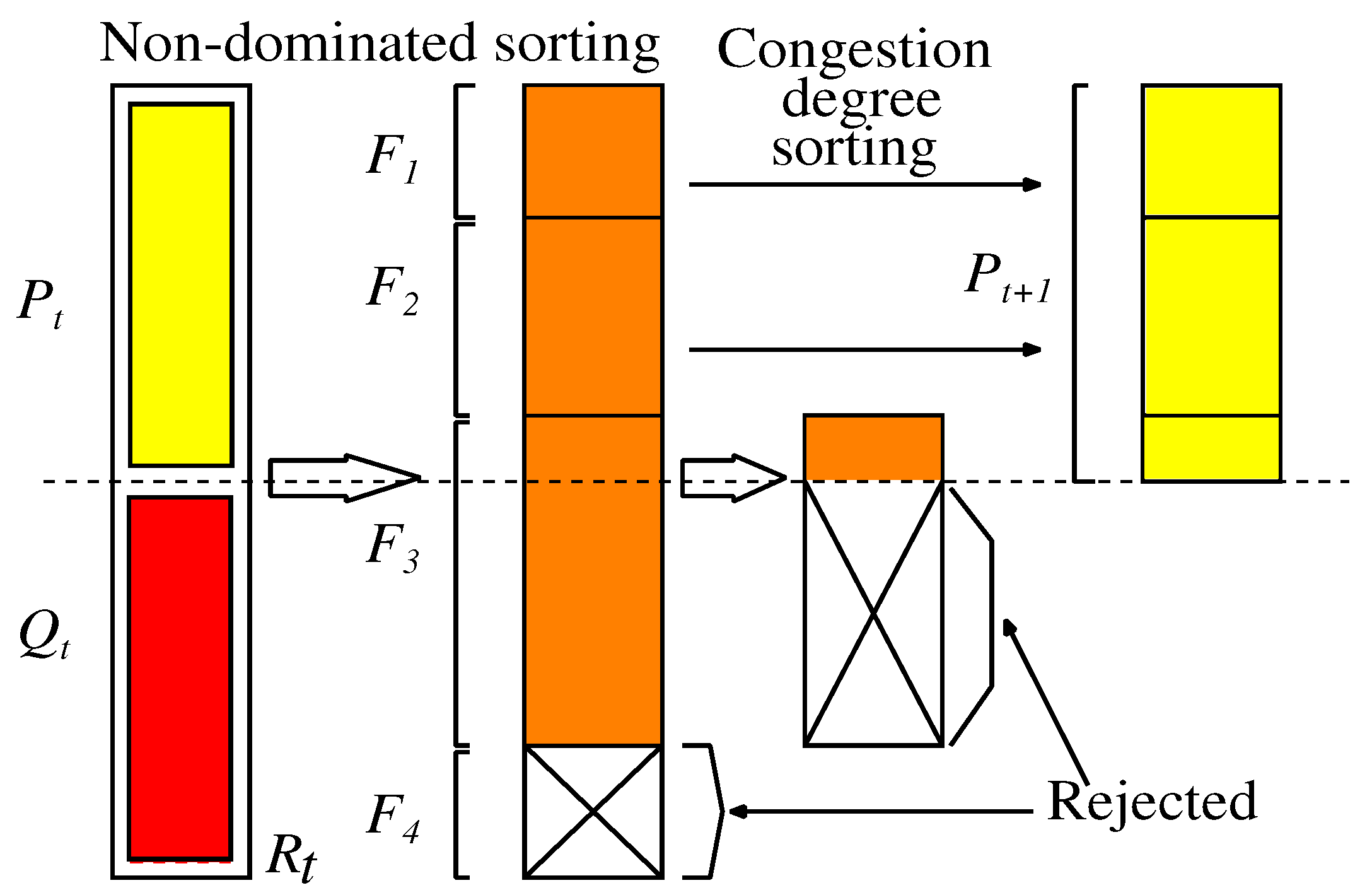
Step 3:

Combining the parent population P and the offspring population Q, R of size $2N$ is made.

Step 4:

R is Evaluated by the objective functions; the Pareto front is ranked by the non-dominated sorting.

Step 5:

The population is chosen till its size is N from the upper rank Pareto front; its population is the parent population in the next generation. If the number of the same rank Pareto front is over size N, a bad solution of diversity is deleted by crowding-distance computation.

Step 6:

If the generation reaches the max generation, the search is finished. Otherwise, the process returns to Step 2.

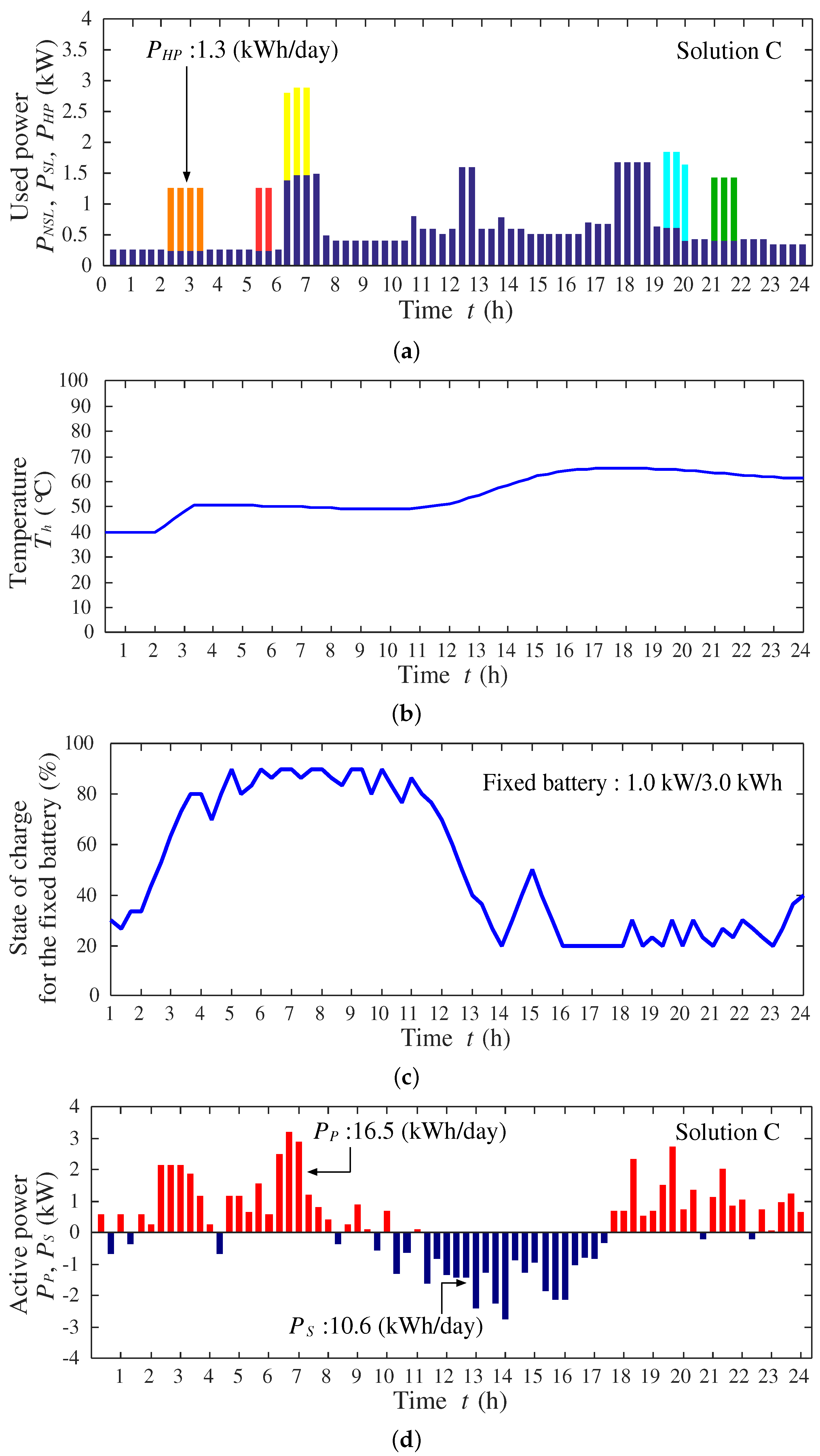
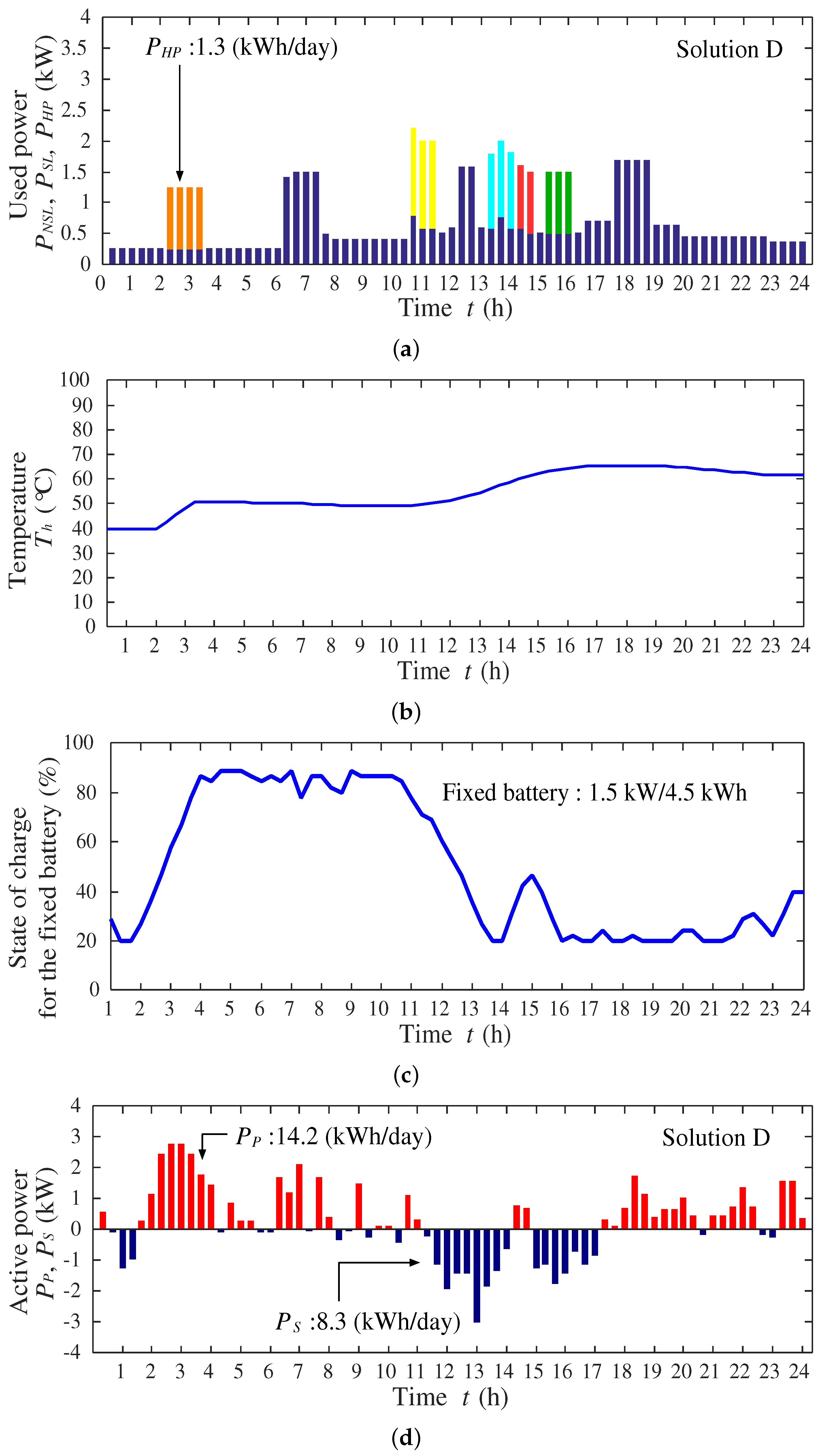
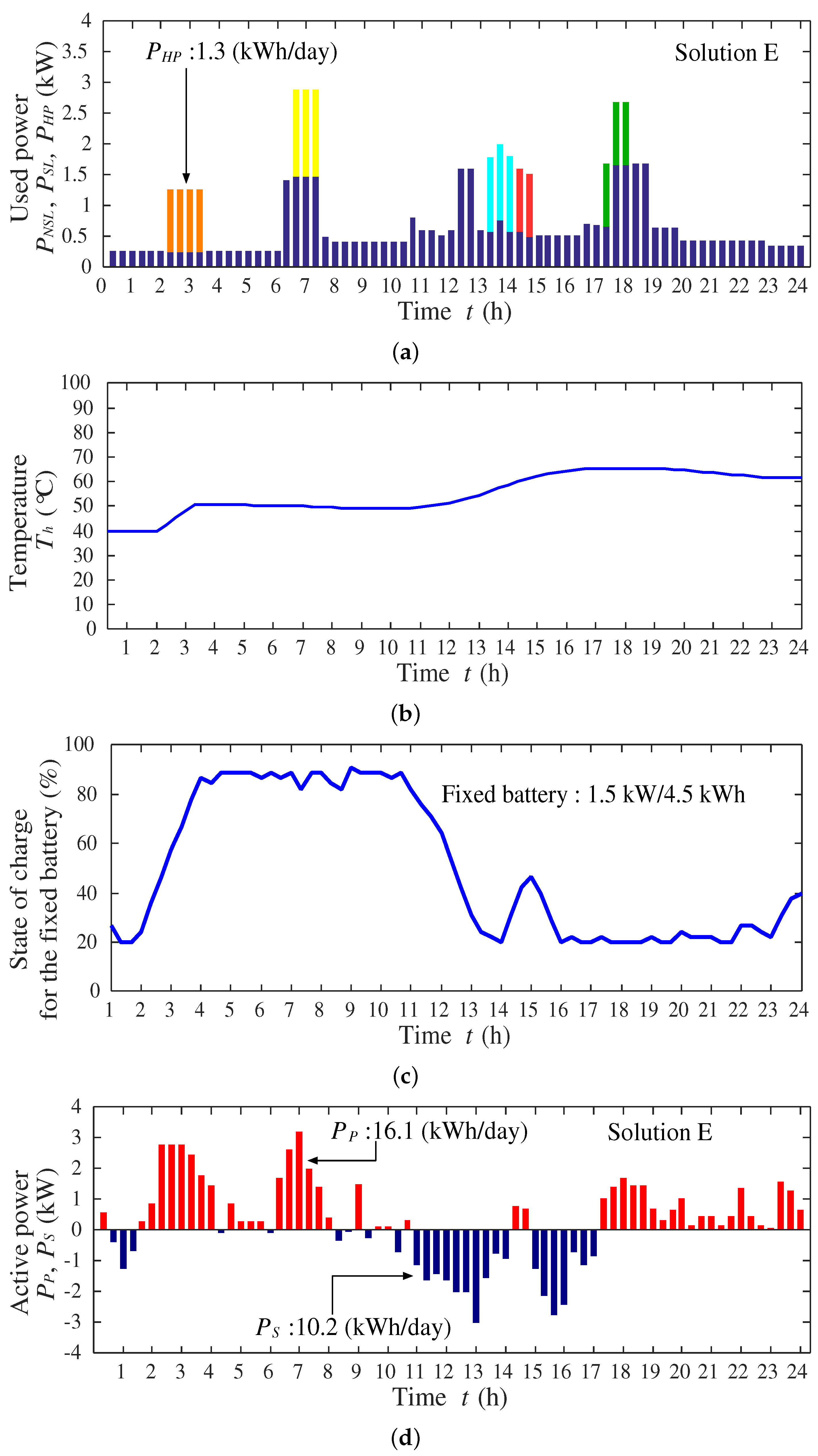
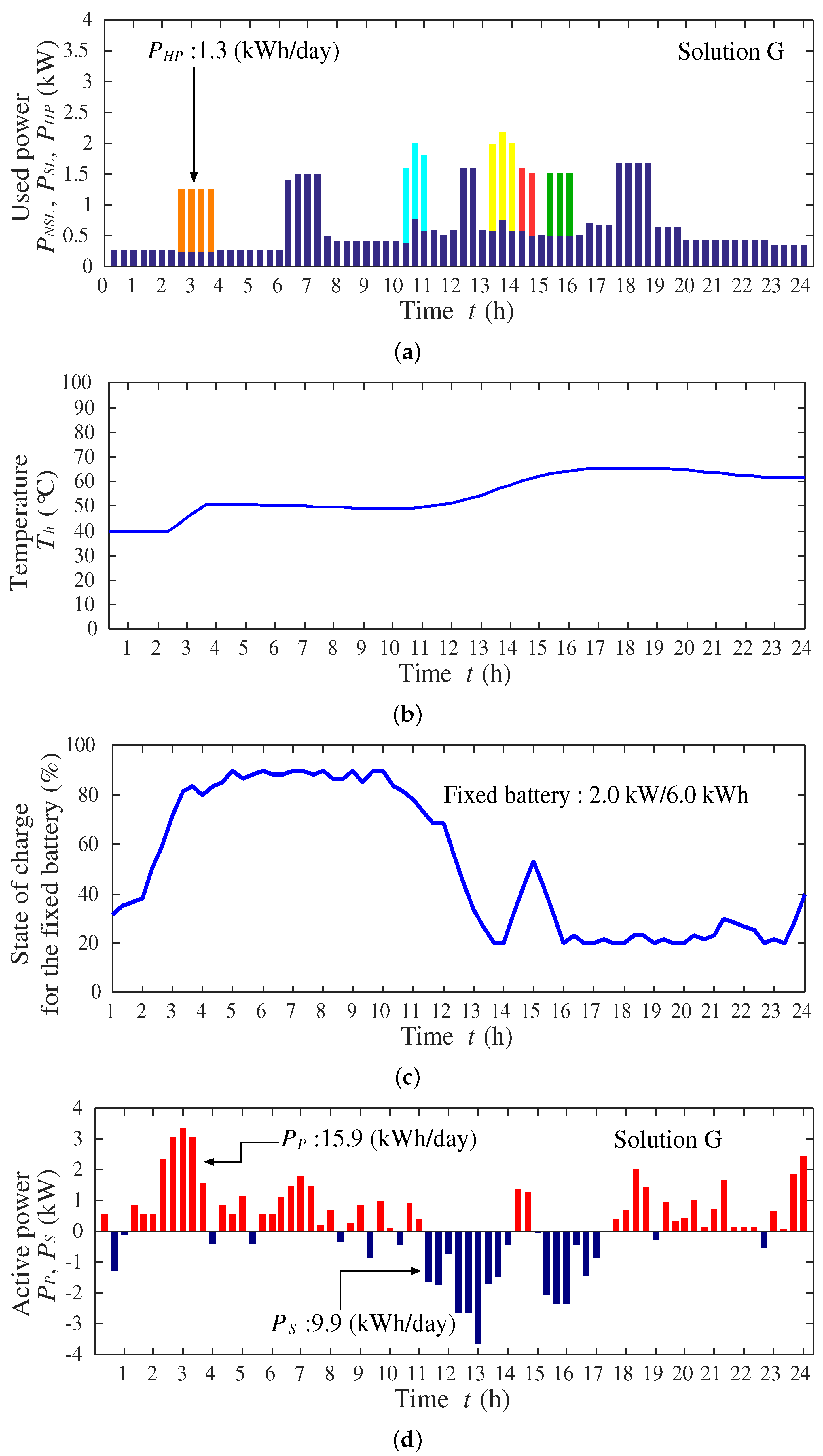
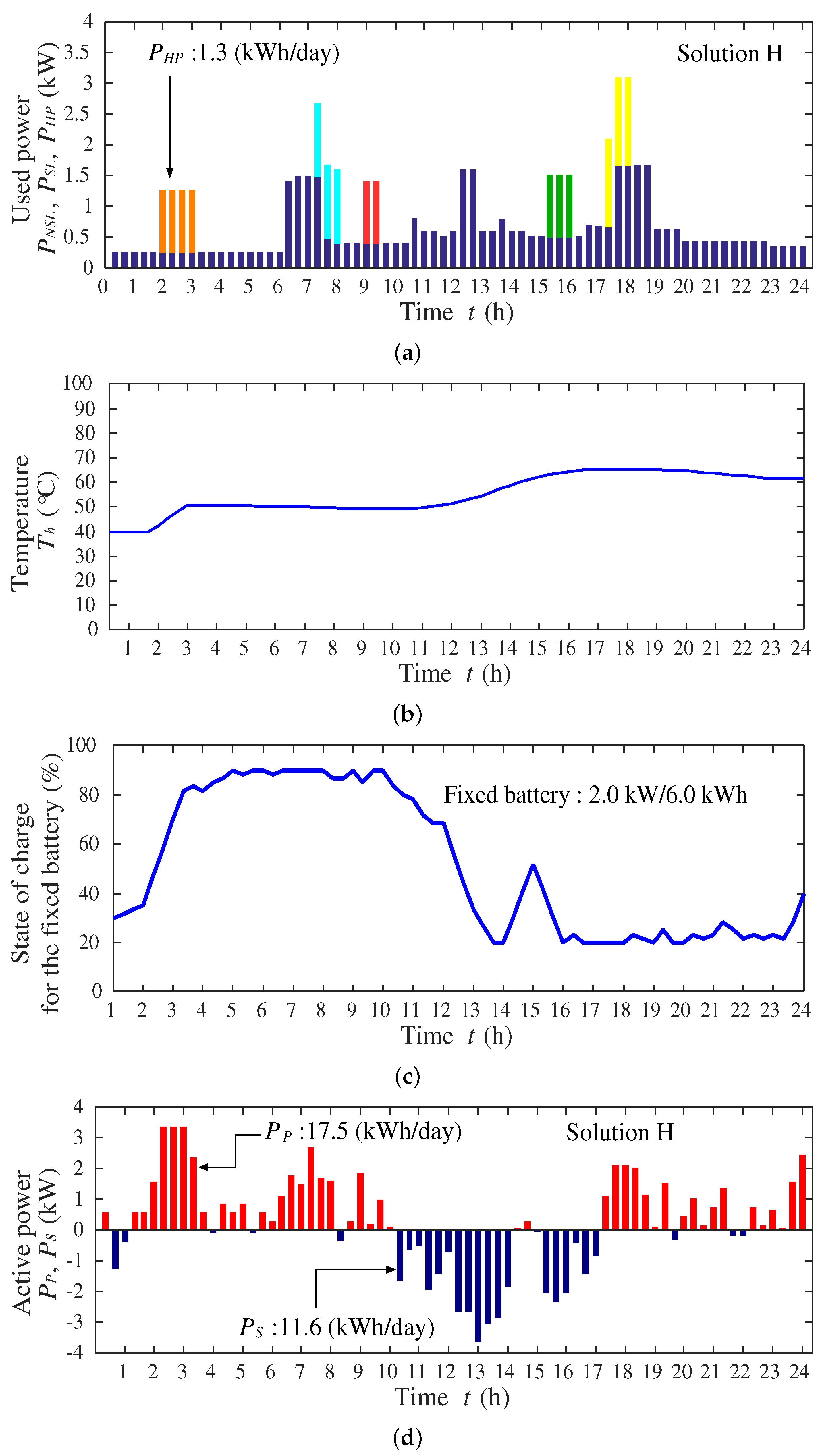
4. Simulation Results

In this section, the results of the simulation are considered. The simulation conditions are described in Section 4.1, and the discussion of the simulation results is described in Section 4.2.

4.1. Simulation Conditions

In this research, it is assumed that the simulation place is Naha city, Okinawa, in Japan. The assumed PV output power, initial usage schedule of the appliance in Table 1 and price of the RTP system of the next day are each illustrated in Figure 8, Figure 9 and Figure 10. Residents in the smart house move the time zone of the appliance in Figure 9 depending on the RTP price in Figure 10. Then, the reduced electricity bill cost is the regulation effort. Furthermore, in this research, 30 L and 150 L of hot water are used at 7∼8 a.m. and 7∼10 p.m. Moreover, if the hot water temperature is less than 50 ${}^{\circ }\mathrm{C}$ and 60 ${}^{\circ }\mathrm{C}$ at 7 a.m. and 8 p.m., the hot water is heated by HP. In this simulation, the electricity bill cost and regulation effort are compared by the difference in the capacity of the fixed battery. This comparison is performed for the cases of 1.0 kW/3.0 kWh, 1.5 kW/3.0 kWh and 2.0 kW/6.0 kWh. Here, 1.0 kW/3.0 kWh means the inverter capacity of the fixed battery is 1.0 kW, and the maximum capacity of the fixed battery is 3.0 kW.

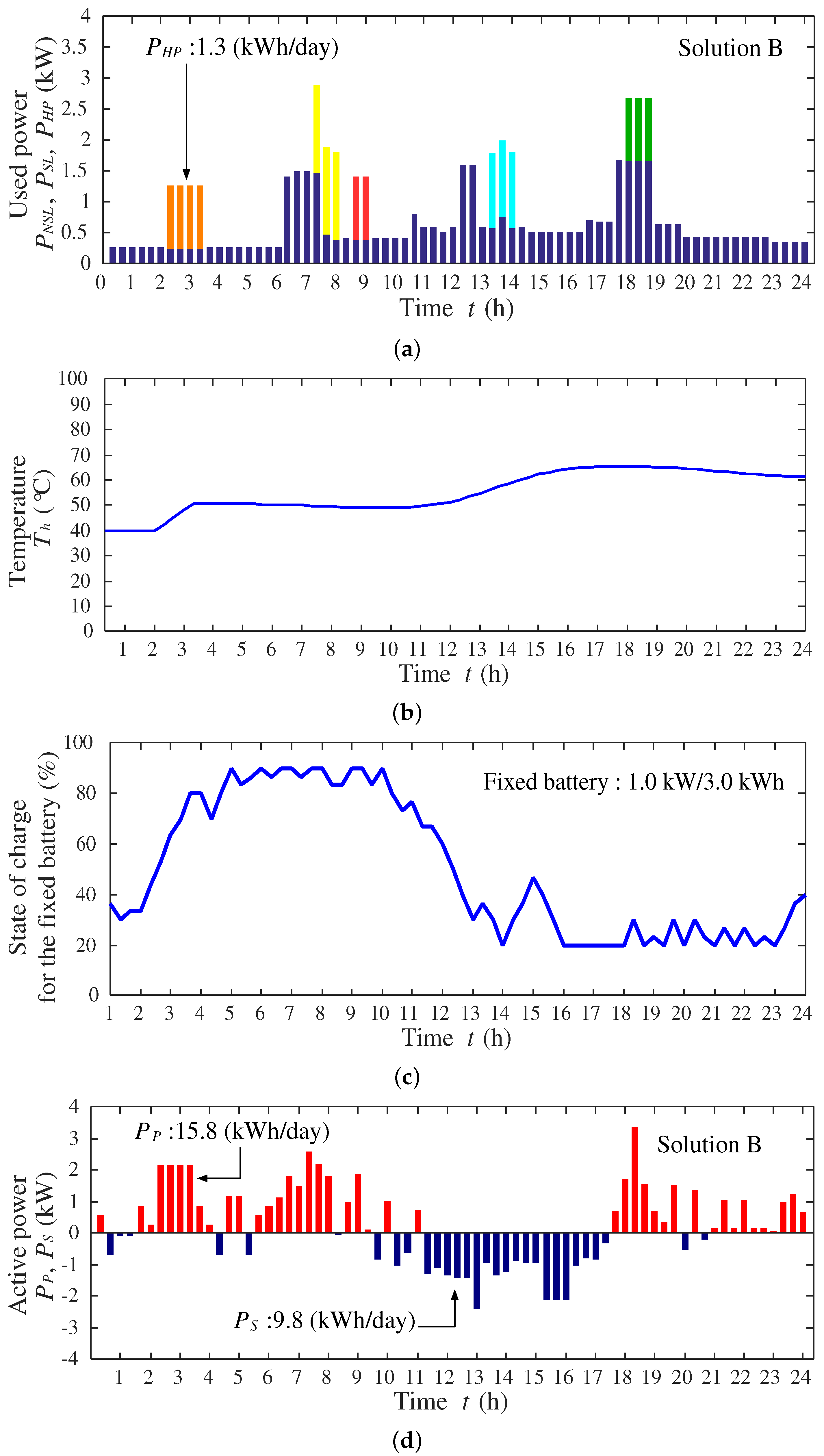
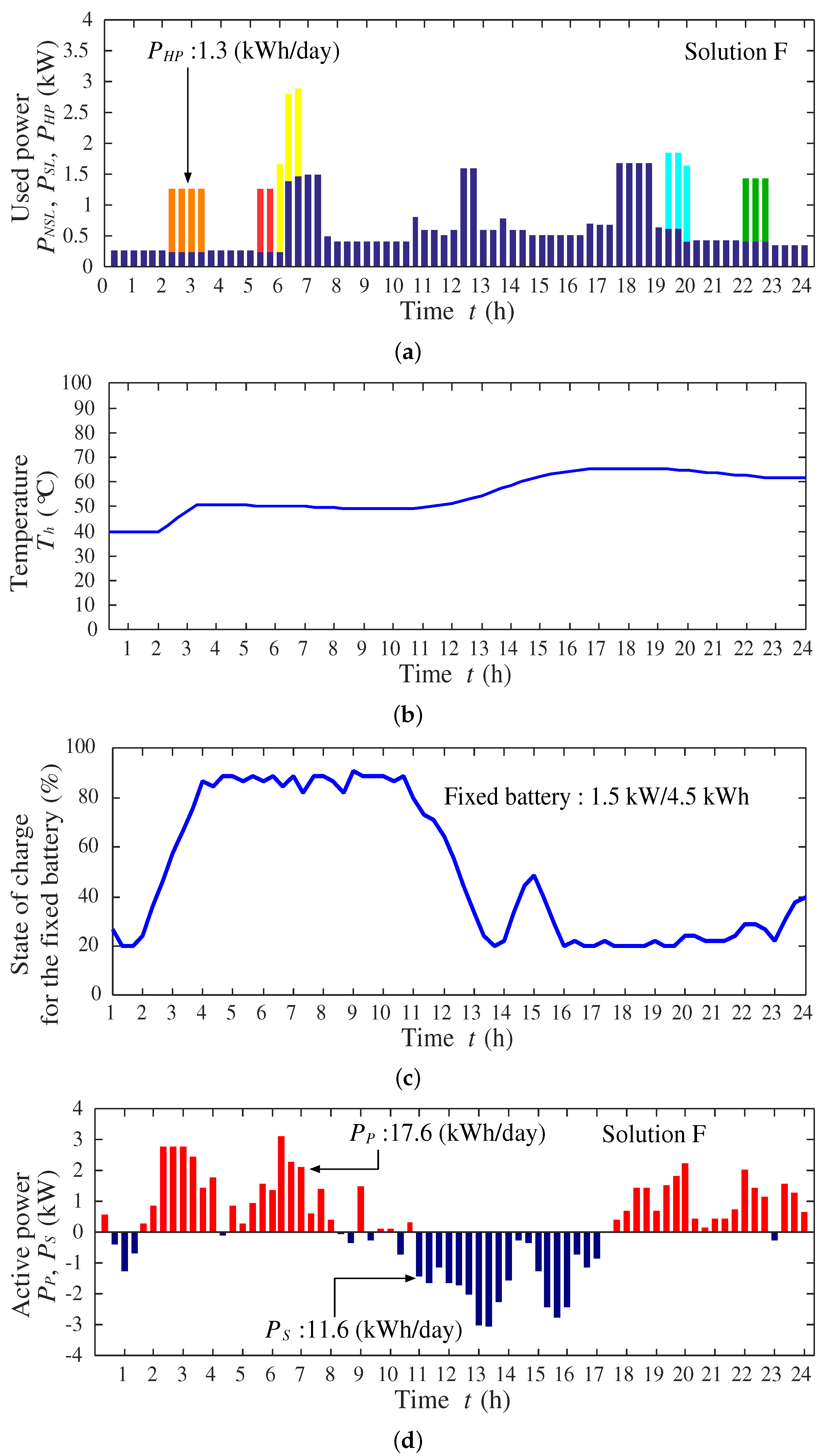
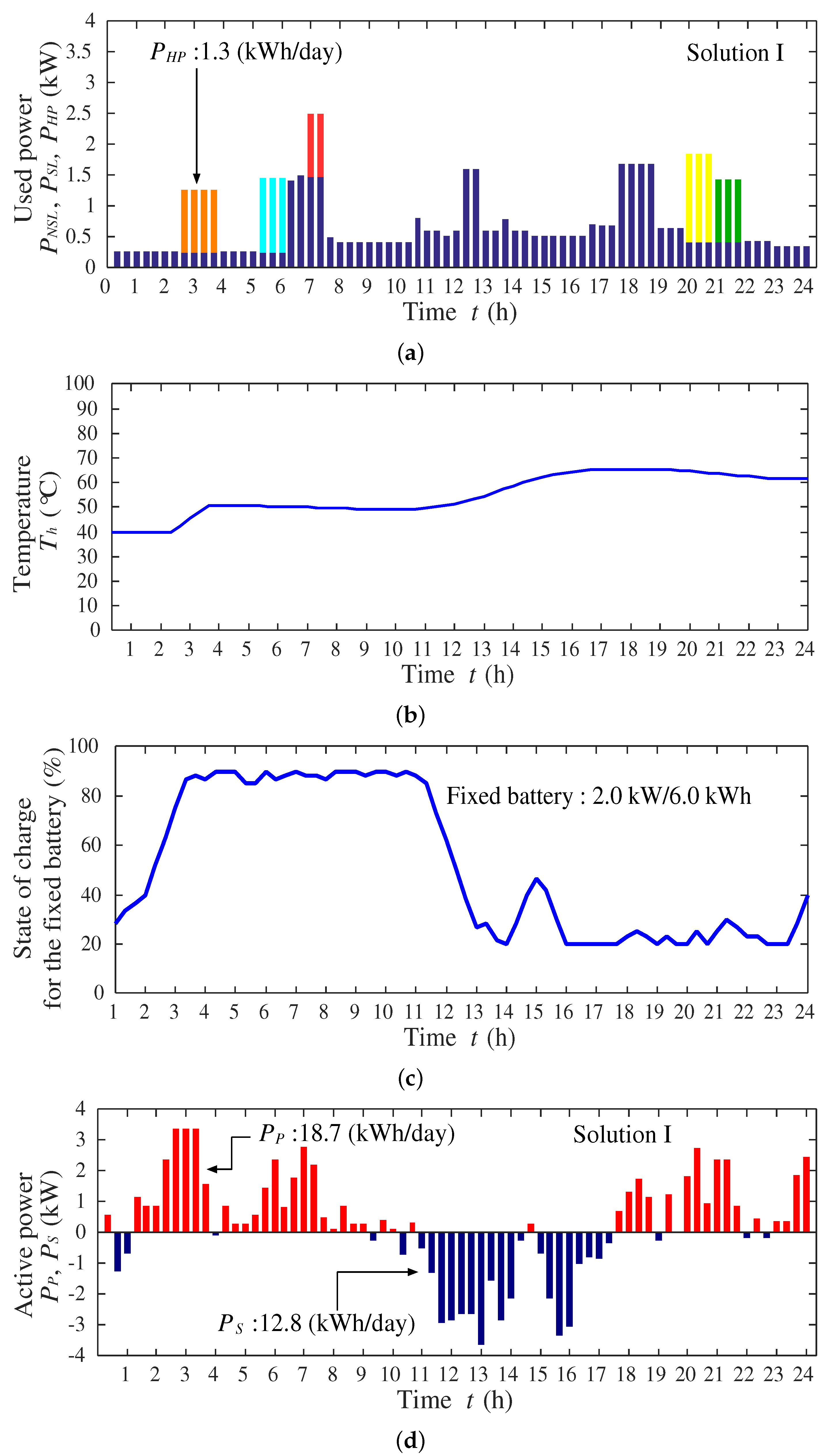
4.2. Discussion of the Simulation Results

The Pareto optimal front in each case obtained by the simulation is illustrated in Figure 11, and a comparison of the solutions is shown in

Table 2. Evaluation the result of the solutions.

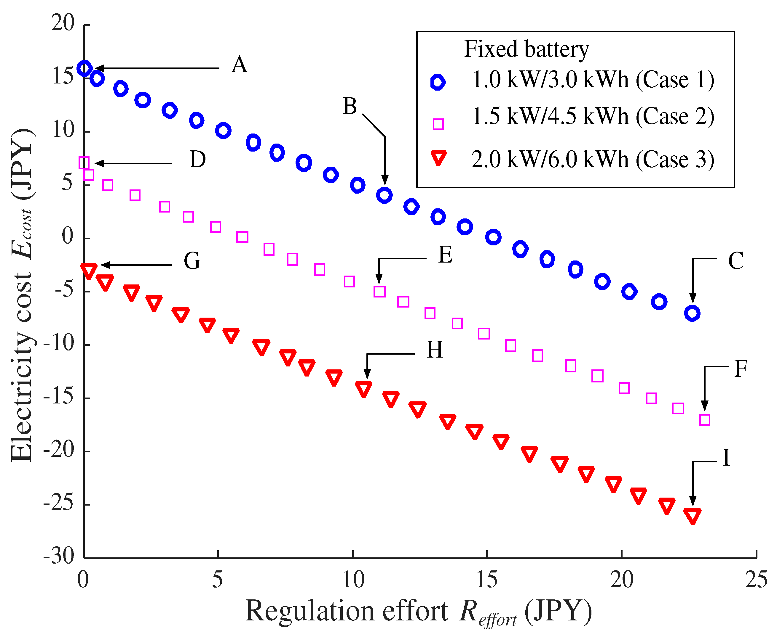
Case	Case 1			Case 2			Case 3
Solution	A	B	C	D	E	F	G	H	I
Regulation effort $R_{effort}$ (Yen)	0	11.2	22.6	0	11	23.1	0.2	10.4	22.6
Electricity cost $E_{cost}$ (Yen)	16	4.0	−7.0	7.0	−5.0	−17	−3.0	−14	−26

. From Figure 11 and Table 2, the relationship between regulation effort and electricity cost has a trade-off, and it is found that a large regulation effort reduces the electricity cost. Furthermore, it can be confirmed that a large capacity of the fixed battery reduces the electricity cost and regulation effort more. Therefore, if the resident in the smart house has a large capacity of the fixed battery, it is possible that a small regulation effort reduces the electricity cost.

The results of the solution in Cases 1, 2 and 3 in Figure 11 and Table 2 are each illustrated in Figure 12, Figure 13 and Figure 14, Figure 15, Figure 16 and Figure 17 and Figure 18, Figure 19 and Figure 20. In these figures, (a) is the modified use plan of the appliance and power consumption of HP; (b) is the temperature of hot water in the storage tank; (c) is the state of charge of the fixed battery; and (d) is the purchased and sold power. When comparing (a) of the same case, it can be confirmed that a large regulation effort reduces the power consumption of the appliance at the peak time. Furthermore, when comparing the use plan in a nearly equal regulation effort in the three cases, it is found that the use plan of the appliance is different. This is due to the changed use plan regardless of the type of appliance. Moreover, in the modified use plan of the appliance, since there is constraint Equation (21), use plan is not for the same time. Therefore, it is possible to perform a high feasibility regulation effort. From (b) in all cases, it can be confirmed that the target temperatures are satisfied at 7 a.m. and 8 p.m. by heating SC and HP. For (c) in all cases, the fixed battery is charged in the time zone of the low RTP price and is discharged in the time zone of the high RTP price. Therefore, it can be confirmed that the purchased power and electricity cost are reduced in the high RTP price. Comparing (d) in the same cases, a large regulation effort increases the purchased power in the low RTP price time zone and the sold power in the high RTP price time zone. Therefore, it can be confirmed that the electricity cost is reduced. Furthermore, comparing the solution in all cases, since a large capacity of the fixed battery increases the purchased and sold power, the electricity cost is reduced. Therefore, in a small regulation effort, the electricity cost is reduced by using a large capacity of the fixed battery.

5. Conclusions

In this research, the multi-objective optimization of a smart house applying the RTP system was proposed. The assumed smart house has PV, SC and, in addition, a fixed battery and HP as the controllable load. Consumers in the smart house plan the usage of the appliances depending on the RTP price. Reduced electricity cost is evaluated as the regulation effort. In [20], inconvenience, such as the time shift, is not generalized, but it can be indexed as the electricity cost by using the regulation effort. Optimal operation to minimize the regulation effort and the electricity cost was planned using the multi-objective optimization method. Moreover, the Pareto optimal fronts obtained in the simulation for different capacities of the fixed battery were compared. From the results of the simulation, it was indicated that it was possible to make an optimal operation plan that gives priority to the regulation effort or the electricity cost. Moreover, a consumer with a large capacity of the fixed battery reduces the electricity cost by a small regulation effort. Furthermore, it was indicated that a consumer with a small capacity of the fixed battery reduces the electricity cost by a large regulation effort.

References

- Organization for Cross-Regional Coordination of Transmission Operators (OCCTO), Tokyo, JAPAN. 2015. Available online: https://www.occto.or.jp/ (accessed on 31 March 2016).
- Ministry of Economy, Trade and Industry (METI), Tokyo, Japan. Retailers_List. Available online: http://www.enecho.meti.go.jp/category/electricity_and_gas/electric/summary/operators_list/ (accessed on 31 March 2016).
- Depuru, S.S.S.R.; Wang, L.; Devabhaktuni, V. Smart meters for power grid: Challenges, issues, advantages and status. Renew. Sustain. Energy Rev. 2011, 15, 2736–2742. [Google Scholar] [CrossRef]
- Santoshkumar; Udaykumar, R.Y. Development of Markov Chain-Based Queuing Model and Wireless Infrastructure for EV to Smart Meter Communication in V2G. Int. J. Emerg. Electr. Power Syst. 2015, 16, 153–163. [Google Scholar]
- Anees, A.; Chen, Y.P. True real time pricing and combined power scheduling of electric appliances in residential energy management system. Appl. Energy 2016, 165, 592–600. [Google Scholar] [CrossRef]
- Power Smart Pricing, Illinois, Ameren. Available online: http://www.powersmartpricing.org/ (accessed on 31 March 2016).
- Hattori, T.; Toda, N. Demand Response Programs for Residential Customers in the United States -Evaluation of the Pilot Programs and the Issues in Practice-. Available online: http://criepi.denken.or.jp/jp/kenkikaku/report/detail/Y10005.html (accessed on 31 March 2016).
- Midcontinent Independent System Operator. Available online: https://www.misoenergy.org/Pages/Home.aspx (accessed on 31 March 2016).
- Japan Center for Climate Change Actions (JCCCA). Available online: http://www.jccca.org/trend_world/conference_report/cop21/2-1212.html (accessed on 31 March 2016).
- Bracale, A.; Carpinelli, G.; Fazio, D.A.; Khormali, S. Advanced, Cost-Based Indices for Forecasting the Generation of Photovoltaic Power. Int. J. Emerg. Electr. Power Syst., 2014, 15, 77–91. [Google Scholar] [CrossRef]
- Central Research Institute of Electric Power Industry. Electric Power Condition in the World, Lessons for Japan. Available online: http://criepi.denken.or.jp/jp/serc/denki/world_book/eneco.pdf (accessed on 31 March 2016).
- Khederzadeh, M.; Khalili, M. High Penetration of Electrical Vehicles in Microgrids: Threats and Opportunities. Int. J. Emerg. Electr. Power Syst. 2014, 15, 457–469. [Google Scholar] [CrossRef]
- Reddy, S.S.; Abhyankar, A.R.; Bijwe, P.R. Co-optimization of Energy and Demand-Side Reserves in Day-Ahead Electricity Markets. J. Emerg. Electr. Power Syst. 2015, 16, 195–206. [Google Scholar]
- Nguyen, M.Y.; Nguyen, D.M. A Generalized Formulation of Demand Response under Market Environments. J. Emerg. Electr. Power Syst. 2015, 16, 217–224. [Google Scholar] [CrossRef]
- Tanaka, K.; Yoza, A.; Ogimi, K.; Yona, A.; Senjyu, T. Optimal operation of DC smart house system by controllable loads based on smart grid topology. Renew. Energy 2012, 39, 132–139. [Google Scholar] [CrossRef]
- Li, X.H.; Hong, S.H. User-expected price-based demand response algorithm for a home-to-grid system. Energy 2014, 64, 437–449. [Google Scholar] [CrossRef]
- Erdinc, O. Economic impacts of small-scale own generating and storage units, and electric vehicles under different demand response strategies for smart households. Appl. Energy 2014, 126, 142–150. [Google Scholar] [CrossRef]
- Rastegar, M.; Fotuhi-Firuzabad, M. Load management in a residential energy hub with renewable distributed energy resources. Energy Build. 2015, 107, 234–242. [Google Scholar] [CrossRef]
- Xia, S.; Ge, X. The Optimized Operation of Gas Turbine Combined Heat and Power Units Oriented for the Grid-Connected Control. J. Emerg. Electr. Power Syst. 2016, 17, 143–150. [Google Scholar] [CrossRef]
- Soares, A.; Antunes, C.H.; Oliveira, C.; Gomes, L.A. multi-objective genetic approach to domestic load scheduling in an energy management system. Energy 2014, 77, 144–152. [Google Scholar] [CrossRef]
- Xu, S.; Yan, Z.; Zhao, X.; Zhang, L.; Feng, D.; Xu, X. Decentralized Charging of Plug-In Electric Vehicles Using Lagrange Relaxation Method at the Residential Transformer Level. J. Emerg. Electr. Power Syst. 2016, 17, 267–276. [Google Scholar] [CrossRef]
- Yoza, A.; Yona, A.; Senjyu, T.; Funabashi, T. Optimal capacity and expansion planning methodology of PV and battery in smart house. Renew. Energy 2014, 69, 25–33. [Google Scholar] [CrossRef]
- Shimoji, T.; Tahara, H.; Matayoshi, H.; Yona, A.; Senjyu, T. Comparison and Validation of Operational Cost in Smart Houses with the Introduction of a Heat Pump or a Gas Engine. J. Emerg. Electr. Power Syst. 2015, 16, 59–74. [Google Scholar] [CrossRef]
- Yoza, A.; Uchida, K.; Yona, A.; Senju, T. Optimal Operation Method of Smart House by Controllable Loads based on Smart Grid Topology. J. Emerg. Electr. Power Syst. 2013, 14, 411–420. [Google Scholar] [CrossRef]
- Shimoji, T.; Tahara, H.; Matayoshi, H.; Yona, A.; Senjyu, T. Optimal Scheduling Method of Controllable Loads in DC Smart Apartment Building. J. Emerg. Electr. Power Syst. 2015, 16, 579–589. [Google Scholar] [CrossRef]
- Uchida, K.; Senjyu, T.; Urasaki, M.; Yona, A. Installation Effect by Solar Pool System Using Solar Insolation Forecasting. In Proceedings of the 2009 Annual Conference of Power & Energy Society, Seoul, Korea, 26–30 October 2009; Volume 25, pp. 7–12.
- Shadmand, M.B.; Balog, R.S. Multi-Objective Optimization and Design of Photovoltaic-Wind Hybrid System for Community Smart DC Microgrid. IEEE Trans. Smart Grid 2014, 5, 2635–2643. [Google Scholar] [CrossRef]
- Ghazvini, M.A.F.; Soares, J.; Horta, N.; Neves, R.; Castro, R.; Vale, Z. A multi-objective model for scheduling of short-term incentive-based demand response programs offered by electricity retailers. Appl. Energy 2015, 151, 102–118. [Google Scholar] [CrossRef]
- Kamjoo, A.; Maheri, A.; Dizqah, A.M.; Putrus, G.A. Multi-objective design under uncertainties of hybrid renewable energy system using NSGA-II and chance constrained programming. Int. J. Electr. Power Energy Syst. 2016, 74, 187–194. [Google Scholar] [CrossRef]
- Deb, K.; Pratap, A.; Agarwal, S.; Meyarivan, T. A fast and elitist multiobjective genetic algorithm: NSGA-II. IEEE Trans. Evol. Comput. 2002, 6, 182–197. [Google Scholar] [CrossRef]