1. Introduction
Wastewater treatment plants (WWTPs) play a fundamental role in the water supply chain as they enable water sanitation and reuse. Wastewater treatment is the process where organic and inorganic pollutants are removed from the sewage. Wastewater cannot be released directly into the environment as soil, sea, rivers, and lakes are unable to degrade quantities of polluting substances higher than their own disposal capacity. The main pollutants that can be removed following treatment are biodegradable organics (e.g., biochemical oxygen demand (BOD)), suspended solids, nitrates, phosphates, and pathogenic bacteria. With the current emphasis on environmental health and water scarcity affecting some European countries, there is a growing awareness of the need to dispose of such wastes in a safe and beneficial way, as instructed by the Directive 91/271/EU [
1] on urban wastewater treatment, and Directive 2013/39/EU [
2] on monitoring micro-pollutants.
Two main challenges characterize the industry: increasing the environmental sustainability of the treatment process and minimizing the economic cost for operating the service. The expenditure on wastewater management and treatment in the European Union with 28 member states was around 0.60% of GDP in 2011 [
3].
In order to achieve these strategic objectives, water utilities might adopt different policies. Scientific literature often suggests the renewal of the whole plant or a part of it, introducing devices for energy recovery [
4,
5], or for raw material recovery from sludge [
6], or high tech solutions that improve the efficiency of reagent dispensing and consumption. Innovations have been continually developed for wastewater and sludge treatments [
7,
8]. Additionally, some interesting innovations were also developed in relation to materials such as coagulators and flocculants used to facilitate the treatment process, which resulted in increased removal rates of pollutants and lower sludge volume indices [
9,
10].
However, to the best of our knowledge, there is no evidence of a Performance Measurement System (PMS) based on a set of key performance indicators (KPIs), financial and non-financial, that aids the management of water utilities. A PMS includes measures to evaluate the efficiency and effectiveness of a manager’s actions and acts as a control process [
11]. A correctly designed PMS ensures improvement in achieving the firm’s strategic objectives. The PMS framework, which represents an evolution of management control systems (MCS), integrates strategy goals and KPIs, as well as financial, quality, and technical measures [
11].
Literature on performance measurement in WWTPs is based only on technical indicators [
12,
13]. Only recently have some scholars proposed an integration of technical, economic, and environmental performance in a single indicator [
14,
15]. The previously proposed framework integrating financial and non-financial measures had regulatory purposes [
16] or alternatively was aimed at identifying short and long term drivers of plants’ performance [
17,
18]. However, there is lack of work on a PMS developed to improve efficiency and profitability of WWTPs from an internal and managerial perspective, with a process of plan-do-check-act. Recently, some interesting models where developed, but they followed only an ex ante approach, based on simulation and on benchmarking scenarios [
19].
The current paper develops a PMS with a set of KPIs linked by cause and effect relationships, based on the Balanced Scorecard model [
20,
21]. This tool was tested on a wastewater utility covering more than 1 million population equivalent (PE) and located in Italy. The tool was used to assess its effectiveness in helping the management to identify key factors affecting the plant’s performance. During the study, 17 KPIs grouped in four different clusters were measured for three years. Structural Equation Modeling (SEM) was used to identify the cause and effect linkages among the KPIs.
The research addresses the literature gap on performance measurements of WWTPs, launching an integrated reporting tool and providing a managerial approach to this issue, based on several types of measures linked by causal linkages. The novelty of the article is that it provides to water utilities a tool which supports the management in finding activities with poor performance, designing a strategic map among KPIs, and allowing them to delay non-relevant measures of control.
The remainder of the paper is structured as follows. The next section provides a description of the case study, which is one of the largest plants in Tuscany; the third section discusses the PMS, selection of KPIs, and describes the statistical analysis for identifying the main drivers of performance. The fourth section describes the results obtained following the adoption of the PMS in the wastewater utility and discusses their practical implications.
2. Main Characteristics of the Case Study
The study was conducted at the Baciacavallo site of Gestione Impianti Depurazione Acque (GIDA), which means Management of Wastewater Treatment Plants. The utility was founded in 1981 on the basis of the Italian National Law 319/1976 [
22] that requires more sustainable practices in water management. GIDA is a public-private company with three partners: Prato Town Council (with 46.5% of shares), Confindustria (an Industrial Association with 45.5% of shares), while the remaining 8% is owned by a company wholly controlled by the municipalities in the area.
The WWTP at Baciacavallo is composed of two water lines constructed at different times: 1980 and 1986. Wastewater collected from an old sewerage for domestic customers and two industrial districts is treated here. In 2001, a new hydraulic connection was established with the WWTP of Calice, also owned by GIDA.
The plant of Baciacavallo was designed to treat 130,000 m3/d of sewage, with a daily average input load of 220 mg/L of chemical oxygen demand (COD) and 200 mg/L of biochemical oxygen demand (BOD5). The design capacity of the plant, calculated on the basis of the available water supply of 0.2 m3/PE, corresponds to 650,000 PE.
Wastewater effluent from the sewerage is subject to mechanical treatment using desanders and primary sedimentation and is, thereafter, stored in two equalization tanks. Then, the wastewater is transferred to biological basins for nitrification and oxidation. Subsequently, the wastewater is subjected to secondary sedimentation, tertiary treatment, ozonation, and finally discharged into the Ombrone River. The sludge that is produced during the treatment of sewage is thickened, dewatered by centrifugation, and then incinerated.
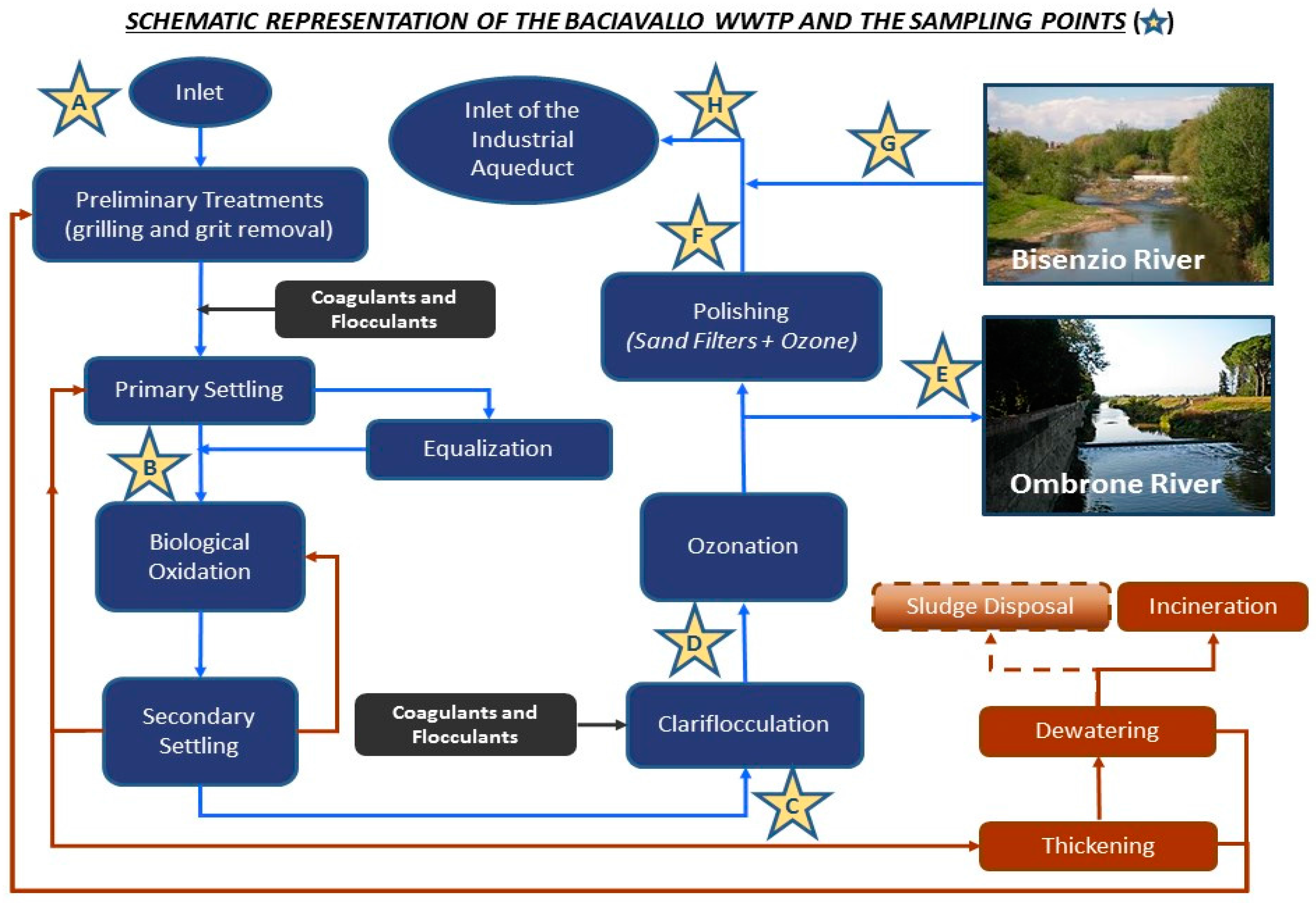
Figure 1 shows the structure of the plant.
2.1. Primary Treatment
Wastewater from the sewerage collector is treated using two vertical grids. Thereafter, it is raised by four Archimedes screw pumps and sent for fine screening. The solid material is collected in a container and disposed of as waste, while wastewater is collected by the drainage system which discharges into the head of the plant.
The residues present in the liquid phase are separated from the wastewater using two vertical fine grids. After fine filtration, the flow of wastewater is divided into two treatment lines that cross through four circular tanks, called desanders, each with a volume of 50 m3. The solid waste obtained is collected in a container and disposed of as waste in a similar manner to that described for the first step of gridding.
The core of the primary treatment consists of four tanks of 10,800 m3 with a slow mixing mechanism where the sewage is exposed to ferric chloride and anionic polymer and five rectangular tanks where the settling of solids takes place. The settled sludge is periodically extracted and transferred to the thickening tanks of the sludge line. Each line is equipped with a rotating grid for filtering and separating floating solids extracted from the primary sedimentation.
The wastewater from the primary treatment is stored in two circular tanks of 11,000 m3 each, which serve as equalization basins. Subsequently, wastewater is sent to oxidation tanks for biological treatment using Archimedes screw pumps that raise the water at 1500 m3/h.
2.2. Secondary Treatment
The effluent from the primary sedimentation, or that raised from the equalization tanks, is sent to four oxidation/nitrification tanks, with a capacity of 7500 m3 each, equipped with superficial rotors that provide the air required for the oxidation process.
Following nitrification, the wastewater is sent to four circular sedimentation tanks with volumes of 7654 m3 each, equipped with mechanically driven scrapers that continually drive the collected sludge towards a hopper in the base of the tank where it is pumped to sludge treatment facilities, or recycled to the same oxidation tank to increase the sludge retention time (SRT).
In particular, the extracted sludge from the sedimentation can follow two different paths:
- ➢
Resent to the oxidation tanks to keep the concentration of biomass constant, through four recirculation screws with speeds of 2160 m3/h each;
- ➢
Sent to thickening tanks through four pumps.
2.3. Tertiary Treatment
Following oxidation/nitrification, wastewater flows in tanks equipped with electric mixers, where aluminum trichloride (TRIAL) and anionic polyelectrolyte are added. Subsequently, wastewater is sent for final sedimentation. The sludge produced in this phase is collected and sent at 40 m3/h using extraction pumps to the thickening process of the sludge line.
2.4. Ozonation
The wastewater from the tertiary treatment is sent through a pipe to a pumping station, and then sent to contact tanks for ozonation. The scope of the ozone treatment is to reduce the color and the concentration of surfactants, which have not been degraded by the biological-oxidative process. Ozone is generated by means of four ozonators working with pure oxygen.
Ozone gas is produced from liquid oxygen stored in four tanks. Ozone generators produce gas by passing electrical discharges of high intensity through oxygen gas. The process yields about 10% (kg of ozone [O3] per kg of oxygen [O2]). The gas mixture produced is blown through a network of porous disks in three basins of contact consisting of four compartments, which contain the wastewater after the tertiary treatment. The maximum capacity of ozone generation is 200 kg/h (50 kg per generator), and the power of each is approximately 350 kW.
2.5. Sludge Treatment
The excess sludge from the tertiary and secondary treatments is sent to a thickener, with a capacity of 900 m3, and subsequently to two other thickeners of similar volumes, where the extracted sludge from the primary sedimentation also converges. Sludge originating from the plant at Calice is transported through a dedicated pipe called “fangodotto” and is also processed here.
The thickened sludge is then dewatered through two centrifuges with capacities of 45 m3/h after the addition of cationic polyelectrolyte. The dehydrated sludge is pumped in two storage silos, with capacities of about 75 m3 each, and sent to the incinerator through pumps.
3. Performance Measurement System for WWTPs
The PMS developed for the case study was quite similar to the balanced scorecard of Kaplan and Norton (1992), as it is also structured in four perspectives. However, the financial, customer, process, and knowledge areas of the well-known reporting tool were replaced by other parameters more suited for WWTPs, such as costs, quality, efficiency, and external environment (
Figure 2). The PMS was developed in collaboration with GIDA, following the framework of Istituto Superiore per la Protezione e la Ricerca Ambientale (ISPRA) [
23].
In total, 17 KPIs were identified. Five were related to the cost perspective and referred to direct and variable cost items. They included energy, reagents, and sludge disposal costs per cubic meter. Any positive (or negative) variation of costs measured by the report can be interpreted as a loss (or gain) of economic efficiency.
Other costs, even if relevant, were excluded from this analysis, as they do not vary with the volume of wastewater treated or its pollutant load, such as staff, maintenance costs, amortization, and depreciation of assets. Staff is among the first three cost items of WWTPs, with energy and sludge disposal. However, different from these last items, staff is strictly fixed, and its variation in the short term might not depend on the plant’s workload. The cost KPIs where chosen according to the plant’s characteristics. Energy costs included: (1) costs for the classic treatment for wastewater and sludge (ucENcla), including grid, primary sedimentation, active sludge, secondary sedimentation, sludge dewatering, and drying; (2) costs for the ozone treatment for the removal of color and surfactants (ucENoz). Similarly, reagents costs for the wastewater treatment (ucREAGwa) were included, such as aluminum trichloride, anionic polyelectrolyte, and oxygen consumed, and for the sludge treatment (ucREAGsl), where cationic polyelectrolyte was added to facilitate flocculation and sedimentation of the suspended solids; and, finally; (3) disposal costs (ucDISP) measured for the expenditure of transporting the sludge to the landfill, composting plants, farms, or incinerators. The sludge treatment cycle’s output produced by Baciacavallo and Calice plants was fed into the incinerating process.
Costs were calculated in reference to the volume of wastewater treated (€/m
3). An alternative measure would be the unit cost per kg of pollutants removed (e.g., €/kg COD). Both measures have their own advantages and limits. The former quantifies pure cost efficiency, but is affected by the rate of storm water that mixes with the sewage. Actually, the cost per cubic meter usually decreases when this rate increases, consequently sewer networks with higher infiltrations could appear more efficient than others with equivalent volume. The latter relates to costs of the effective output of a WWTP, but could be affected by exogenous variables such as the COD concentration of the influent wastewater, which cannot be wholly controlled by the plant manager. The pollution concentration of the input wastewater has a negative effect on efficiency and removal rate, according to Fraquelli and Giandrone [
24] and Lorenzo-Toja et al. [
25]. This can explain the higher costs incurred to remove an intense pollutant load.
The quality perspective includes three KPIs measuring the removal rate of three pollutants: total suspended solids (SST), COD, and color. The suspended solids and the COD are two classic indices of pollution. Nitrogen (N) removal rate was not included to not burden the PMS, since the wastewater inflows of GIDA are characterized by the other pollutants mentioned and the amount of nitrate in the discharged effluent are considerably under the maximum limit provided by the environmental law.
The indicators were estimated using Equation (1):
where rCOD, rSST, and rCOL are the quality indexes for the removal of COD, SST, and color, respectively; RR
exp is the expected removal rate, estimated as the average removal rate recorded in the previous years; and RR
act is the actual removal rate measured in the current period.
This method of computation assigns a score that increases with higher removal rate. A similar score is estimated when technical efficiency is measured. The company decided to set a target on the basis of its past performance and not according to the standard set by the scientific literature. This choice could be explained considering that the literature usually provides standards for plant treating only domestic wastewater, while the Baciacavallo plant operates on non-domestic wastewater, coming mainly from textile industries, for which it is very difficult to find generally accepted performance standards in terms of quality and efficiency.
Energy and reagents consumption were split in two measures based on their consumption during the classic and ozone treatment phases. Sludge treatment was monitored using three indicators that referred to the volume of sludge produced, quality of treatment, and disposal.
The two energy efficiency measures (enCLA and enOZ) were quantified by the ratio of the expected kWh to the actual kWh consumed in the classic and ozone treatments. A growth (decrease) of the score identifies a savings (loss) of efficiency, as shown in Equation (2).
A similar measure was obtained for the reagents (Equation (3)). The efficiency of reagents for ozone (reagOZ) is the ratio of the expected to actual amount of oxygen consumed.
For the classic treatment (reagCLA), the global score of efficiency in terms of reagent consumption was calculated using a weighted average of the scores estimated for the three types of chemicals used (anionic and cationic polyelectrolyte and aluminum trichloride). The weights specified in Equation (4) were chosen by the management of GIDA, considering their relative importance in the process of the treatment.
The production of sludge (slPROD) for the Baciacavallo plant was measured by the ratio of the expected weight of SST to the actual volumes. This indicator was not directly handled by the plant managers as it mainly depends on the SST concentration in the wastewater inflow. However, its measurement is crucial as the total amount of SST can affect the disposal costs indicator included in the economic perspective.
The efficiency of treatment (slTREAT) quantifies the capability of the plant to reduce the amount of organic suspended solids in the stabilized sludge and its humidity, as shown in Equation (5):
where SSV is the percentage of the volatile solid (organic) included in the sludge and DM is the percentage of dry matter obtained.
The sludge treatment efficiency was obtained using both ratios with two weights chosen by the management of GIDA.
The last technical efficiency indicator was sludge disposal (slDISP) that measures the amount of energy and raw material recovered, and was estimated using Equation (6):
KPIs pertaining to the plant performance included two indicators related to wastewater characteristics: COD concentration of sewage inflow (CODcon) measured in terms of mg/L, and volume of inflow (VOLinf), measured in terms of cubic meters.
Plant performance on the basis of the 17 KPIs was collected monthly for three years, from 2013 to 2015. In total, 612 observations were collected and SEM approach was applied to identify the cause and effect relationships among the KPIs and to identify effective performance drivers for the plant studied.
The KPIs observed could be linked following several combinations.
Linkages among KPIs can be non-sequential as a component of one balanced scorecard perspective has a cause and effect relationship with one or more components of other perspectives and not necessarily with those included in the level immediately above, as in the case of “sequential” linkages [
26,
27,
28]. Furthermore, interdependent linkages arise when two KPIs of different levels have a bidirectional relationship, also called a “reverse linkage” [
29]. Finally, two KPIs of the same perspective can exhibit an intra-dependent relationship. All these links could be indirect or direct, and may involve other KPIs as mediators.
SEM is one of the best approaches to map all these nexuses [
29,
30]. SEM adopts different mathematical models to study relationships among variables and it often studies latent variables, which are not directly observed, but only inferred from other measures (e.g., the quality of life can be measured inferring wealth or environment). Path analysis is a special application of SEM, applied only to observed variables [
31]. Path analysis is based on a set of multivariate regression functions. The method is suited to identify direct and indirect effects of causal variables. Path analysis has already been used to draw the causal relationships among KPIs [
32,
33,
34,
35]. SEM using path analysis was applied in this study.
Considering the 17 KPIs as a non-oriented network [
36], the potential causal relationships are identified as
, where n represents the number of nodes of the network. In our study, there could be
connections. To avoid a complex system of multivariate regression functions, a correlation matrix was built to identify all significant nexuses among KPIs, excluding those that are not relevant.
Thereafter, each KPI was related to its potential drivers and mapped with the correlation matrix. A variety of estimation methods have been used in SEM, however, three standard methods that almost all SEM programs support are ordinary least square (OLS), generalized least square (GLS), and modified least square (MLS).
The current research is based on OLS and applies a post estimation assessment using the F-test. Unlike
t-tests that can assess only one regression coefficient, the F-test can assess multiple coefficients simultaneously. The F-test compares a model with no predictors to a specified model [
37]. While R-squared values estimate the strength of the relationship between dependent and independent variables, the F-test determines whether this relationship is statistically significant; if the
p-value for the test is lower than a certain threshold the R-squared value is statistically significant.
F is measured as the ratio between the explained and unexplained variance of the dependent variable, as summarized by Equation (7).
where SSR is the sum of square regression, SSE is the sum of square error, df is a degree of freedom, and MSR and MSE are the mean sum of square due to treatment and error, respectively.
The ratio indicates when the independent variables do not exert any significant impact on y. This null hypothesis must be accepted when the p-value of the test is under a threshold (usually 5%).
4. Results of PMS Implementation
An overview of the data collected for the plant at Baciacavallo is reported in
Table 1. All the KPIs in the quality perspective were greater than 1, which demonstrates that GIDA was performing well in the quality perspective. However, a wide variation was recorded for the SST removal rate, as shown by the relative standard deviation index. Among the KPIs pertaining to technical efficiency, only reagent consumption was greater than 1, while energy and sludge performance decreased from 2013 to 2015. A wide variation was recorded for reagent consumption, sludge production, and energy consumed for the ozone treatment. Furthermore, the energy consumption in classic treatment, sludge treatment, and disposal was relatively stable. Exogenous variables observed included approximately 3 mil of m
3 treated monthly with an average COD concentration of 218 mg/L. Both these variables varied during the three years, as the relative standard deviations were 15% and 21%, respectively. The cost observed had a total value of 1.08 €/m
3, obtained by adding the mean values reported in
Table 1. In order of relevance, the main costs were for energy in classic treatment, sludge disposal, and energy in ozone treatment. The cost for reagents in water treatment was about 21% of the energy costs, while the cost for reagents in the sludge treatment was about 6% of energy costs.
Before the path analysis, a correlation matrix was drafted to identify variables linked by potential cause and effect nexus (see
Table 2). This tool was applied to choose the dependent variables of the regression functions estimated during the path analysis. According to the method applied, variables included in the statistic models must show a Bravais Pearson correlation index greater than 0.20.
Considering that exogenous variables are affected by environmental factors not measured by the PMS, and disposal costs do not have any relevant correlation index, this paper studied 14 regression functions structures, as reported in
Table 3, with R
2, adjusted R
2, and
p value of the F-test. We observed that R
2 was between 0.20 and 0.66. The
p value of F-test was always under 0.05; therefore, the null hypothesis of the test, which specified that the independent variables do not exert any effect on y, had to be rejected.
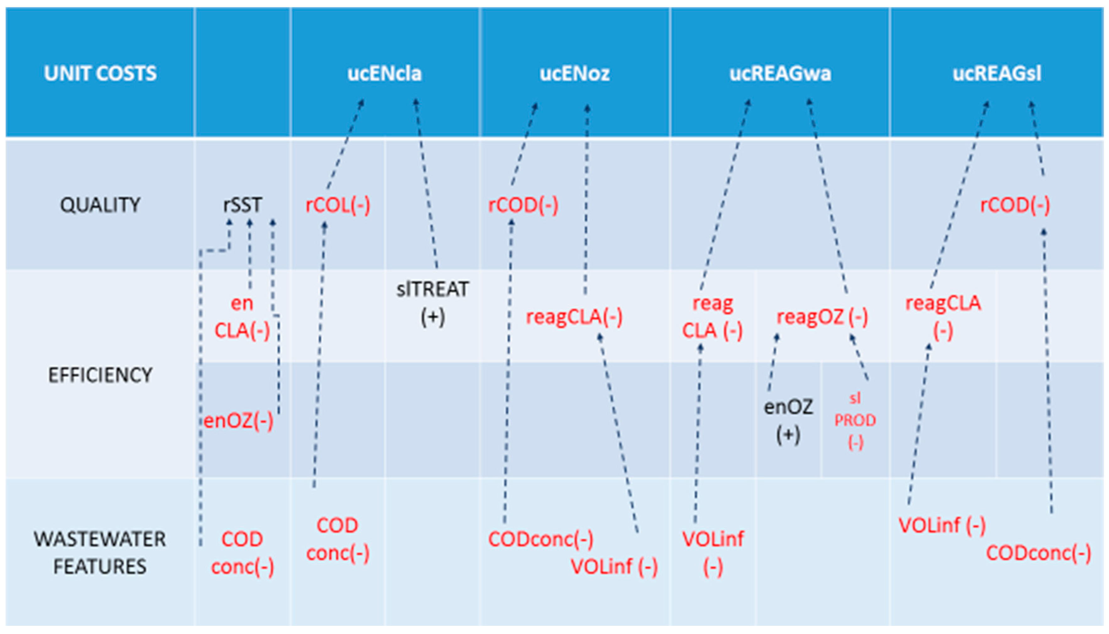
Figure 3 summarizes the key findings of the path analysis. The algebraic sign near each measure indicates the effect exerted on the related KPI: “+” is positive and implies a directly proportional correlation, while “−” is negative and implies an indirectly proportional relationship.
Unit costs were directly affected by the removal rate of pollutants (COD and color), with the exception of ucREAGwa. All unit cost indicators were directly affected by at least one KPI of technical efficiency; and, furthermore, they were always conditioned indirectly by exogenous variables.
VOLinf and CODcon played relevant roles in the PMS designed in this research. The pollutant load affects the quality perspective, affecting the SST, COD, and color removal rate; simultaneously, the COD concentration had an effect on the cost, mediated by the COD and color removal rate. Therefore, a high concentration of pollutant load in the wastewater inflow results in a decrease in the removal rate of COD and color, and (indirectly) an increase in costs (with the exception of reagents added to the water treatment). This highlights that a higher pollutant load, measured in terms of carbon and color, requires more intense work by the plant, but achieves poorer results in terms of quality.
The Bravais Pearson correlation coefficients reported in
Table 2 demonstrate that an increasing pollutant load required higher energy consumption in classic and ozone treatments, and higher consumption of reagents in the classic treatment. Furthermore, energy is required to achieve a higher removal rate in terms of suspended solids.
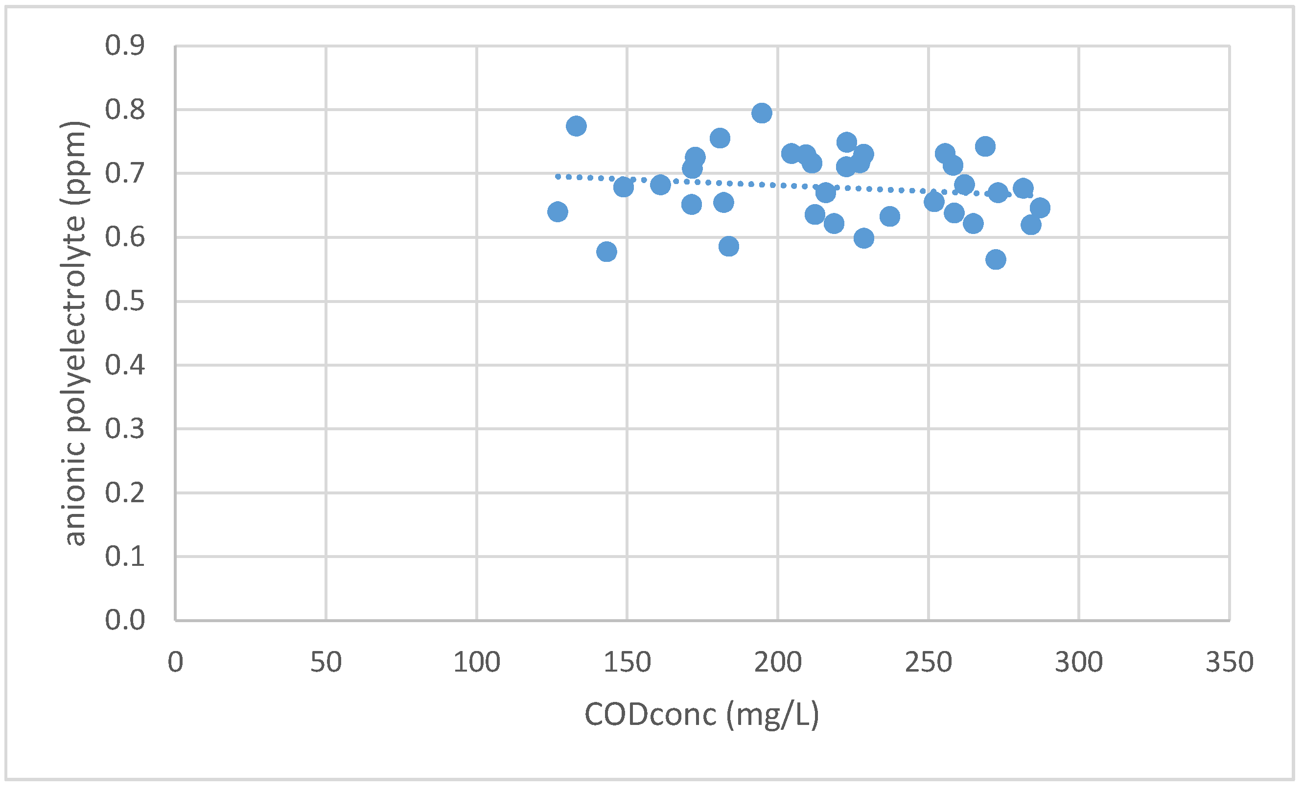
The relationship between each type of chemical added and CODcon was studied to understand the trend in consumption of reagents.
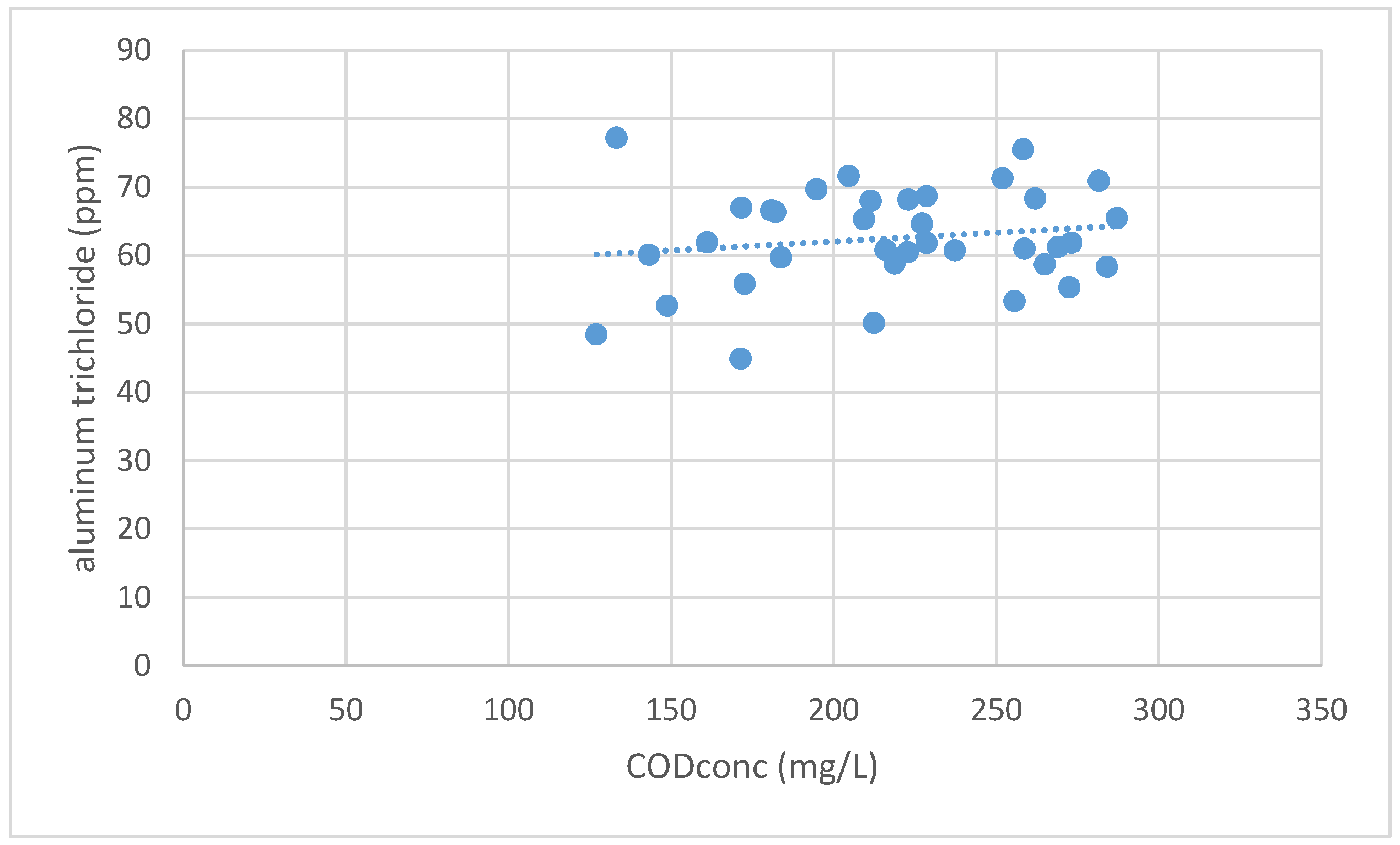
Figure 4 and
Figure 5 show the consumption of reagents added during the water treatment, and
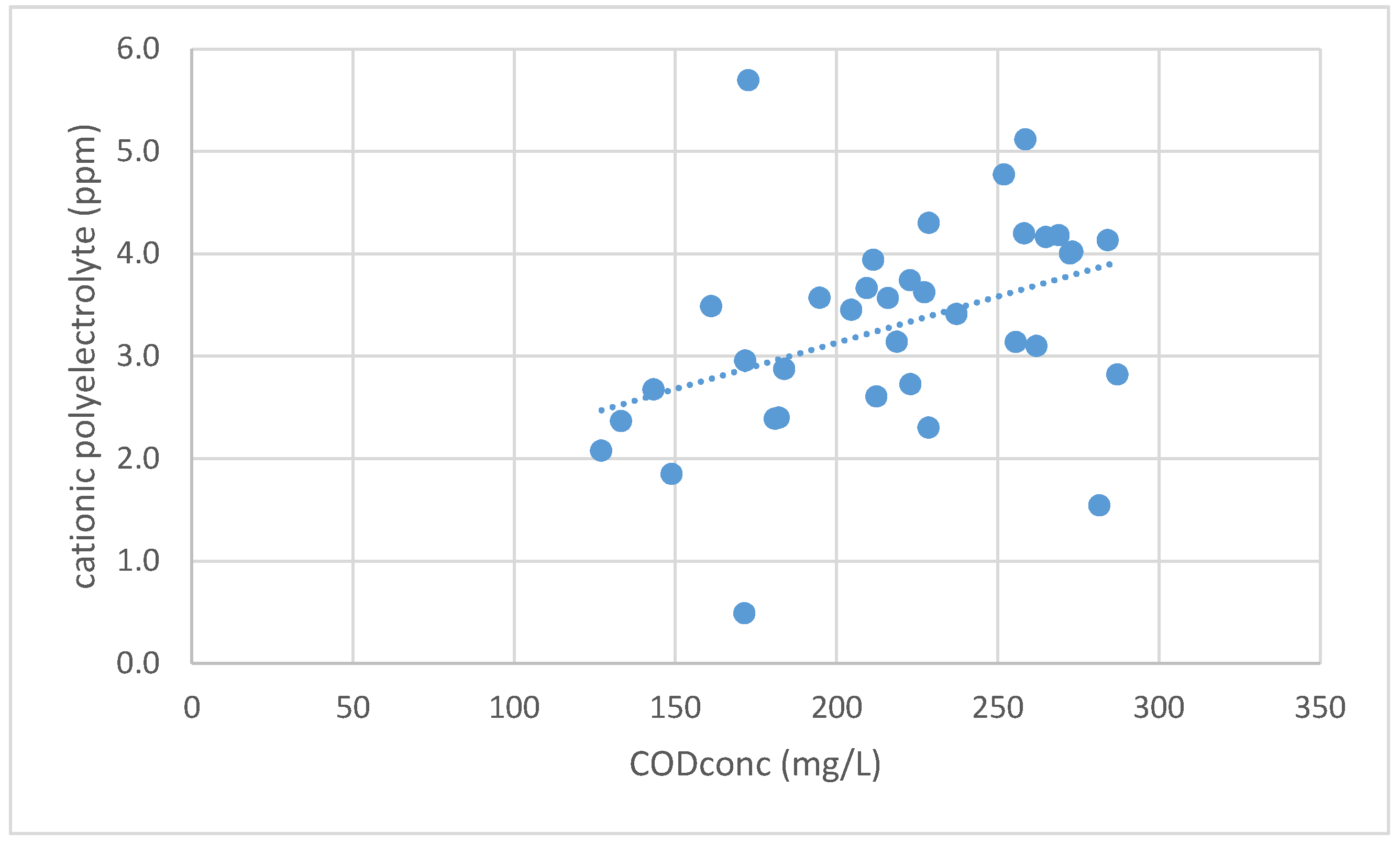
Figure 6 refers to the consumption of cationic polyelectrolyte during the sludge treatment. Only anionic polyelectrolyte (
Figure 5) was employed in larger amounts when the pollutant load decreased. In contrast, the amount of cationic polyelectrolyte and aluminum trichloride increased with heavier wastewater inflow. These results explain why ucREAGwa was not affected by CODcon; one of the two chemicals employed was not used following the pollutant load and counterbalanced the cost savings effected by the other reagent.
Therefore, an analysis of the variation in the volume of wastewater treated on reagents dosage was conducted. VOLinf influenced the quantity of reagents used in the classic treatment (water + sludge); a higher value of this exogenous variable determined a loss in efficiency of reagent consumption and an increase of reagents for water (ucREAGwa) and sludge treatment (ucREAGsl). This decreasing return to scale in reagent consumption and relative costs were due to some weakness of the dosage activity, as the ability of devices to vary the quantity of chemicals added on the basis of controlled factors, such as volume and pollutants concentration, is not properly developed.
These observations on reagents consumption were also confirmed by the analysis of cause and effect relationships on the technical efficiency perspective. Firstly, the measure of efficiency for consumption of reagents in the classic treatment affected all costs as shown in
Figure 3, with the exception of ucENcla. This means that this technical KPI should be analytically controlled by the plant manager of Baciacavallo. Secondly, the consumption of oxygen for the ozone treatment was affected by the quantity of sludge treated and produced; an increase (or decrease) in sludge production determined a decrease (or increase) in reagent consumed in the ozone treatment. This counterintuitive result could be explained in terms of the inefficiency that characterizes the dosage activity.
Among technical efficiency KPIs, energy measures play a relevant role as quality drivers and not as costs drivers (like reagOZ and reagCLA). Both types of measures for energy (classic and ozone) were crucial to achieve a good removal rate of SST as the treatment to remove solids properly from the wastewater needed a lot of energy for mechanical filtration, sand removal, and primary and secondary sedimentation. However, enCLA and enOZ do not affect energy costs as energy is a mixed cost that does not proportionally vary with kWh consumption and volume of wastewater treated; furthermore, the cost also varies with the price negotiated with the providers. In the period observed, the purchasing price per MWh decreased: GIDA paid an energy cost of 154.5 €/MWh in 2013, 155.2 €/MWh in 2014, and 145.5 €/MWh in 2015. At the same time, the enCLA indicator was 0.95 in 2013, 1.05 in 2014, and 0.92 in 2015. This confirms that GIDA took advantage of lower prices, and increased consumption in 2015; however, in terms of cause and effect relationship, the price variation counterbalanced the consumption variation, neutralizing its effects on unit costs.
Thus, the tool developed in this study provided wide support to GIDA’s staff in identifying the key performance drivers and their main effects that must be continuously monitored. The following conclusions can be drawn from this case study.
Quality is a perspective of performance that requires high energy consumption in both classic and ozone treatments; an improvement of the removal rates requires higher power consumption in the plant. Further, quality also depends on the pollutant load; with a low COD concentration, higher removal rates were achieved with lower costs per cubic meter. This highlights the benefits that could be obtained by the plant from a more diluted sewage, for example, during rainy weather. Costs are affected by quality, reagent consumption, and sludge treatment among the technical efficiency KPIs. A weakness of the treatment process was highlighted by the PMS, with reference to reagents. An increase in consumption did not generate any benefits to the removal rate, and increased costs. Additionally, the negative relationship between sludge produced and oxygen consumption can be considered as a warning. It means that oxygen in ozone treatment is consumed regardless of the SST to be removed, so that a rationalization of this activity is required, for example, dosing the ozone according to the pollutants load of the wastewater to be treated.
Finally, indirect linkages reveal that the volume of wastewater inflow and pollutant load affect the plant unit cost through their effects on quality and efficiency. An increase in volume damages technical efficiency and increases cost; while the removal of high pollutants concentration is hard and expensive. However, as demonstrated by prior literature [
38], the concentration of pollutants could exert an opposite effect when functional units different from volume are adopted as the COD is removed.
Thus, the study highlights the importance of a PMS that links technical measures, usually monitored by engineers and chemists, with costs and other financial measures, usually controlled by the chief financial officer of a water utility. The integrated reporting developed assists production managers in identifying the economic effects of their choices, while financial officers can understand the real causes of poor financial performance.


