Airline Sustainability Modeling: A New Framework with Application of Bayesian Structural Equation Modeling

Abstract

There are many factors which could influence the sustainability of airlines. The main purpose of this study is to introduce a framework for a financial sustainability index and model it based on structural equation modeling (SEM) with maximum likelihood and Bayesian predictors. The introduced framework includes economic performance, operational performance, cost performance, and financial performance. Based on both Bayesian SEM (Bayesian-SEM) and Classical SEM (Classical-SEM), it was found that economic performance with both operational performance and cost performance are significantly related to the financial performance index. The four mathematical indices employed are root mean square error, coefficient of determination, mean absolute error, and mean absolute percentage error to compare the efficiency of Bayesian-SEM and Classical-SEM in predicting the airline financial performance. The outputs confirmed that the framework with Bayesian prediction delivered a good fit with the data, although the framework predicted with a Classical-SEM approach did not prepare a well-fitting model. The reasons for this discrepancy between Classical and Bayesian predictions, as well as the potential advantages and caveats with the application of Bayesian approach in airline sustainability studies, are debated.

1. Introduction

Measuring, predicting, and estimating the sustainability indices of airline industries has always been of great value to airline directors and researchers. In this regard, some researchers in their sustainability modelling focused on financial indicators [1,2,3], some only dealt with operational indicators [4,5,6,7], while few of them concentrated estimating modelling on both financial and operational performance [8] indices. Moreover, some sustainability modelling has been focused on the cost indicators. In these types of the studies, generally, researchers consider a cost indicator as a function of operational indicators with [9,10] or without [7,11] another cost indicator. Most of these types of studies do not consider country economic indicators in their research framework, and they focus on internal indicators of the company.

Accounting and financial indices have been the focus of much research across many industries. The concerned indices stand for one of the most essential communicational means applicable to senior management [12]. Therefore, assessment of the performance is needed, particularly in the financial arena, and, as expected, considerable capital is vital for the sustainability of these airline companies. Financial performance indices have a particularly critical role in the survival of an airline. Consequently, the airline needs to evaluate and assess the financial performance indices to determine its financial situation between the competing companies and firms. Therefore, the first purpose of the current study is to introduce a new framework which is able to fill previous gaps of airline sustainability modelling by considering economic performance, operational performance, and cost performance for estimating financial performance.

Air transport performance status is usually obtained based on primary [13,14] and secondary [15,16] data. Graham [17] illustrated that “two-thirds of articles had at least some quantitative data to support the arguments, and the statistical techniques used to analyze the data ranged from simple percentages, ratios and indices to more complex regression and econometric models”. Figure 1 indicates that 65% of studies applied statistical analysis in their approaches.

To analyze airline sustainability, different statistical methods are employed, such as analysis of variance (ANOVA) [18,19], panel data modeling [20,21,22], time series [4,23,24], data envelopment analysis (DEA) [25,26,27,28], neural networks [29], neuro-fuzzy systems [30], and Classical-SEM [8,31].

Linear and nonlinear regression modeling analyses have become the basic techniques for airline sustainability modeling, however, individual regression analysis for each dependent variable is hardly challenged as a realistic approach in the situations where the outcomes are logically and naturally related. Furthermore, some research frameworks are difficult to analyze by a regression model when an outcome is determined not only by direct impacts of the predictor variables but also by their unobserved common cause. Classical structural equation model (Classical-SEM) is a suitable technique that can address the above limitations, providing a robust method for studying interdependencies among a set of correlated variables.

In recent years, Classical-SEM has attracted the attention of many researchers as a commonly adopted method used for tasks such as data analysis in airline disciplines including sustainability [32], low cost [33], job satisfaction [34], and service quality [35]. This application presents an advanced version of linear regression with the main goal of examining the hypothesis that observes a covariance matrix for a set of measured indicators that is equal to the covariance matrix described by the hypothesized model. In linear analysis, normal distribution of residuals is a vital assumption. Otherwise, it is possible to determine the sample covariance matrix with a standard approach. Therefore, to overcome this setback, Yao, Xu [36] suggested using Bayesian-SEM for superior estimation. For the parameters of interest, Bayesian-SEM allows researchers to apply prior information to update current information. This involves utilizing the Gibbs sampler [37] to obtain samples of arbitrary size to summarize the posterior distribution for describing the parameters of interest. With these samples, the point estimates, standard deviations and interval estimates can be computed for the purpose of making an inference. The Bayesian approach is attractive, as it allows for the use of prior information to update current information regarding the parameters of interest.

Lee [38], provides some advantages of Bayesian-SEM prediction:

• Mainly first moment properties of the raw individual observations are used for statistical methods, which make improvements of analyses much simpler compared to the second moment properties of the sample covariance matrix. Hence, it is easier to use in more complex states.
• Direct impact of the latent variables (construct) is possible which makes obtaining factor score estimates simpler compared to that of the classical regression techniques.
• As it directly models manifest variables with their latent variables through the familiar regression functions, it provides a more direct interpretation and enables the use the common techniques in regression modeling such as residual and outlier analyses in conducting statistical analysis.

With Bayesian predictors, as pointed out by Scheines, Hoijtink [39], Lee and Song [40], and Dunson [41], this technique allows the researchers to use prior experts’ beliefs in addition to the sample information to produce better outputs and deliver valuable statistics and indices including the mean and percentiles of the posterior distribution of the unknown parameters. In conclusion, more reliable results for small samples can be achieved. In contrast, the Bayesian approach has much more flexibility in handling complex situations. Even though many studies have been done on determining the financial performance index, not much is done on modeling of this index using SEM, particularly when information on economic performance, operational performance, and cost performance are considered. Therefore, the second purpose of the study is to illustrate the value of Classical-SEM and Bayesian-SEM for developing a model that describes the sustainability index of an airline established in the Asia-Pacific region. The interrelationships among the latent variables, such as economic performance, cost performance, and operational performance, as well as between the latent variables and their respective manifest variables, are determined using panel data obtained from an Asia-Pacific airlines.

The structure of the current paper consists of seven sections. The first section outlines the main gaps in the existing airline sustainability frameworks. Then, the different types of statistical methods in airline sustainability modeling and the application of Classical-SEM in current studies is explained. Moreover, we mention some limitations of Classical-SEM and introduce Bayesian-SEM for better estimating of the research parameters. In this section, the main advantages of Bayesian-SEM in comparison to previous types of linear and nonlinear classical modeling is presented. Section 2 explains the literature review and research hypotheses. In this section the main trend of airline sustainability modeling is explained. This section also presents the research framework that is based on six main hypotheses. Section 3 of the paper is about the main theories of Classical-SEM and Bayesian-SEM. This section shows the procedures of dealing with prior and posterior distribution functions based on our research data structures. Section 4 presents materials and methods and explains sampling procedure and data collection. Results of the study are presented in Section 5. The outputs of Classical-SEM, Bayesian-SEM, and a comparison study between them based on familiar statistical indices are discussed in Section 5. Finally, Section 6 and Section 7 are the discussion and conclusion of the study.

2. Literature Review and Research Hypotheses

There is a vast amount of literature concerning airline sustainability modelling using a variety of approaches. Early studies of Caves, Christensen [42] and Sickles [43,44] tend to employ energy, material, capital, and labor. A couple of years later, computerized reservation systems and related indicators including number of computers for ticket selling and number of agencies were considered by some researchers like Borenstein [45], Banker and Johnston [46], and Duliba, Kauffman [47]. Since the early 2000s, country economic indicators have been considered as vital indicators for estimating performance for many airline sustainability modeling studies. Previous studies confirmed that Gross domestic product [48], human development index [8,14], and foreign direct investment [49] are the main country economic key indicators which affect airline performance. Therefore, in this study, the combination of those indicators were defined as the economic performance latent variable. In the current paper, we define financial performance as a grouping of familiar financial indicators. Total assets [6,50], operating profit [14], and total revenue [51] are the most commonly used performance indicators in airline sustainability modelling. In this study we define the combination of total assets, operating profit, and total revenue as the financial performance latent variable. Studies by Moon, Lee [52] and Ismail and Jenatabadi [8] confirmed the impact of country economic indicators on airline financial performances. Therefore, we consider our first hypothesis of study with the following statement:

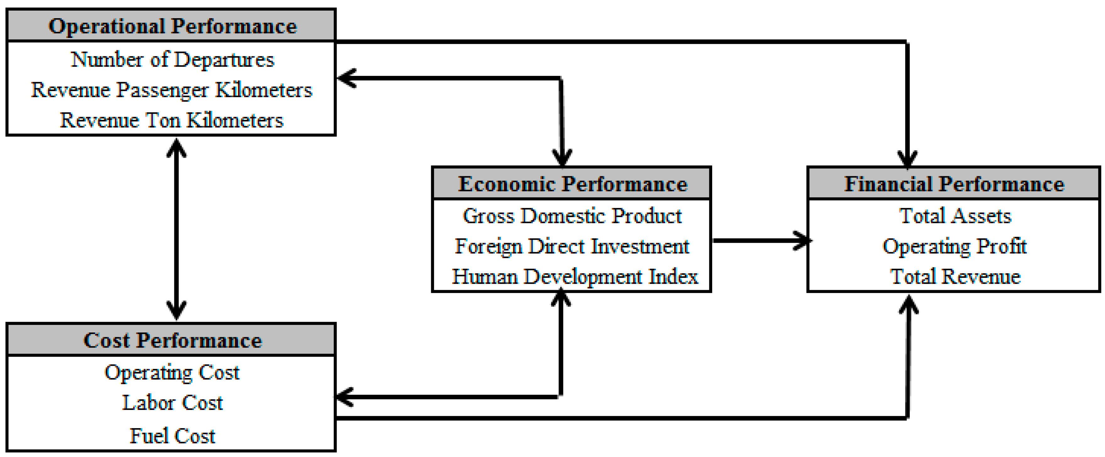
• H₁: Economic performance has a significant impact on financial performance.

Operational performance measures have been broadly applied by a good number of corporations since the early 1990s to measure current performance, identify requirements needed to enhance performance, and make the achievement of far-fetched strategic goals possible [53]. Recently, operational performance measures have been able to gain a global prevalence as myriad organizations and companies around the world have shifted their attention and reliance from the traditional method based mainly on financial performance measures to a range of non-traditional value indices [54]. Revenue passenger kilometer, revenue tone kilometer [55,56], and number of departures [6] are the main operational performance indicators in the airline industry. In our study, we define operational performance with a combination of these three indicators. Logically and empirically operational performance has an impact on financial performance and the relationship between economic performance and operational performance is confirmed by previous studies [57]. Therefore, we considered these relations in the research model and tested the following hypotheses:

• H₂: Operational performance has a significant impact on financial performance.
• H₃: There is a significant relationship between economic performance and operational performance.

Cost function is another type of airline sustainability study. In this type of study, researchers consider cost indicators of two types. The first type cost indicator is a function of operational performance:

Cost indicator = f (operational indicators)

Zuidberg [7] and Hansen, Gillen [11] have done their modeling based on the above function. The second type is a financial indicator and it is a function of cost and operational indicators;

Financial indicator = f (cost indicators, operational indicators)

Johnston and Ozment [9] and Oum and Zhang [10] have done their modeling based on the above function. However, the combination of two types of modeling, especially with the leveraging of country economic performance, is rare. Therefore, this study considers cost performance as the fourth latent variable with a combination of operating cost, labor cost, and fuel cost indicators based on the Zuidberg [7] study. Considering this latent variable lead to the development in our study of the following hypotheses:

• H₄: Cost performance has significant impact on financial performance.
• H₅: There is a significant relationship between cost performance and operational performance.
• H₆: There is a significant relationship between economic performance and cost performance.

Figure 2 shows the hypothesized research model with the latent variables, while their indicators serve to show the impact of economic performance with both cost performance and operational performance on financial performance. The figure illustrates that the first three constructs are interrelated. As a result, the present research model includes four constructs and twelve observed variables.

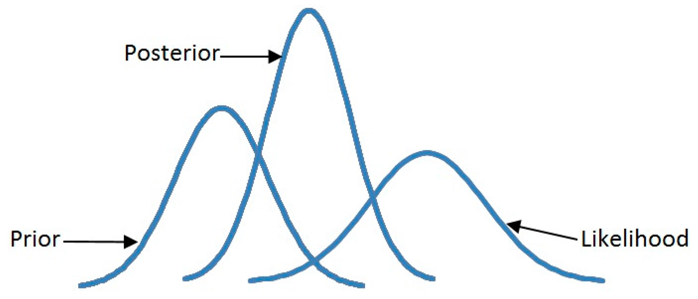
3. Classical-SEM & Bayesian-SEM Theories

To perform statistical analysis, classical as well as Bayesian paradigms are initially used. According to traditional principles, supposing the parameter of interest $\mathbf{\Theta }$ is constant (non-stochastic), inferential subjects about $\mathbf{\Theta }$ are handled based on likelihood/log-likelihood. If the likelihood is denoted by $L(\mathbf{\Theta })$, it is assumed that the information about $\mathbf{\Theta }$ can be obtained only through sample $x\in \mathrm{X},$ and the likelihood is a function of $\mathbf{\Theta }$ conditional on the observed value of $X$. However, by adopting the Bayesian paradigm, it can be assumed that $\Theta$ is stochastic and it can be incorporated in the model as a random variable. In this regard, $\mathbf{\Theta }$ has a probability measure $\pi (\mathbf{\Theta })$, or a prior distribution that gives more information about the parameter than likelihood. The information may be from different sources such as physical reasoning or expert views. Then the information in $\pi (\mathbf{\Theta })$ about $\mathbf{\Theta }$ can be updated using the likelihood information, yielding the posterior distribution denoted by $\pi (\mathbf{\Theta }|\mathit{X}=x)$. From a Bayesian point of view, an inference about $\mathbf{\Theta }$ can only be made through posterior distribution.

Note that the likelihood can be considered as the distribution of the data given the parameter value. Based on Figure 3, the major portion of the prior distribution has a lower parameter value than that at the peak of the likelihood. The posterior is obtained as a compromise between the prior and the likelihood.

There are three main types of prior probability distributions (informative, uninformative, and weakly informative) that vary in their degree of (un)certainty about the parameter of interest in the research model [59]. Applying informative priors means employing data from theories, literature, expert opinion, or previous experiments. Informative priors can have a significant influence on the final parameter estimates. Uninformative priors are considered by the researchers when there is no prior knowledge about the parameter of interest [60]. A compromise between the informative and uninformative priors is called a weakly informative prior [61,62,63]. Weakly informative priors can be recommended when the researchers want to apply a weakerer prior than what your actual knowledge would allow [62]. Weakly informative priors include some information about the parameter estimate but do not typically impact the final parameter estimate to a large extent. In our research model, we do not have any prior knowledge about the parameter of interested, therefore, the uninformative priors are specified.

In what follows, each analysis is specifically addressed. From a conventional viewpoint, the classical SEM is initially specified, and the measurement and structural relations are defined. Suppose that the measurement equation is

$${\mathit{x}}_{\mathit{i}}=\mathbf{\Lambda }{\mathit{\omega }}_{\mathit{i}}+{\mathit{\epsilon }}_{\mathit{i}}; i=1,2,\dots ,n$$

where ${\mathit{x}}_{\mathit{i}}$ is a $p\times 1$ vector of indicators describing the $q\times 1$ random vector of latent variable ${\mathit{\omega }}_{\mathit{i}}$; $\mathbf{\Lambda }$ is a $p\times q$ matrix of the loading coefficients obtained from the regressions of ${\mathit{x}}_{\mathit{i}}$ on ${\mathit{\omega }}_{\mathit{i}}$; and ${\mathit{\epsilon }}_{\mathit{i}}$ is $p\times 1$ represents random vectors of the measurement errors that are summed to be the distribution according to $N\left(0,{\mathit{\psi }}_{\mathit{\epsilon }}\right)$ in the current setup. It is further assumed that vectors ${\mathit{\omega }}_{\mathit{i}}$, $i=1,\dots ,n$ are independent, uncorrelated with ${\mathit{\epsilon }}_{\mathit{i}}$, and specifically distributed according to $N\left(0,\mathbf{\Phi }\right)$. To accommodate the relation between endogenous and exogenous variables, ${\mathit{\omega }}_{\mathit{i}}$ is partitioned as $\left({\mathit{\eta }}_{\mathit{i}},{\mathit{\xi }}_{\mathit{i}}\right)$, where ${\mathit{\eta }}_{\mathit{i}}$ and ${\mathit{\xi }}_{\mathit{i}}$ are the $m\times 1$ and $n\times 1$ vectors of the latent variables, respectively.

At this stage, the following structural equation is considered:

$${\mathit{\eta }}_{\mathit{i}}=\mathit{B}{\mathit{\eta }}_{\mathit{i}}+\mathit{\Gamma }{\mathit{\xi }}_{\mathit{i}}+{\mathit{\delta }}_{\mathit{i}}; i=1,2,\dots ,n$$

where $\mathit{B}$ is the $m\times m$ matrix of the structural parameters governing the relationship among endogenous latent variables, which is assumed to have zeros in the diagonal; $\mathit{\Gamma }$ is the $m\times n$ regression parameter matrix for relating the endogenous with exogenous latent variables; and ${\mathit{\delta }}_{\mathit{i}}$ is the $m\times 1$ vector of disturbances, which is assumed to be distributed according to $N\left(0,{\mathit{\psi }}_{\mathit{\delta }}\right)$ where ${\mathit{\psi }}_{\mathit{\delta }}$ is a diagonal covariance matrix. It is further assumed that ${\mathit{\delta }}_{\mathit{i}}$ is uncorrelated with ${\mathit{\xi }}_{\mathit{i}}$. Since only one endogenous latent variable is involved in this study, in other words, $\mathit{B}{\mathit{\eta }}_{\mathit{i}}=0$, The above formula can be rewritten as ${\mathit{\eta }}_{\mathit{i}}=\mathit{\Gamma }{\mathit{\xi }}_{\mathit{i}}+{\mathit{\delta }}_{\mathit{i}}$ for simplicity.

In this study, for estimating research model parameters based on the SEM technique, the robust weighted least-squares (RWLS) estimation method is incorporated. RWLS provides parameter estimates and standard errors and computes ${\chi }^2$ and the fit indices that are found using the diagonal components of the weight matrix and that are derived based on the threshold asymptotic variances and latent correlation estimates [64]. After the estimation process, model evaluation is required. In this respect, the model’s goodness of fit can be checked through the related Chi-square statistic [CMIN], Normed fit index [NFI], Comparative fit index [CFI], Tucker Lewis index [TLI], Incremental fit index [IFI], Relative fit index [RFI], and goodness of fit index [GFI] [65]. The judgment based on these measures is discussed in detail in the empirical study section.

For perfect SEM analysis and to improve the fit, the model can be modified using ${\chi }^2$ difference, Lagrange multiplier, and Wald tests. Many programs provide modification indices that specify the fit improvement as a result of adding an extra path to the model [65].

From a Bayesian viewpoint, the prior distribution must first be specified. Beforehand, similar to Yanuar, Ibrahim [66], a threshold specification has to be identified in order to treat the ordered categorical data as manifestations of hidden continuous normal distribution. As a brief explanation about threshold specification, if adopting the parameterization by Lee [38], suppose $\mathit{X}=\left({\mathit{x}}_{\mathbf{1}},{\mathit{x}}_{\mathbf{2}},\dots ,{\mathit{x}}_{\mathit{n}}\right)$ and $\mathit{Y}=\left({\mathit{y}}_{\mathbf{1}},{\mathit{y}}_{\mathbf{2}},\dots ,{\mathit{y}}_{\mathit{n}}\right)$ are both latent continuous variables. The relationship between $\mathit{X}$ and $\mathit{Y}$ is explained using the threshold specification. The procedure for $x_1$ is described as an instant. More precisely, let

$${\mathit{x}}_{\mathbf{1}}=c if {\tau }_c-1<{\mathit{y}}_{\mathbf{1}}<{\tau }_c,$$

where $c$ is the number of categories for ${\mathit{x}}_{\mathbf{1}}$, and ${\tau }_c-1$ and ${\tau }_c$ denote the threshold levels associated with ${\mathit{y}}_{\mathbf{1}}$. For example, in this study $c=3$ is considered, where ${\tau }_0=-\infty$ and ${\tau }_3=\infty$. Meanwhile, the values of ${\tau }_1$ and ${\tau }_2$ are determined based on the proportion of cases in each category of $x_1$ using

$${\tau }_k={\mathbf{\Phi }}^{-1}({\sum }_{r=1}^2\frac{N_r}{N}), k=1,2,$$

where ${\mathbf{\Phi }}^{-1}(\cdot )$ is the inverse of the standardized normal distribution, $N_r$ is the number of cases in the $r$th category and $N$ is the total number of cases. It is specifically assumed that $\mathit{Y}$ is distributed according to a multivariate normal.

Under the Bayesian-SEM, $\mathit{X}=\left({\mathit{x}}_{\mathbf{1}},{\mathit{x}}_{\mathbf{2}},\dots ,{\mathit{x}}_{\mathit{n}}\right)$ and $\mathit{Y}=\left({\mathit{y}}_{\mathbf{1}},{\mathit{y}}_{\mathbf{2}},\dots ,{\mathit{y}}_{\mathit{n}}\right)$ are continuous data matrices and latent continuous variables, respectively, and $\mathbf{\Omega }=\left({\mathit{\omega }}_{\mathbf{1}},{\mathit{\omega }}_{\mathbf{2}},\dots ,{\mathit{\omega }}_{\mathit{n}}\right)$ is the matrix of latent variables. The observed data $\mathit{X}$ are augmented with the latent data $\left(\mathit{Y}, \mathbf{\Omega }\right)$ in the posterior analysis. The parameter space is denoted by $\mathbf{\Theta }=\left(\mathit{\tau },\mathit{\theta },\mathbf{\Omega }\right)$, where $\mathit{\theta }=\left(\mathbf{\Phi },\mathbf{\Lambda },{\mathbf{\Lambda }}_{\mathit{\omega }},{\mathbf{\Psi }}_{\mathit{\delta }},{\mathbf{\Psi }}_{\mathit{\epsilon }}\right)$ is the structural parameter. In line with Lee [38], the prior model is given by

$$\pi (\mathbf{\Theta })=\pi \left(\mathit{\tau }\right)\pi \left(\mathit{\theta }\right)\pi (\mathbf{\Omega }|\mathsf{\tau },\mathsf{\theta })$$

where due to the ordinal nature of thresholds, a diffuse prior can be adopted. Specifically, for some constant $c$,

$$\pi \left(\mathit{\tau }\right)=c$$

Further, to accommodate a subjective viewpoint, a natural conjugate prior can be adopted for $\mathit{\theta }$ with the conditional representation $\pi \left(\mathit{\theta }\right)=\pi \left(\mathbf{\Lambda }|{\mathbf{\Psi }}_{\mathit{\epsilon }}\right)\pi \left({\mathbf{\Psi }}_{\mathit{\epsilon }}\right)$. More specifically, let

$$\left({\Lambda }_k|{\psi }_{\epsilon k}^{-1}\right)\sim N\left({\Lambda }_{0k},{\psi }_{\epsilon k} {\mathit{H}}_{\mathbf{0}\mathit{y}\mathit{k}}\right), {\psi }_{\epsilon k}^{-1}\sim \Gamma \left({\alpha }_{0\epsilon k},{\beta }_{0\epsilon k}\right)$$

where ${\psi }_{\epsilon k}$ is the kth diagonal element of ${\psi }_{\epsilon }$, ${\Lambda }_k$ is the $k$th row of $\mathbf{\Lambda }$, and $\Gamma$ denotes the gamma distribution. Finally, an inverse-Wishart distribution is adopted for $\Phi$ as follows:

$${\mathbf{\Phi }}^{-1}\sim W_q\left(R_0,{\rho }_0\right)$$

It is further supposed that all hyperparameters are known. Posterior distribution can be found by normalizing the product $L\left(\mathbf{\Theta }|\mathit{X}=x\right)\pi (\mathbf{\Theta })$.

Owing to computational difficulties in identifying the posterior distribution $\mathbf{\Theta }|\mathit{X}=x$, the Markov Chain Monte Carlo (MCMC) technique is applied to generate a sequence of random observations from $\mathbf{\Theta }|\mathit{X}=x$. Then Bayesian analysis can be performed using WinBUGS, a freely available software.

The next procedure in Bayesian-SEM is convergence testing of the research model parameters. According to Yanuar, Ibrahim [67], model diagnostics are performed by graphically designing time series diagrams to evaluate the accuracy of the research parameters with different starting values and to illustrate the diagnosis based on tracing of the diagrams [39,68].

To assess the plausibility of the proposed model, which includes measurement and structural equations, the residual estimates are plotted versus the latent variable estimates to provide information on the model fit. The residual estimates for measurement equation (${\widehat{\mathit{\epsilon }}}_{\mathit{i}}$) can be obtained from

$${\widehat{\mathit{\epsilon }}}_{\mathit{i}}={\mathit{y}}_{\mathit{i}}-\widehat{\mathbf{\Lambda }}{\widehat{\mathit{\xi }}}_{\mathit{i}}, i=1,2,\dots ,n,$$

where $\widehat{\mathbf{\Lambda }}$ and ${\widehat{\mathit{\xi }}}_{\mathit{i}}$ are Bayesian estimates obtained via the MCMC methods. The estimates of residuals in structural equation (${\widehat{\mathit{\delta }}}_{\mathit{i}}$) can be obtained from the following estimated model:

$${\widehat{\mathit{\delta }}}_{\mathit{i}}=\left(\mathit{I}-\widehat{\mathit{B}}\right){\widehat{\mathit{\eta }}}_i-\widehat{\mathbf{\Gamma }}{\widehat{\mathit{\xi }}}_i, i=1,2,\dots ,n,$$

where $\widehat{\mathit{B}}$, ${\widehat{\mathit{\eta }}}_{\mathit{i}}$, $\widehat{\mathbf{\Gamma }}$ and ${\widehat{\mathit{\xi }}}_{\mathit{i}}$ are Bayesian estimates obtained from the corresponding simulated observations through MCMC.

According to Figure 2, the model hypothesized in this study consists of 12 indicator variables with three exogenous latent variables and one endogenous latent variable. The following measurement model is then formulated:

$${\mathit{y}}_{\mathit{i}}=\mathbf{\Lambda }{\mathit{\omega }}_{\mathit{i}}+{\mathit{\epsilon }}_{\mathit{i}}, i=1,2,\dots ,n,$$

where ${\mathit{\omega }}_{\mathit{i}}={\left({\mathit{\eta }}_{\mathit{i}},{\mathit{\xi }}_{\mathit{i}\mathbf{1}},{\mathit{\xi }}_{\mathit{i}\mathbf{2}},{\mathit{\xi }}_{\mathit{i}\mathbf{3}}\right)}^T$. The structural part of the current SEM model has the form

$${\mathit{\eta }}_{\mathit{i}}={\gamma }_1 {\mathit{\xi }}_{\mathit{i}\mathbf{1}}+{\gamma }_2{\mathit{\xi }}_{\mathit{i}\mathbf{2}}+{\gamma }_3{\mathit{\xi }}_{\mathit{i}\mathbf{3}}+{\mathit{\delta }}_{\mathit{i}},$$

where ${\left({\mathit{\xi }}_{\mathit{i}\mathbf{1}},{\mathit{\xi }}_{\mathit{i}\mathbf{2}},{\mathit{\xi }}_{\mathit{i}\mathbf{3}}\right)}^T$ is distributed as $N\left(0,\mathbf{\Phi }\right)$ and independent with ${\mathit{\delta }}_{\mathit{i}}$ which is distributed as $N\left(0,{\mathit{\psi }}_{\mathit{\delta }}\right)$.

In the data analysis, AMOS 18 is used to estimate the parameters for Classical-SEM, while the Bayesian model is fitted to the data using winBUGS version 1.4.

4. Materials and Methods

Based on an Air Transport World (ATW) report from 2013 [69], 106 airlines were listed in the Asia-Pacific region.

Nevertheless, it is notable to mention that airline companies are classified as a service-providing sector whose main task includes service provision to their customers. These types of airlines are categorized into three groups in terms of service type: airline companies specializing in transfer of passengers, airline companies specializing in cargo transfer, and airline companies specializing in both passenger and cargo transfer. This paper, however, only focuses on the airline firms specializing in passenger transfer although they also concurrently provide services for cargo transfer. The cargo transferring aspects of the case have been excluded from the present research domain (four companies). Moreover, nineteen low-cost airline carriers were eliminated from the present research domain (nineteen companies). Therefore, 23 companies that are trunk and low-cost carriers were excluded from the present research domain. In this study, 30 (36%) airline companies were selected over a 10-year period (2006 to 2015). The data were reported on an annual basis and gathered from an overall company level rather than city pairs. Therefore, 300 records were considered, seven of them were deleted due to missing information.

Mahalanobis distance is an extremely general measure that is utilized for measurement of multivariate outliers [70]. Based on Mahalanobis distance testing, ten observations (observation number; 9, 32, 39, 86, 103, 122, 209, 252, 265, and 271) were eliminated from the list because they were considered as outliers, which could affect the model fit, R², and the size and direction of parameter estimates (see

Table 1. The analysis of Mahalanobis distance.

Observation Number	Mahalanobis D-Squared	p1	p2
9	86.25	0.0044	0.0086
32	69.12	0.0068	0.0092
39	63.22	0.0099	0.0112
86	61.59	0.0109	0.0188
103	45.12	0.0182	0.0219
122	36.18	0.0367	0.0286
209	22.19	0.0394	0.0411
252	20.91	0.0421	0.0569
265	13.25	0.0467	0.0758
271	10.37	0.0483	0.1024

Note: If p1 or p2 is less than 0.05 then the observation is an outlier.

). Therefore, (300 − 7 − 10 = 283) observations were considered in the final data of the study.

5. Results

Figure 4 represents the results of model fitting based on the SEM approach. The values of GFI, IFI, TLI, and NFI are within the acceptable range. Therefore, the current model is fitted for our data at the 5% significance level.

Controlling for outliers and maintaining normal distribution support in adjusting the heterogeneity of the research data. The employment of the maximum likelihood estimator in this study uses the Classical-SEM procedure. The main essential assumption for the employment of the maximum likelihood is that the data are required to follow normal distribution and the scale of observed variables must be continuous. The normality testing that should be used in Classical-SEM is based on the value of skewness and kurtosis. If the absolute kurtosis value is less than 7 and the value of skewness is between −2 and +2, the endogenous variables normality is acceptable. Based on

Table 2. Normality test.

Variable	Skew	C.R.	Kurtosis	C.R.
Number of Departures	3.063	9.549	8.640	12.775
Revenue Passenger Kilometers	2.361	7.130	7.396	10.719
Revenue Ton Kilometers	2.938	7.936	9.311	14.033
Gross Domestic Product	0.243	2.106	−0.299	−1.299
Foreign Direct Investment	−0.036	−0.313	−0.615	−2.669
Human Development Index	−0.010	−0.083	−0.677	−2.939
Operating Cost	−0.044	−0.382	−0.815	−3.538
Labor Cost	0.181	1.569	−1.217	−5.280
Fuel Cost	0.687	5.959	0.471	2.046
Total Assets	0.259	2.252	−0.404	−1.754
Operating Profit	−0.080	−0.695	−0.479	−2.080
Total Revenue	−0.099	−0.855	−0.459	−1.992

Note: Critical Ratio (C.R.).

, revenue passenger kilometer, revenue ton kilometers, and number of departures are not normally distributed. Moreover, based on the output of the multivariate normality test, the kurtosis value is 18.69, and this value is not less than 10. Therefore, the multivariate normality hypothesis is rejected [71].

Table 3. Estimated parameters of SEM using Maximum Likelihood and Bayesian predictors.

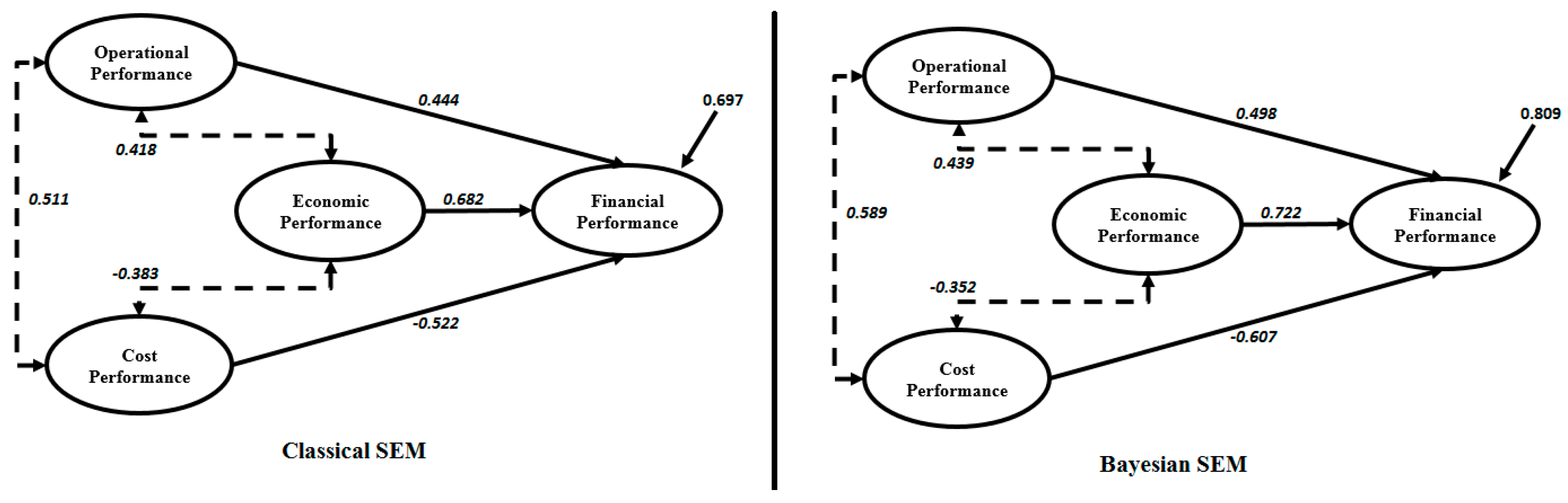
Relation	Estimated Coefficients
	Classical SEM	Bayesian SEM
Economic Performance → Financial Performance	0.682 *	0.722 *
Operational Performance → Financial Performance	0.444 *	0.498 *
Cost Performance → Financial Performance	−0.522 *	−0.607 *
Economic Performance ↔ Operational Performance	0.418 *	0.439 *
Economic Performance ↔ Cost Performance	−0.383 *	−0.352 *
Operational Performance ↔ Cost Performance	0.511 *	0.589 *

* Presents significant relation with 95% confidence.

and Figure 5 present the output of research hypotheses regarding the relationship among the variables. The convergence statistics tests for each parameter of interest show that the R² values were approximately 1. In both models, the impact of economic performance $({\beta }_{Classical}=0.682; {\beta }_{Bayesian}=0.722;p-value<0.05)$ and operational performance $({\beta }_{Classical}=0.444; {\beta }_{Bayesian}=0.498;p-value<0.05)$ on financial performance are significant and positive. However, the impact of cost performance $({\beta }_{Classical}=-0.522; {\beta }_{Bayesian}=-0.607;p-value<0.05)$ on financial performance is significant and negative. Moreover, the relationships between operational performance with both economic performance $({\beta }_{Classical}=0.418; {\beta }_{Bayesian}=0.439;p-value<0.05)$ and cost performance $({\beta }_{Classical}=0.511; {\beta }_{Bayesian}=0.589;p-value<0.05)$ is significant and positive, and the relationship between economic performance and cost performance is significant and negative $({\beta }_{Classical}=-0.383; {\beta }_{Bayesian}=-0.352;p-value<0.05)$.

Based on Figure 5, the estimated structural equations were obtained that addressed the relationship between the performance index with economic performance, operational performance, and cost performance for the Classical-SEM and Bayesian-SEM, respectively given by

$$\widehat{\eta }\left(Classical-SEM\right)=0.682{\zeta }_1-0.522{\zeta }_2+0.444{\zeta }_3$$

and

$$\widehat{\eta }\left(Bayesian-SEM\right)=0.722{\zeta }_1-0.607{\zeta }_2+0.498{\zeta }_3$$

Based on the estimated structural equations, it is concluded that economic performance (ξ1) has the most influence on financial performance (η) compared with the other latent variables. In brief, cost performance and operational performance are highly linked to financial performance, showing that better leadership strategies are more able to produce a high quality performance status.

Table 4. Factor loading, Standard Error [S.E] and confidence interval (CI) of indicators in the measurement model.

	Factor Loading, [S.E] and (CI)
Measurement Variable	Classical-SEM	Bayesian-SEM
Economic Performance
Foreign Direct Investment	1	1
Gross Domestic Products	0.666 * [0.078] (0.532, 0.789)	0.509 * [0.071] (0.421, 0.631)
Human Development Index	0.845 * [0.352] (0.721, 0.936)	0.812 * [0.342] (0.744, 0.859)
Operational Performance
Number of Departures	1	1
Revenue Passenger Kilometers	0.688 * [0.138] (0.598, 0.759)	0.695 * [0.133] (0.613, 0.742)
Revenue Ton Kilometers	0.712 * [0.096] (0.589, 0.796)	0.716 * [0.091] (0.607, 0.788)
Cost Performance
Operating Cost	1	1
Labor Cost	0.798 * [0.076] (0.683, 0.843)	0.799 * [0.074] (0.691, 0.837)
Fuel Cost	0.671 * [0.109] (0.598, 0.711)	0.684 * [0.102] (0.611, 0.706)
Financial Performance
Total Assets	1	1
Operating Profit	0.823 * [0.031] (0.729, 0.868)	0.811 * [0.029] (0.741, 0.855)
Total Revenue	0.745 * [0.056] (0.656, 0.807)	0.751 * [0.044] (0.631, 0.802)

* Significant in the level of 5%; CI: Confidence Interval.

presents the values of factor loading regulated coefficients and related standard errors for every indicator variable in the measurement equations acquired through both methods. It is clear from Table 4 that both models produced nearly the same factor loading estimates. It should also be mentioned that the indicator variables speculated as predictors are remarkably associated with their specific latent factors. It is highly significant that the parameter estimate standard errors under Bayesian-SEM are lower than under Classical-SEM. Moreover, Table 4 indicates that the 95% confidence intervals related to the parameters achieved with Bayesian-SEM are mainly shorter than that of the Classical-SEM-based parameters, which is not unordinary in light of the data provided by the prior distribution.

This part of the study presents the comparison analysis between the Classical-SEM and Bayesian-SEM techniques in predicting the airline financial performance index. Four mathematical indices were applied to compare the Bayesian-SEM and Classical-SEM, which are representative of the strength and correctness of the prediction analysis. Root mean square error (RMSE), mean absolute percentage error (MAPE), coefficient of determination (R²), and mean absolute error (MSE) are the most familiar indices for a comparison study among different prediction techniques.

Table 5. Comparative outputs of Classical-SEM and Bayesian-SEM.

Index	Formula	Bayesian-SEM	Classical-SEM
MAPE	$\frac{1}{n}{\sum }_{i = 1}^n\left|\frac{y_i^{\prime }-y_i}{y_i}\right|$	0.158	0.201
RMSE	$\sqrt[2]{\frac{{\sum }_{i = 1}^n{\left(y_i^{\prime }-y_i\right)}^2}{n}}$	0.185	0.199
MSE	$\frac{{\sum }_{i = 1}^n\left|y_i^{\prime }-y_i\right|}{n}$	0.109	0.133
R2	$\frac{{[{\sum }_{i = 1}^n\left(y_i^{\prime }-{\overline{y}}_i^{\prime }\right).\left(y_i-{\overline{y}}_i\right)]}^2}{{\sum }_{i = 1}^n\left(y_i^{\prime }-{\overline{y}}_i^{\prime }\right).{\sum }_{i = 1}^n\left(y_i-{\overline{y}}_i\right)}$	0.809	0.697

presents the formula indices and output in traditional and Bayesian approaches.

In the formulas which are mentioned in Table 5, $y_i$ is the ith real value of the dependent variable ($y$) and $y_i^{\prime }$ is the ith predicted value. The R² value for the Bayesian-SEM model is bigger than the Classical-SEM, and the RMSE, MSE and MAPE values of the Bayesian-SEM are smaller than the Classical-SEM. Therefore, the performance indices with the Bayesian-SEM are better in predicting financial performance than the Classical-SEM. The main reason Bayesian-SEM performs better is the defined traditional framework, which permits simultaneous self-adjustment of parameters and effective learning of the association between inputs and outputs in causal and complex models.

6. Discussion

The main purpose of the present study was to demonstrate the values of the Classical-SEM and Bayesian-SEM techniques in a new airline sustainability framework with the financial performance index for the Asia-Pacific airline industry. The new framework was developed based on previous studies in airline sustainability modeling. The designed model includes four latent variables and twelve familiar indicators. Even though much research has been conducted to determine the airlines’ performance index and airline cost function, not many works have addressed modeling this index using SEM, particularly with interconnection among economic performance, operational performance and cost performance. This study was determined that economic performance should be considered as an independent latent variable in relationship to both operational performance and cost performance. This latent variable includes foreign direct investment, gross domestic products, and human development index. The combination of these three indicators into an economic performance index can directly and indirectly (through cost performance and operational performance) affect the airline financial performance index. Based on the data analysis output, it was found that economic performance has a significant effect on the financial performance index. These findings are similar to studies by Jenatabadi and Ismail [14] and Ismail and Jenatabadi [8] on airline performance modeling with Classical-SEM methodology and studies by Wang and Heinonen [72] who considered effective economic indicators as including gross domestic products and foreign direct investment in their research models. The significant interconnections of three main predictors are approved. It means the relationship between economic performance and operational performance, economic performance and cost performance, and operational performance and cost performance are significant. Moreover, the impact of every one of those three predictors on financial performance are significant. Therefore, the designed framework includes the impact of three predictors and the interconnection among them on financial performance is fitted to the current data.

The data were only collected in the Asia Pacific region, therefore, the findings cannot be generalized to all airlines in the world. However, the model proposed in this study has a potential capability and ability to be applied to airline companies. In this model, in order to enhance its efficiency, all redundant measures were eliminated or modified to be as close to the requirements of the airline industry as possible. The results of data analysis verified that the model consisting of four constructs was effective in understanding their role in predicting and estimating financial performance. The final model, which has a potential to be used in airline companies, is extremely close to the needs and the requirements of the industry as all redundant measures were eliminated and the most used and proper ones were added as measures and indicators.

This information should be helpful for managers and decision-makers to distribute capital resources logically upon implementing plans to improve the overall company performance. This information can be condensed in a single measure called a performance index, which is essential for detecting the indicators that could have an impact on it.

The other part of the main objective of this study was to illustrate Bayesian-SEM for analyzing the airline performance index. Along the lines of maximum likelihood and considering the Bayesian concept, the research parameters were defined as random with a prior distribution and prior density function [38]. After gathering data, the first phase in applying the Bayes theorem entailed combining these with prior distributions. The next phase was to calculate the posterior distribution, which reveals prior knowledge and empirical research data. By performing MCMC simulation, it was possible to summarize the joint posterior distribution with regard to lower dimensional summary statistics like posterior mean and standard deviation. Therefore, Bayesian application in SEM studies is more suitable for our research data.

A computational algorithm in Classical-SEM was determined based on a normality assumption and the sample covariance matrix of the research data. However, in many studies identified, multivariate normality was not the researchers’ concern or the data did not have a normal structure. Therefore, researchers including Bashir and Schilizzi [73], Ansari, Jedidi [68], and Scheines, Hoijtink [39] considered that the Bayesian approach in SEM has the capability to overcome the non-normality concern.

Unit heteroscedasticity leads to damage of the homoscedastic error assumptions [74]. Heteroscedasticity is treated quite differently in the Bayesian context relative to maximum likelihood. Since our estimate of uncertainty is considered from the posterior distribution, we only have to be concerned about fittingly modeling the process to measure that distribution correctly. In a maximum based estimator, researchers would reweight the standard errors based on group size, however, within a Bayesian framework, the inferences on each parameter fully take into consideration the uncertainty of every other parameter interested. Therefore, as long as we have heterogeneity in the contributed research model, one usually ignores the idea of heteroscedasticity.

7. Conclusions

Based on the structure objective of the study we have two main conclusions. The first conclusion is about the main advantages of the current framework with previous studies in airline sustainability modeling. These advantages are:

• This study developed Jenatabadi and Ismail [14] and Ismail and Jenatabadi [8] in estimating airline performance with application of Classical-SEM by interfering cost performance and considering operational performance separate from financial performance in different latent variables.
• This study developed previous studies like Johnston and Ozment [9], Oum and Zhang [10], Zuidberg [7], and Hansen, Gillen [11] in airline sustainability performance in terms of cost function by leveraging country economic performance indicators.

The second conclusion is that based on the value of R² in Table 5, we can interpret from the Bayesian-SEM of 80.9% that variation in financial performance is related to economic performance, cost performance, and operational performance. However, this variation based on Classical-SEM is equal 67.9%. Moreover, based on the values of MPE, RMSE, and MSE, the amount of residuals of Bayesian-SEM are less than that of Classical-SEM. It means the predicted values of Bayesian-SEM are closer to the observed value than that of Classical-SEM. As a result, with higher values of R² and lower values of MPE, RMSE, and MSE, Bayesian-SEM have a better goodness of fit for the observations than that of the Classical-SEM.

This study does have its limitations from a practical standpoint of airline sustainability modeling structure. The main limitation is the exclusion of a few essential indicators such as ticket price, top management team, customer satisfaction, and governmental subsidy. Ticket price has been used in price modelling [75], choice modelling [76,77], and performance estimating [47]. For airline sustainability modelling, this indicator is suitable for the city pair level and not at the industrial level. For this reason, ticket price is also excluded from our research model. Information of top management team and customer satisfaction are also not available in the annual report and, therefore, are excluded from the research model. The governmental subsidy is financial support given to some airline companies by their governments [78]. The subsidy given by the government allows companies to give discounts to the ticket price for certain air travelers and has the potential to increase the load factor [79].

For future studies the following subjects are recommended:

(1)

Application of the framework which is introduced in Figure 2 in other areas and do comparison study between them.

(2)

Comparison study between Classical-SEM (as representative of parametric modeling) and Bayesian-SEM (as a representative semi-parametric modeling) was done, but comparison between these two methods with artificial neural networks (as a representative of non-parametric modeling) could be an interesting topic for future research.

(3)

Doing comparison analysis with the leveraging governmental subsidy as the main moderator in the research framework of Figure 2.

References

- Schosser, M.; Wittmer, A. Cost and revenue synergies in airline mergers—Examining geographical differences. J. Air Transp. Manag. 2015, 47, 142–153. [Google Scholar] [CrossRef]
- Barbot, C.; Costa, Á.; Sochirca, E. Airlines performance in the new market context: A comparative productivity and efficiency analysis. J. Air Transp. Manag. 2008, 14, 270–274. [Google Scholar] [CrossRef]
- Gudmundsson, S.V. Airline failure and distress prediction: A comparison of quantitative and qualitative models. Transp. Res. Part E Logist. Transp. Rev. 1999, 35, 155–182. [Google Scholar] [CrossRef]
- Cao, Q.; Lv, J.; Zhang, J. Productivity efficiency analysis of the airlines in China after deregulation. J. Air Transp. Manag. 2015, 42, 135–140. [Google Scholar] [CrossRef]
- Hsu, C.I.; Wen, Y.H. Application of grey theory and multiobjective programming towards airline network design. Eur. J. Oper. Res. 2000, 127, 44–68. [Google Scholar] [CrossRef]
- Lee, B.L.; Worthington, A.C. Technical efficiency of mainstream airlines and low-cost carriers: New evidence using bootstrap data envelopment analysis truncated regression. J. Air Transp. Manag. 2014, 38, 15–20. [Google Scholar] [CrossRef]
- Zuidberg, J. Identifying airline cost economies: An econometric analysis of the factors affecting aircraft operating costs. J. Air Transp. Manag. 2014, 40, 86–95. [Google Scholar] [CrossRef]
- Ismail, N.A.; Jenatabadi, H.S. The influence of firm age on the relationships of airline performance, economic situation and internal operation. Transp. Res. Part. A Policy Pract. 2014, 67, 212–224. [Google Scholar] [CrossRef]
- Johnston, A.; Ozment, J. Economies of scale in the US airline industry. Transp. Res. Part E Logist. Transp. Rev. 2013, 51, 95–108. [Google Scholar] [CrossRef]
- Oum, T.H.; Zhang, Y. Utilisation of quasi-fixed inputs and estimation of cost functions: An application to airline costs. J. Transp. Econ. Policy 1991, 121–134. [Google Scholar]
- Hansen, M.M.; Gillen, D.; Djafarian-Tehrani, R. Aviation infrastructure performance and airline cost: A statistical cost estimation approach. Transp. Res. Part E Logist. Transp. Rev. 2001, 37, 1–23. [Google Scholar] [CrossRef]
- Craig, R.; Amernic, J. A privatization success story: Accounting and narrative expression over time. Account. Audit. Account. J. 2008, 21, 1085–1115. [Google Scholar] [CrossRef]
- Halpern, N.; Graham, A. Airport route development: A survey of current practice. Tour. Manag. 2015, 46, 213–221. [Google Scholar] [CrossRef]
- Jenatabadi, H.S.; Ismail, N.A. Application of structural equation modelling for estimating airline performance. J. Air Transp. Manag. 2014, 40, 25–33. [Google Scholar] [CrossRef]
- Bubalo, B.; Gaggero, A.A. Low-cost carrier competition and airline service quality in Europe. Transp. Policy 2015, 43, 23–31. [Google Scholar] [CrossRef]
- Chang, D.S.; Chen, S.H.; Hsu, C.W.; Hu, A.H. Identifying strategic factors of the implantation CSR in the airline industry: The case of Asia-Pacific airlines. Sustainability 2015, 7, 7762–7783. [Google Scholar] [CrossRef]
- Graham, A. Understanding the low cost carrier and airport relationship: A critical analysis of the salient issues. Tour. Manag. 2013, 36, 66–76. [Google Scholar] [CrossRef]
- Navarro, J.L.A.; Martínez, M.E.A.; Trinquecoste, J.F. The effect of the economic crisis on the behaviour of airline ticket prices. A case-study analysis of the New York–Madrid route. J. Air Transp. Manag. 2015, 47, 48–53. [Google Scholar] [CrossRef]
- Kuljanin, J.; Kalić, M. Exploring characteristics of passengers using traditional and low-cost airlines: A case study of Belgrade Airport. J. Air Transp. Manag. 2015, 46, 12–18. [Google Scholar] [CrossRef]
- Hu, Y.; Xiao, J.; Deng, Y.; Xiao, Y.; Wang, S. Domestic air passenger traffic and economic growth in China: Evidence from heterogeneous panel models. J. Air Transp. Manag. 2015, 42, 95–100. [Google Scholar] [CrossRef]
- Zhang, Y. International arrivals to Australia: Determinants and the role of air transport policy. J. Air Transp. Manag. 2015, 44, 21–24. [Google Scholar] [CrossRef]
- Sun, J.Y. Clustered airline flight scheduling: Evidence from airline deregulation in Korea. J. Air Transp. Manag. 2015, 42, 85–94. [Google Scholar] [CrossRef]
- Chung, L.H. Impact of pandemic control over airport economics: Reconciling public health with airport business through a streamlined approach in pandemic control. J. Air Transp. Manag. 2015, 44, 42–53. [Google Scholar] [CrossRef]
- Di Gravio, G.; Mancini, M.; Patriarca, R.; Costantino, F. Overall safety performance of the air traffic management system: Indicators and analysis. J. Air Transp. Manag. 2015, 44, 65–69. [Google Scholar] [CrossRef]
- Augustyniak, W.; López-Torres, L.; Kalinowski, S. Performance of Polish regional airports after accessing the European Union: Does liberalisation impact on airports’ efficiency. J. Air Transp. Manag. 2015, 43, 11–19. [Google Scholar] [CrossRef]
- Mallikarjun, S. Efficiency of US airlines: A strategic operating model. J. Air Transp. Manag. 2015, 43, 46–56. [Google Scholar] [CrossRef]
- Ülkü, T. A comparative efficiency analysis of Spanish and Turkish airports. J. Air Transp. Manag. 2015, 46, 56–68. [Google Scholar] [CrossRef]
- Zou, B.; Kafle, N.; Chang, Y.T.; Park, K. US airport financial reform and its implications for airport efficiency: An exploratory investigation. J. Air Transp. Manag. 2015, 47, 66–78. [Google Scholar] [CrossRef]
- Barros, C.P.; Wanke, P. An analysis of African airlines efficiency with two-stage TOPSIS and neural networks. J. Air Transp. Manag. 2015, 44, 90–102. [Google Scholar] [CrossRef]
- Xiao, Y.; Liu, J.J.; Hu, Y.; Wang, Y.; Lai, K.K.; Wang, S. A neuro-fuzzy combination model based on singular spectrum analysis for air transport demand forecasting. J. Air Transp. Manag. 2014, 39, 1–11. [Google Scholar] [CrossRef]
- Jenatabadi, H.S. Impact of economic performance on organizational capacity and capability: A case study in airline industry. Int. J. Bus. Manag. 2013, 8, 112–120. [Google Scholar]
- Kim, Y.; Yun, S.; Lee, J. Can companies induce sustainable consumption? The impact of knowledge and social embeddedness on airline sustainability programs in the US. Sustainability 2014, 6, 3338–3356. [Google Scholar] [CrossRef]
- Hsu, C.J.; Yen, J.R.; Chang, Y.C.; Woon, H.K. How do the services of low cost carriers affect passengers’ behavioral intentions to revisit a destination? J. Air Transp. Manag. 2016, 52, 111–116. [Google Scholar] [CrossRef]
- Kim, S.L.; Cho, Y.S. Study on Internal Service Quality, Job Satisfaction and Customer Satisfaction in Airline Industry. J. Korea Soc. Comput. Inf. 2016, 21, 113–121. [Google Scholar] [CrossRef]
- Park, E.; Lee, S.; Kwon, S.J.; Del Pobil, A.P. Determinants of behavioral intention to use South Korean airline services: Effects of service quality and corporate social responsibility. Sustainability 2015, 7, 12106–12121. [Google Scholar] [CrossRef]
- Yao, Q.; Xu, M.; Jiang, W.; Zhang, Y. Do marketing and government R&D subsidy support technological innovation? Int. J. Technol. Policy Manag. 2015, 15, 213–225. [Google Scholar]
- Geman, S.; Geman, D. Stochastic relaxation, Gibbs distributions and the Bayesian restoration of images. J. Appl. Stat. 1993, 20, 25–62. [Google Scholar] [CrossRef]
- Lee, S.Y. Structural Equation Modeling: A Bayesian Approach 2007, 1st ed.; John Wiley & Sons: West Sussex, UK, 2007; pp. 24–25. [Google Scholar]
- Scheines, R.; Hoijtink, H.; Boomsma, A. Bayesian estimation and testing of structural equation models. Psychometrika 1999, 64, 37–52. [Google Scholar] [CrossRef]
- Lee, S.Y.; Song, X.Y. Evaluation of the Bayesian and maximum likelihood approaches in analyzing structural equation models with small sample sizes. Multivar. Behav. Res. 2004, 39, 653–686. [Google Scholar] [CrossRef] [PubMed]
- Dunson, D.B. Bayesian latent variable models for clustered mixed outcomes. J. R. Stat. Soc. Ser. B Stat. Methodol. 2000, 62, 355–366. [Google Scholar] [CrossRef]
- Caves, D.W.; Christensen, L.R.; Tretheway, M.W. Economies of density versus economies of scale: Why trunk and local service airline costs differ. Rand J. Econ. 1984, 15, 471–489. [Google Scholar] [CrossRef]
- Sickles, R.C. A nonlinear multivariate error components analysis of technology and specific factor productivity growth with an application to the US Airlines. J. Econom. 1985, 27, 61–78. [Google Scholar] [CrossRef]
- Sickles, R.C.; Good, D.; Johnson, R.L. Allocative distortions and the regulatory transition of the US airline industry. J. Econom. 1986, 33, 143–163. [Google Scholar] [CrossRef]
- Borenstein, S. The dominant-firm advantage in multiproduct industries: Evidence from the US airlines. Q. J. Econ. 1991, 106, 1237–1266. [Google Scholar] [CrossRef]
- Banker, R.D.; Johnston, H.H. An empirical study of the business value of the US airlines’ computerized reservations systems. J. Organ. Comp. Electron. Commer. 1995, 5, 255–275. [Google Scholar]
- Duliba, K.A.; Kauffman, R.J.; Lucas, H.C. Appropriating value from computerized reservation system ownership in the airline industry. Organ Sci. 2001, 12, 702–728. [Google Scholar] [CrossRef]
- Ramanathan, R. The long-run behaviour of transport performance in India: A cointegration approach. Transp. Res. Part A Policy Pract. 2001, 35, 309–320. [Google Scholar] [CrossRef]
- Rangarajan, S.; Prasad, V.A. The Indian airline industry—Will the flight be smooth? Emerald Emerg. Mark. Case Stud. 2014, 4, 1–18. [Google Scholar] [CrossRef]
- Liu, C.M. Entry behaviour and financial distress: An empirical analysis of the US domestic airline industry. J. Transp. Econ. Policy 2009, 43, 237–256. [Google Scholar]
- Barros, C.P.; Couto, E. Productivity analysis of European airlines, 2000–2011. J. Air Transp. Manag. 2013, 31, 11–13. [Google Scholar] [CrossRef]
- Moon, J.; Lee, W.S.; Dattilo, J. Determinants of the payout decision in the airline industry. J. Air Transp. Manag. 2015, 42, 282–288. [Google Scholar] [CrossRef]
- Liedtka, S.L.; Church, B.K.; Ray, M.R. Performance variability, ambiguity intolerance, and balanced scorecard-based performance assessments. Behav. Res. Account. 2008, 20, 73–88. [Google Scholar] [CrossRef]
- Carastro, M.J. Nonfinancial Performance Indicators for US Airlines: A Statistical Analysis. Ph.D. Thesis, University of Phoenix, Tempe, AZ, USA, 2010. [Google Scholar]
- Ouellette, P.; Petit, P.; Tessier-Parent, L.P.; Vigeant, S. Introducing regulation in the measurement of efficiency, with an application to the Canadian air carriers industry. Eur. J. Oper. Res. 2010, 200, 216–226. [Google Scholar] [CrossRef]
- Cui, Q.; Li, Y. Airline energy efficiency measures considering carbon abatement: A new strategic framework. Transport. Res. Part D Transport. Environ. 2016, 49, 246–258. [Google Scholar] [CrossRef]
- Button, K.; Neiva, R. Economic efficiency of European air traffic control systems. J. Transp. Econ. Policy 2014, 48, 65–80. [Google Scholar]
- Muthén, B.; Asparouhov, T. Bayesian structural equation modeling: A more flexible representation of substantive theory. Psychol. Methods 2012, 17, 313–335. [Google Scholar] [CrossRef] [PubMed]
- Van de Schoot, R.; Depaoli, S. Bayesian analyses: Where to start and what to report. Eur. Health Psychol. 2014, 16, 75–84. [Google Scholar]
- Stenling, A.; Ivarsson, A.; Johnson, U.; Lindwall, M. Bayesian structural equation modeling in sport and exercise psychology. J. Sport Exerc. Psychol. 2015, 37, 410–420. [Google Scholar] [CrossRef] [PubMed]
- Gelman, A. Bayes, Jeffreys, prior distributions and the philosophy of statistics. Stat. Sci. 2009, 24, 176–178. [Google Scholar] [CrossRef]
- Gelman, A. Prior distributions for variance parameters in hierarchical models (comment on article by Browne and Draper). Bayesian Anal. 2006, 1, 515–534. [Google Scholar]
- Evans, M.; Jang, G.H. Weak informativity and the information in one prior relative to another. Stat. Sci. 2011, 26, 423–439. [Google Scholar] [CrossRef]
- Flora, D.B.; Curran, P.J. An empirical evaluation of alternative methods of estimation for confirmatory factor analysis with ordinal data. Psychol. Methods 2004, 9, 466–491. [Google Scholar] [CrossRef] [PubMed]
- Ullman, J.B. Structural equation modeling: Reviewing the basics and moving forward. J. Pers. Assess. 2006, 87, 35–50. [Google Scholar] [CrossRef] [PubMed]
- Yanuar, F.; Ibrahim, K.; Jemain, A.A. On the application of structural equation modeling for the construction of a health index. Environ. Health Prev. 2010, 15, 285–291. [Google Scholar] [CrossRef] [PubMed]
- Yanuar, F.; Ibrahim, K.; Jemain, A.A. Bayesian structural equation modeling for the health index. J. Appl. Stat. 2013, 40, 1254–1269. [Google Scholar] [CrossRef]
- Ansari, A.; Jedidi, K.; Dube, L. Heterogeneous factor analysis models: A Bayesian approach. Psychometrika 2002, 67, 49–77. [Google Scholar] [CrossRef]
- Air Transport World (ATW). World Airline Report Electronic Package. 2013. Available online: http://atwonline.com/atw-world-airline-report-electronic-package-2013 (accessed on 1 March 2014).
- Mullen, M.R.; Milne, G.R.; Doney, P.M. An international marketing application of outlier analysis for structural equations: A methodological note. J. Int. Market. 1995, 3, 45–62. [Google Scholar]
- Wan Mohamed Radzi, C.W.J.B.; Salarzadeh Jenatabadi, H.; Hasbullah, M.B. Firm Sustainability Performance Index Modeling. Sustainability 2015, 7, 16196–16212. [Google Scholar] [CrossRef]
- Wang, J.J.; Heinonen, T.H. Aeropolitics in East Asia: An institutional approach to air transport liberalisation. J. Air Transp. Manag. 2015, 42, 176–183. [Google Scholar] [CrossRef]
- Bashir, M.K.; Schilizzi, S. Food security policy assessment in the Punjab, Pakistan: Effectiveness, distortions and their perceptions. Food Secur. 2015, 7, 1071–1089. [Google Scholar] [CrossRef]
- Shor, B.; Bafumi, J.; Keele, L.; Park, D. A Bayesian multilevel modeling approach to time-series cross-sectional data. Polit. Anal. 2007, 15, 165–181. [Google Scholar] [CrossRef]
- Gaggero, A.A.; Piga, C.A. Airline competition in the British Isles. Transp. Res. Part E Logist. Transp. Rev. 2010, 46, 270–279. [Google Scholar] [CrossRef]
- Rose, J.M.; Hensher, D.A.; Greene, W.H.; Washington, S.P. Attribute exclusion strategies in airline choice: Accounting for exogenous information on decision maker processing strategies in models of discrete choice. Transportmetrica 2012, 8, 344–360. [Google Scholar] [CrossRef] [Green Version]
- Bliemer, M.C.; Rose, J.M. Experimental design influences on stated choice outputs: An empirical study in air travel choice. Transp. Res. Part A Policy Pract. 2011, 45, 63–79. [Google Scholar] [CrossRef]
- Bhadra, D. Race to the bottom or swimming upstream: Performance analysis of US airlines. J. Air Transp. Manag. 2009, 15, 227–235. [Google Scholar] [CrossRef]
- Jenatabadi, H.S.; Ismail, N.A. The determination of load factors in the airline industry. Int. Rev. Bus. Res. Pap. 2007, 3, 125–133. [Google Scholar]