Applying Data Envelopment Analysis and Grey Model for the Productivity Evaluation of Vietnamese Agroforestry Industry

Abstract

Agriculture and forestry play important roles in Vietnam, particularly as they contribute to the creation of food, conservation of forest resources, and improvement of soil fertility. Therefore, understanding the performances of relevant enterprises in this field contributes to the sustainable development of this country’s agroforestry industry. This research proposes a hybrid model, which includes a grey model (GM) and a Malmquist productivity index (MPI), to assess the performances of Vietnamese agroforestry enterprises over several time periods. After collecting the data of selected input and output variables for 10 Vietnam agroforestry enterprises in the period of 2011–2014, GM is used to forecast the future values of these input and output variables for the 10 agroforestry enterprises in 2015 and 2016. Following the results of GM, the MPI is used to measure the performance of these enterprises. The MPI scores showed some enterprises will become more efficient, while others will become less efficient. The proposed model gives past–present–future insights in order for decision-makers to sustain agroforestry development in Vietnam. This hybrid approach can be applied to performance analysis of other industries as well.

1. Introduction

Agriculture and forestry play essential roles in a country, contributing to the creation of food, conservation of forest resources, and improvement of soil fertility. Agroforestry is a land-use system and technology [1]. Agroforestry systems can be advantageous over conventional agricultural and forest production methods. Typically, it increases productivity, economic benefits, and diversity in ecological goods and services. An agroforestry system includes the following features: (1) two or more species (possibly both trees and animals), which must be perennial; (2) at least two or more products in the system; (3) a production cycle of more than one year; (4) ecological and economical diversity; and (5) the need for perennials and other compatible component relationships [2]. Every country has unique natural and ecological conditions that lead it to create different ways for developing an agroforestry industry to satisfy societal needs. For example, Thailand developed methods for holding water agroforestry, retaining moisture, and improving the ecological environment and people’s living standards [3]. India implemented a famous “green revolution” [4] to produce enough food not only to overcome hunger but also to support and increase extra rice exports.

Agroforestry studies in Vietnam began about three decades ago. To sustain the use of land and secure food sources, many programs have been initiated. One of them involved cooperation with Finland, which introduced various agroforestry systems into the areas around the Ban Kan province for the sustainable development of vast uplands [5]. All relevant programs have adapted to the local climate conditions, capacity of local peoples, and market availability. In 2003, Vietnam implemented a project called “Capacity Building of Agriculture and Forestry in Vietnam”, which aimed to establish projects in Vietnam and Southeast Asia to support the development of alternatives to slash and burn, and to strengthening research capacity and agricultural and forestry education. In this project, for example, Vietnam developed an amplification system to replace the slash and burn system.

In short, agroforestry in Vietnam is a traditional industry, and its importance has been steadily increasing. However, according to statistical data, the export value of agroforestry products in the first quarter in 2014 declined by approximately 13.2%. Coffee exports dropped sharply during the first quarter of this year. Data showed that around 350,000 tons of coffee were exported in the period, worth $734 million, decreasing by 41.4% in volume and 37.3% in value compared with last year. Rice exports slipped by 28.1% and 32% in export volume and value, respectively. In March, 517,000 tons of rice were exported, taking the total rice export volume in the first quarter to 1.01 million tons, with a total value of $440 million [6]. However, some products happened to increase in export value despite a drop in export volume, such as with tea, cashews, and pepper. The agricultural and forestry sectors needed to enhance the quality of products and build brands to become more competitive in the world market. Vietnam has the benefit of exporting agricultural and forestry products, which reached $30.8 billion last year. The Vietnamese annual growth rate is dedicated to accelerating the growth momentum in the coming years [7]. Therefore, new discoveries and a more efficient system need to be emphasized. Agroforestry has had a wide impact on the Vietnamese community in the past centuries, and has been adopted in Vietnamese mainstream forestry and agricultural development.

The sustainable development of the agroforestry industry in Vietnam, and other countries, requires an effective approach to change productivity performance. Moreover, from the views of decision-makers and stakeholders in agroforestry, good productivity is an important issue for them to deploy their operational strategy and to judge their investment. The performance index is not just counted for a single time period; they should be combined with several time periods for catching development tends. Moreover, people not only want to know the historical performance but want to find potential good candidates for the future [8]. Therefore, this research proposes a hybrid approach, which combines a grey model (GM) with a Malmquist productivity index (MPI), is used to assess and foresee “past-current-future” performances of the agroforestry enterprises in Vietnam. Specifically, based on the historical data collected from the stock market from 2011 to 2014, the GM was first used to forecast the values of selected input and output variables for Vietnam agroforestry enterprises in 2015 and 2016. Then, the MPI was used to measure efficiency changes and productivity changes for these selected enterprises from 2011 to 2016. The proposed method provides insight for decision-makers to adjust their strategies. For government, the proposed method also guides policy directions toward sustainable development of the agroforestry industry in Vietnam. For global investors or stakeholders, the proposed method provides a channel to obtain performance information about an enterprise, as well [9]. Moreover, the proposed method may be applicable to other industries for performance evaluation.

The remainder of this paper is organized as follows: Section 2 is a literature review; Section 3 presents the research procedure; the methodology introduction is depicted in Section 4; Section 5 conducts an empirical study and results analysis; and conclusions and suggestions for future directions are presented in Section 6.

2. Literature Review

Data envelopment analysis (DEA) is a useful method for estimating production frontiers [10]. It has been applied to various application domains, including operations research, management science, economics, etc. In essence, DEA is a non-parametric data analytical technique whose domain of inquiry is a set of decision-making units (DMUs), which can receive multiple inputs and express multiple outputs. Given a set of DMUs, the DEA can establish the relative efficiencies of each DMU within this set. When applying DEA, only limited data is required to measure performance. The selection of input and output variables is important for DEA as they can affect decision-making. One prerequisite for applying DEA is that the selected input and output variables should keep an isotonic relationship, which can be validated by correlation analysis [11]. If the correlation between input and output variables are positive, this means the variables maintain an isotonic relationship and can be used by the DEA model. Otherwise, it needs to re-examine these variables. In past studies, Liu [12] used the number of employees, assets, and purchased funds as input variables, and demand deposits, short-term loans, and long-term loans as output variables. Romano and Guirrini [13] used the cost of labor, cost of material, cost of service, and cost of lease as inputs, and the population served and water delivered as outputs. The input and output variables used in these studies are referred to in this present research. In addition to comparing the relative performance of DMUs at a specific period, DEA can also be used to calculate the productivity changes of a DMU over time to examine the relative progress among competitors. In the past two decades, increasing publications have adopted MPI as the evaluation techniques to assess the efficiency of an enterprise. For example, Briec et al. [14] employed MPI to analyze the productivity growth and technological change of a Portuguese hydroelectric plant in 2001–2008. Yang et al. [15] thought forestry enterprises were important elements of the forestry economy in China. The increasing investment of the government in science and technology accelerates the development of the forestry economy in China. Qazi and Yulin [16] had to use MPI to measure changes in China’s high-tech industry’s productivity in 2000 with fifteen high-tech industries. It concluded that the electronic component and office equipment industries are considered to be valid.

Grey system theory was introduced by Deng [17]. It has become popular due to the advantage of managing a system with unknown parameters. Compared with traditional statistical methods, grey system theory requires little data for forecasting. Under the missing information or partially unknown parameters or uncertainty problems, this theory has become a popular method. Superior to conventional statistical models, grey forecasting can only use a limited amount of data to evaluate the unknown systems [18]. The GM (1,1) is one of the most popular grey forecasting models. Ren proved that using GM (1,N) to predict the yield of bio-hydrogen under scanty data conditions could give a better predictability result than the use of an artificial neural network [19]. There are some studies to have employed grey system theory. Kuo et al. [20] applied grey relational analysis for multiple attributes decision making. These studies indicate that grey system theory as been employed in various application areas. Lin et al. [21] proposed a gray forecast model to deal with the factor analysis of multivariate series forecasting problems. The results show that the model is better than other existing models.

Chen and Chen [22] used DEA and MPI to explore Taiwanese chip manufacturing company operating performance. The results show that if the wafer manufacturing company in Taiwan wished to improve their operating performance, they should improve their efficiency of constant returns to scale (CRS) and variable returns to scale (VRS), as there is no economy of scale. Wang et al. evaluated the performance of the Indian energy industry under multiple different input and output criteria. The DEA and grey theory are used to conduct this study [23].

Referring to the operational characteristics of Vietnamese agroforestry companies and summarizing the DEA literature mentioned in Section 2 [11,12,13,14,15,16,22,23], this research selects total assets, liabilities, and equity as three input factors because they are key financial indicators contributing to the performance of DMUs in the agroforestry industry. On the other hand, net revenue and gross profit are selected as output factors, as they are important indices for measuring the performance of DMUs in the agroforestry industry.

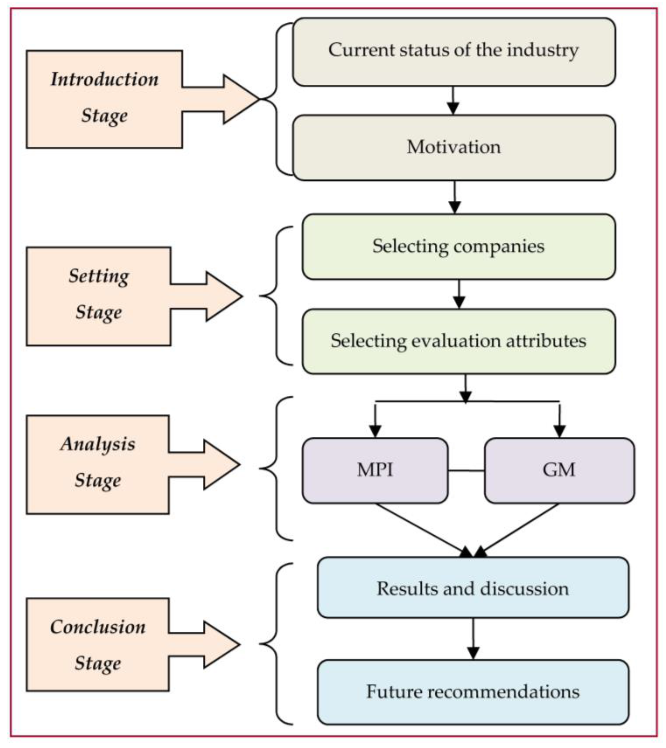
3. Research Procedure

In this research, a seven-step procedure is used, and the details of each step are described below and in Figure 1.

Step 1: Choose DMUs and collect their data: This step focuses on choosing DMUs in the Vietnam agroforestry industry and collecting their relevant information. The study investigates the relevant enterprises to find all potential candidates’ DMU lists. A total of 10 Vietnamese agroforestry companies with financial reports on the stock market during the period 2011–2014 are selected.

Step 2: Choose input/output variables: This step focuses on selecting the input and output variables. The selected input and output variables are critical, as they can affect the results. In this research, we refer to previous studies in order to make an appropriate choice. The Pearson correlation test will be used in Step 6 to check the suitability of these selected variables. However, according to the rule of thumb from Golany and Roll [11], the total DMUs need to be more or equal than double the number of inputs plus outputs.

Step 3: Grey prediction: In this step, the GM is used to predict the future data in 2015 and 2016. Since the prediction always exists with errors, the mean absolute percent error (MAPE) is used in the next step to check the prediction accuracy of the GM. Even though there are several prediction methodologies, almost all of them need to prepare lots of historical data. The GM is the only one that uses a minimum of four historical data types for prediction. The historical data are difficult to be collected in the Vietnamese agroforestry industry. Therefore, this study uses GM as a prediction method for overcoming a shortage of data.

Step 4: Check forecasting accuracy: As stated in the previous step, the MAPE is employed to check the prediction accuracy of the GM (1,1). Lewis [24] gave MAPE an assessment standard: a MAPE value < 10% is considered “good”; a MAPE value between 10%–20% is considered “qualified”; a MAPE value between 20%–50% is considered “just”; and a MAPE value > 50% is considered “unqualified”. If the forecasting error is too high, we have to go back to the Step 2 to reselect the input and output variables.

Step 5: Pearson correlation test: DEA requires the selected input and output variables to have an isotonic relationship. Therefore, to test that the data matches this isotonic prerequisite, the variable correlation analysis is calculated to verify a positive correlation between the selected inputs and outputs. If there are negative coefficient variables, the input and output variables need to be changed. Thus, we have to revert to the Step 2, until this prerequisite is met. In this research, we will employ the Pearson correlation test for this purpose.

Step 6: Choose the DEA model: This step includes many DEA models. Most of them can only analyze a single time period. However, only MPI can combine several time periods for integrated analysis and can separately discuss the changes of efficiency and technology. These characteristics match our data of several time periods and match our requirement of integrated analysis. Therefore, this study chooses a MPI model to assess and rank the efficiencies of DMUs for our analysis.

Step 7: Performance analysis: In this step, the forecasting performances of DMUs will be thoroughly analyzed.

4. Methodology

4.1. Grey Forecasting Model

Due to its popularity and computational efficiency, the GM (1,1) is used in this research for forecasting. The GM (1,1) is a type of time-series forecasting model with multiple inputs and outputs. One advantage of the GM (1,1) is that it does not need an entire set of historical data, but at least a set of four series data is required [18]. These series data have to be taken at equal intervals and bypassing any data in a sequential order is not allowed. The procedure of applying the GM (1,1) to forecasting is detailed as follows [25].

From the historical data we can derive the original time series dataset $X^{(0)}$, as shown in Equation (1):

$$X^{(0)}=(X^{(0)}(1),X^{(0)}(2),\mathrm{...},X^{(0)}(n)), n\ge 4$$

(1)

where $X^{(0)}$ is a non-negative sequence, and n is the total number of data observations.

From $X^{(0)}$, we can derive the accumulated time series data $X^{(1)}$, as shown in Equation (2):

$$X^{(1)}=(X^{(1)}(1),X^{(1)}(2),\mathrm{...},X^{(1)}(n)), n\ge 4$$

(2)

where:

$$X^{(1)}(1)=X^{(0)}(1)\mathrm{if}k=1$$

(3)

$$X^{(1)}(k)={\displaystyle \sum _{i=1}^k{X}^{(0)}(i)}\mathrm{if}k=2,\dots ,n$$

(4)

Then, the mean sequence $Z^{(1)}$ of $X^{(1)}$ can be derived as shown in Equation (5):

$$Z^{\left(1\right)}=\left(Z^{\left(1\right)}\left(2\right),Z^{\left(1\right)}\left(3\right),\dots ,Z^{\left(1\right)}\left(n\right)\right)$$

(5)

where Z⁽¹⁾(k) is the mean value of two adjacent data, i.e.,:

$$Z^{(1)}(k)=\frac{1}{2}\left(X^{(1)}(k)+X^{(1)}(k-1)\right), k=2,3,\mathrm{...},n$$

(6)

From $X^{(1)}$, a GM (1,1) model which corresponds to the first order differential equation $X^{(1)}\left(k\right)$ (Equation (7)) can be constructed as follows:

$$\frac{d{X}^{(1)}(k)}{dk}+a{X}^{(1)}(k)=b$$

(7)

where parameters a and b are called the developing coefficient and grey input, respectively.

In practice, the parameters a and b are not directly calculated from Equation (7); they are actually derived from Equation (8):

$${[a,b]}^T={(B^{T}B)}^{-1}{B}^{T}Y$$

(8)

where $Y=\left[\begin{array}{l}{X}^{(0)}(2)\\ X^{(0)}(3)\\ ...\\ ...\\ X^{(0)}(n)\end{array}\right]$ and $B=\left[\begin{array}{l}-Z^{(1)}(2)\begin{array}{c}1\end{array}\\ -Z^{(1)}(3)\begin{array}{c}1\end{array}\\ ...\begin{array}{c}⋮\end{array}\\ ...\begin{array}{c}⋮\end{array}\\ -Z^{(1)}(n)\begin{array}{c}1\end{array}\end{array}\right]$.

The vector Y is called the data series, vector B is called the data matrix, and ${[a,b]}^T$ is called the parameter series.

After substituting the derived values of a and b into Equation (9), this resulting equation can then be used to generate the accumulated time series values of prediction, which can be organized into a set of values as shown in Equation (10).

$${\hat{X}}^{(1)}(k+1)=\left[X^{(0)}(1)-\frac{b}{a}\right]e^{-ak}+\frac{b}{a}$$

(9)

where ${\hat{X}}^{(1)}(k+1)$ denotes the accumulated value of prediction of variable X at the time point k + 1.

$${\hat{X}}^{(1)}=({\hat{X}}^{(1)}(1),{\hat{X}}^{(1)}(2),...,{\hat{X}}^{(1)}(n))$$

(10)

where ${\hat{X}}^{(1)}(1)=X^{(0)}(1)$.

Substituting the k value (k = 1, …, n) into Equation (11) we can then find the set of forecasting values as shown in Equation (12):

$${\hat{X}}^{(0)}(k+1)=\left[X^{(0)}(1)-\frac{b}{a}\right]e^{-ak}(1-e^a)$$

(11)

$${\hat{X}}^{(0)}={\widehat{(X}}^{(0)}(1),{\hat{X}}^{(0)}(2),...,{\hat{X}}^{(0)}(n))$$

(12)

Errors always exist in forecasting, which can be classified into bias or random types. A bias error is a consistent result of mistakes—predicting too high or low. Such errors are often demand patterns being inaccurately estimated, such as trend, seasonal, or cyclic pattern results. Random errors are unpredictable factors. To understand the accuracy of forecasting models one needs to check the forecast errors. For this purpose the measurement, MAPE, is used. The equation of MAPE is defined in Equation (13), where n is the total number of data observations. A smaller MAPE means a higher forecasting accuracy.

$$\mathrm{MAPE}=\frac{\frac{{\displaystyle \sum \left|Actua{l}_t-Forecas{t}_t\right|}}{Actua{l}_t}\times 100}{n}$$

(13)

Lewis [24] gave an assessment standard for MAPE as follows: a MAPE value < 10% is considered “good”; a MAPE value between 10%–20% is considered “qualified”; a MAPE value between 20%–50% is considered “just”; a MAPE value > 50% is considered “unqualified”.

4.2. Malmquist Productivity Index

Caves et al. developed MPI in 1982 and the major DEA model for productivity measurement is MPI [26]. The MPI calculated the relative performance of a DMU in different periods of time using the technology of the base period [27]. The MPI is used to evaluate the change in efficiency of a DMU between two time periods [28]:

$$\mathrm{MPI}={\left[\frac{d_o^s(x_t,y_t)}{d_o^s(x_s,y_s)}\times \frac{d_o^t(x_t,y_t)}{d_o^t(x_s,y_s)}\right]}^{1/2}$$

(14)

where $d_o^s$ is a distance function measuring the efficiency of the conversion of inputs x_s to outputs y_s in the period s (note that DEA efficiency is considered a distance measure in the literature as it reflects the efficiency of converting inputs to outputs).

Importantly, if there is a technological change in period t, then, $d_o^t(x_s,y_s)=\mathrm{Efficiency}\mathrm{of}\mathrm{conversion}\mathrm{of}\mathrm{input}\mathrm{in}\mathrm{period}\mathrm{s}\mathrm{to}\mathrm{output}\mathrm{in}\mathrm{period}s\ne d_o^s(x_s,y_s)$.

MPI considers two-period efficiency and technological change in the geometric mean. MPI was defined in Equation (15) and was being used to estimate the change of overall productivity of a pharmaceutical company over time. If MPI > 1 it means overall productivity increases; if MPI = 1 it indicates no change; a MPI < 1, it indicates a decrease of overall productivity:

$$\mathrm{MPI}=\frac{d_o^t(x_t,y_t)}{d_o^s(x_s,y_s)}{\left[\frac{d_o^s(x_s,y_s)}{d_o^t(x_s,y_s)}\times \frac{d_o^s(x_t,y_t)}{d_o^s(x_t,y_t)}\right]}^{1/2}=\mathrm{Efficiency}\mathrm{change}\times \mathrm{Technological}\mathrm{change}$$

(15)

The “efficiency change” is also called the “catch-up” effect, indicating the extent that a DMU improves or deteriorates its efficiency. If the change in efficiency > 1 then it represents relative efficiency progress from time period s to t; if change in efficiency = 1 or < 1 it indicates there is no change or recession, respectively. The “technological change” is also called the “frontier shift effect” (or innovative effect), reflecting the frontier change between the two periods. If technological change > 1 it represents technological progression; technological change < 1 shows technological recession.

5. Empirical Results

Following the research procedure proposed in Section 3,

Table 1. The list of 10 DMUs selected from Vietnam agroforestry industry.

Number Order	DMU	Company Name	Stock Market Code
1	DMU1	Dong Phu Rubber Joint Stock Company	HOSE: DPR
2	DMU2	HAGL Joint Stock Company	HOSE: HAG
3	DMU3	Hoa Binh Rubber Joint Stock Company	HOSE: HRC
4	DMU4	National Seed Joint Stock Company	HOSE: NSC
5	DMU5	Phuoc Hoa Rubber Joint Stock Company	HOSE: PHR
6	DMU6	Southern Seed Corporation	HOSE: SSC
7	DMU7	Thong Nhat Rubber Joint Stock Company	HOSE: TNC
8	DMU8	Tay Ninh Rubber Joint Stock Company	HOSE: TRC
9	DMU9	Quang Nam Rubber Investment JSC	HOSE: VHG
10	DMU10	Vinacafe Son Thanh Joint Stock Company	OTC: AUM

shows 10 Vietnamese agroforestry companies selected for this research. These companies are the top companies in the agroforestry industry in Vietnam, and their data are posted publicly and prestigiously. These companies are qualified with transparent financial data. Information about these DMUs was collected from the market observation posting system of Vietstock.vn, which is a premier site for business and financial market news in Vietnam.

Referring to the literature review, this research selects total assets, liabilities, and equity as the three inputs factors, and net revenue and gross profit as the output factors. The total has 10 DMUs with three inputs and two outputs. Matching the rule of thumb from Golany and Roll [11], which states that the total number of DMUs need to be more or equal than double the number of inputs plus outputs. The correlation of these selected input and output variables will be validated by the Pearson correlation test.

Having determined these input and output variables, we collect the historical data of these DMUs from 2011 to 2014 [6,29]. However, due to space limitations, only the data of the year 2014 are listed in

Table 2. Inputs and outputs data of DMU_s in 2014.

DMUs	Inputs ( Millions of VND)			Outputs (Millions of VND)
	(I) Total Asset	(I) Liabilities	(I) Equity	(O) Net Revenue	(O) Gross Profit
DMU1	3,312,062	658,039	2,195,471	938,682	285,480
DMU2	36,368,864	20,978,624	14,237,728	3,054,331	1,226,993
DMU3	686,336	181,918	504,418	161,394	7059
DMU4	953,008	202,337	744,946	719,136	287,323
DMU5	3,428,830	1,129,528	2,253,082	1,604,981	275,288
DMU6	537,355	162,978	373,160	608,625	190,717
DMU7	332,605	30,901	301,704	63,873	−355
DMU8	1,587,255	140,308	1,446,947	500,638	121,259
DMU9	1,071,970	126,832	900,392	394,873	46,077
DMU10	13,283	2675	10,608	21,611	158

.

Following the research procedure, the GM (1,1) is used in this section to predict the future data from 2015 and 2016 for the selected DMUs.

Table 3. The historical data (2011–2014) of the input and output variables of DMU₁.

DMU1	Inputs (Millions of VND)			Outputs (Millions of VND)
	(I) Total Asset	(I) Liabilities	(I) Equity	(O) Net Revenue	(O) Gross Profit
2011	2,430,078	491,056	1,910,113	1,837,202	866,224
2012	2,821,172	556,960	2,179,990	1,376,951	553,307
2013	3,328,252	606,600	2,298,599	1,100,122	424,953
2014	3,312,062	658,039	2,195,471	938,682	285,480

shows the DMU₁’s historical data (2011–2014) used by the GM (1,1).

Below, we use the “total asset data” of DMU₁ in Table 3 to illustrate the generation of the forecasting data of DMU₁ step-by-step.

(1)

Create the primitive series

$$X^{\left(0\right)}=\left(2,430,078,2,821,172,3,328,252,3,312,062\right)$$

(2)

Generate the accumulated series $X^{(1)}$

$$X^{\left(1\right)}=\left(2,430,078,5,251,250,8,579,502,11,891,564\right)$$

Where

$$\begin{gathered} X^{(1)}(1)=X^{(0)}(1)=2,430,078 \\ {X}^{(1)}(2)=X^{(0)}(1)+X^{\left(0\right)}(2)=5,251,250 \\ {X}^{(1)}(3)=X^{(0)}(1)+X^{\left(0\right)}(2)+X^{(0)}(3)=8,579,502 \\ {X}^{(1)}(4)=X^{(0)}(1)+X^{\left(0\right)}(2)+X^{(0)}(3)+X^{(0)}(4)=11,891,564 \end{gathered}$$

(3)

Create mean series dataset $Z^{(1)}$

To find the mean series dataset $Z^{(1)}$, Equation (6) is used and we derive the following data.

$$\begin{gathered} X^{(1)}(1)=X^{(0)}(1)=2,430,078 \\ {Z}^{(1)}(2)=\frac{1}{2}(2,430,078+5,251,250)=3,840,664 \\ {Z}^{(1)}(3)=\frac{1}{2}(5,251,250+8,579,502)=6,915,376 \\ {Z}^{(1)}(4)=\frac{1}{2}(8,579,502+11,891,564)=10,235,533 \end{gathered}$$

Then, $Z^{(1)}=(Z^{(1)}(2),Z^{(1)}(3),Z^{(1)}(4))=\left(3,840,660,6,915,376,10,235,533\right).$

(4)

Find the values for coefficients a and b

Let $B=\left[\begin{array}{c}-3,840,664\\ -6,915,376\\ -10,235,533\end{array}\begin{array}{c}1\\ 1\\ 1\end{array}\right]$, $\hat{\theta }=\left[\begin{array}{c}a\\ b\end{array}\right]$, $y_N=\left[\begin{array}{c}2,821,172\\ 3,328,252\\ 3,312,062\end{array}\right]$.

Then, using the Equation (8), we can derived the values of a and b as below.

$$\left[\begin{array}{c}a\\ b\end{array}\right]=\hat{\theta }={(B^{T}B)}^{-1}{B}^T{y}_N=\left[\begin{array}{c}-0.0756791\\ 2,624,287.78\end{array}\right]$$

(5)

Generate the accumulated data series

Substitute the two coefficients a and b, as well as the k values (k = 0, …, 7), into the Equation (9); then we can derive the accumulated data series in the third column in

Table 4. The derived prediction values X(k).

k	X(k)	Value	X(k)	Value
k = 0	X(1)	2,430,078	X(1)	2,430,078
k = 1	X(2)	5,347,264.63	X(2)	2,917,186.63
k = 2	X(3)	8,493,789.83	X(3)	3,146,525.2
k = 3	X(4)	11,887,683.4	X(4)	3,393,893.54
k = 4	X(5)	15,548,392.5	X(5)	3,660,709.08
k = 5	X(6)	19,496,893.1	X(6)	3,948,500.68
k = 6	X(7)	23,755,810.6	X(7)	4,258,917.41
k = 7	X(8)	28,349,548.5	X(8)	4,593,737.97

.

(6)

Generate the series values of prediction

Substitute the two coefficients a and b, as well as the k values (k = 0, …, 7) into the Equation (11); then we can the derive the fifth column in Table 4.

With the same computational process, the study could obtain the forecasting data of all DMUs in 2015 and 2016, as shown in

Table 5. Predicted input and output data of all DMU_s in 2015 and 2016.

Year	DMUs	Inputs (Currency Unit: Millions of VND)			Outputs (Currency Unit: Millions of VND)
		(I) Total Asset	(I) Liabilities	(I) Equity	(O) Net Revenue	(O) Gross Profit
2015	DMU1	3,660,709.08	715,051.35	2,239,955.23	759,042.36	216,764.72
	DMU2	38,126,475.9	19,810,053.2	17,301,061.4	2,169,114.51	1,234,682.16
	DMU3	710,528.52	192,011.93	518,491.25	140,856.83	2963.25
	DMU4	1,427,295.43	256,101.60	1,160,150.10	816,038.05	343,084.35
	DMU5	3,646,880.39	1,210,168.95	2,382,125.12	1,369,690.16	209,289.74
	DMU6	601,752.38	169,376.87	436,089.19	715,599.93	213,766.23
	DMU7	308,391.58	21,024.41	288,886.80	49,637.40	1344.39
	DMU8	1,765,695.56	259,012.54	1,529,264.81	370,704.24	80,840.40
	DMU9	1,534,558.85	108,114.20	1,366,325.23	584,979.71	43,400.28
	DMU10	13,221.75	2551.08	10,749.15	24,795.80	177.04
2016	DMU1	3,948,500.68	777,109.40	2,247,634.11	624,477.72	158,370.95
	DMU2	41,364,890.23	20,100,095.76	20,670,001.67	1,748,357.56	1,248,329.47
	DMU3	725,873.82	196,885.59	528,955.14	91,601.17	1261.76
	DMU4	2,418,284.18	349,367.53	2,116,736.15	939,274.77	412,839.94
	DMU5	3,829,240.64	1,250,205.83	2,512,384.37	1,167,365.28	142,525.83
	DMU6	678,367.07	173,410.58	517,540.57	813,804.44	242,919.54
	DMU7	288,308.59	15,960.23	276,386.25	31,491.09	398.52
	DMU8	1,816,554.47	248,283.06	1,606,736.41	275,684.53	52,543.82
	DMU9	2,386,716.78	101,837.68	2,318,982.81	971,069.14	138,457.14
	DMU10	12,975.19	2287.63	10,853.25	29,651.57	109.37

.

In this step we check the prediction accuracy of the GM (1,1) based on the MAPE values. When a MAPE value is small it means the predicted value is close to the actual value. The MAPE values obtained are shown in

Table 6. Average MAPE errors of DMU_s.

DMUs	MAPE	DMUs	MAPE
DMU1	1.626%	DMU6	7.792%
DMU2	5.663%	DMU7	2.069%
DMU3	2.256%	DMU8	1.124%
DMU4	4.001%	DMU9	14.513%
DMU5	5.021%	DMU10	7.046%
Average MAPE: 5.111%

.

As the MAPE values obtained are, mostly, smaller than 10%, especially as the average MAPE of the 10 DMUs reaches 5.111% (below 10%, as well), it confirms that the GM (1,1) provides a good prediction accuracy in this research.

However, before using this DEA model, we have to ensure that input and output variables have isotonic relationships. This means that if the input quantity increases, then the output quantity could not decrease under the same condition. Thus, a Pearson correlation test is first used to ensure this prerequisite. A higher correlation coefficient refers to a closer relationship between two variables, and a low correlation coefficient means a low relationship. The interpretation of the correlation coefficient is explained in more detail as follows: The correlation coefficient is always between −1 and +1. When the correlation coefficient is closer to ± 1, this means two groups are closer to a perfect linear relationship. When a correlation value is less than 0.2 then the degree of correlation is considered “very low”; a value between 0.4–0.6 is considered “average high”; a value between 0.6–0.8 is considered “efficient high”; a value between 0.8–1 is considered “upper high”. Our empirical results (

Table 7. The correlations between input and output variables in 2011–2016.

2011	Total Asset	Liabilities	Equity	Net Revenue	Gross Profit
Total asset	1	0.997951	0.993387	0.755161	0.781175
Liabilities	0.997951	1	0.98401	0.719137	0.744403
Equity	0.993387	0.98401	1	0.81337	0.840045
Net Revenue	0.755161	0.719137	0.81337	1	0.99058
Gross profit	0.781175	0.744403	0.840045	0.99058	1
2012	Total Asset	Liabilities	Equity	Net Revenue	Gross Profit
Total asset	1	0.997593	0.987721	0.916987	0.865799
Liabilities	0.997593	1	0.97452	0.892273	0.832981
Equity	0.987721	0.97452	1	0.957569	0.924983
Net Revenue	0.916987	0.892273	0.957569	1	0.983508
Gross profit	0.865799	0.832981	0.924983	0.983508	1
2013	Total Asset	Liabilities	Equity	Net Revenue	Gross Profit
Total asset	1	0.997283	0.997084	0.847284	0.927948
Liabilities	0.997283	1	0.988945	0.821053	0.90642
Equity	0.997084	0.988945	1	0.874179	0.946157
Net Revenue	0.847284	0.821053	0.874179	1	0.967438
Gross profit	0.927948	0.90642	0.946157	0.967438	1
2014	Total Asset	Liabilities	Equity	Net Revenue	Gross Profit
Total asset	1	0.998139	0.99682	0.901523	0.964055
Liabilities	0.998139	1	0.990301	0.88317	0.955216
Equity	0.99682	0.990301	1	0.923212	0.970017
Net Revenue	0.901523	0.88317	0.923212	1	0.956117
Gross profit	0.964055	0.955216	0.970017	0.956117	1
2015	Total Asset	Liabilities	Equity	Net Revenue	Gross Profit
Total asset	1	0.998182	0.998555	0.829165	0.960343
Liabilities	0.998182	1	0.993988	0.810135	0.955803
Equity	0.998555	0.993988	1	0.846913	0.961551
Net Revenue	0.829165	0.810135	0.846913	1	0.895381
Gross profit	0.960343	0.955803	0.961551	0.895381	1
2016	Total Asset	Liabilities	Equity	Net Revenue	Gross Profit
Total asset	1	0.997754	0.998123	0.722542	0.95035
Liabilities	0.997754	1	0.992805	0.693972	0.94331
Equity	0.998123	0.992805	1	0.749176	0.955682
Net Revenue	0.722542	0.693972	0.749176	1	0.818206
Gross profit	0.95035	0.94331	0.955682	0.818206	1

) indicate that these variables have strong positive correlations, indicating that these selected input and output factors are qualified.

Though some DEA models are available for assessing DMUs, the efficiencies of DMUs of several time periods cannot be compared for most of the DEA models [30]. In this research, the Malmquist model is used to evaluate the performances of DMUs.

Table 8. The catch up, frontier, and MPI of DMUs from 2011 to 2016.

	Catch-up
DMUs	2011–2012	2012–2013	2013–2014	2014–2015	2015–2016	Average
DMU1	0.829064	1.017534	0.481122	0.480225	0.588611	0.679311
DMU2	1	1	1	1	1	1
DMU3	0.507493	0.750196	0.49117	0.769674	0.560938	0.615894
DMU4	1.50032	1.511764	1.219231	1.639257	0.924659	1.359046
DMU5	0.734399	1.295857	0.878322	1.130413	0.69098	0.945994
DMU6	0.654229	1.36234	1.36408	1.353088	1.36118	1.218983
DMU7	0.464872	0.938184	0.522882	0.827553	0.431461	0.63699
DMU8	1.311197	0.251778	1.519396	0.453193	0.694019	0.845917
DMU9	0.642412	1.125074	1.68504	2.313033	2.063988	1.565909
DMU10	1.146358	0.860033	1.023463	0.897824	0.935341	0.972604
	Frontier
DMUs	2011–2012	2012–2013	2013–2014	2014–2015	2015–2016	Average
DMU1	0.294275	0.492147	0.572874	1.042527	1.166415	0.713647
DMU2	1	1.046866	0.925847	1	1	0.994543
DMU3	1.069373	1.016991	0.825623	1.08088	1.072451	1.013064
DMU4	0.883812	0.963577	0.776533	1.286913	1.603398	1.102847
DMU5	0.402361	0.358968	0.521382	0.392711	0.455877	0.42626
DMU6	1.107621	1.001566	0.74005	1.023985	1.10437	0.995519
DMU7	1.037761	1.067316	0.643354	1.156675	1.334136	1.047848
DMU8	0.730453	0.954731	0.791898	1.093495	1.05964	0.926043
DMU9	1.115798	1.024782	0.796385	1.072349	1.343707	1.070604
DMU10	1.063773	1.049261	1.178219	1.181882	1.223364	1.1393
	MPI
DMUs	2011–2012	2012–2013	2013–2014	2014–2015	2015–2016	Average
DMU1	0.243973	0.500777	0.275622	0.500648	0.686564	0.441517
DMU2	1	1.046866	0.925847	1	1	0.994543
DMU3	0.542699	0.762943	0.405521	0.831925	0.601579	0.628934
DMU4	1.326001	1.456701	0.946773	2.109581	1.482596	1.464331
DMU5	0.295494	0.465171	0.457941	0.443925	0.315002	0.395506
DMU6	0.724637	1.364473	1.009488	1.385542	1.503246	1.197477
DMU7	0.482426	1.001338	0.336398	0.957209	0.575628	0.6706
DMU8	0.957768	0.24038	1.203207	0.495564	0.73541	0.726466
DMU9	0.716802	1.152955	1.34194	2.480379	2.773395	1.693094
DMU10	1.219464	0.902399	1.205864	1.061122	1.144262	1.106622

shows the results derived from the Malmquist O-V model. To facilitate the analysis, the values of efficiency change, technological change, and MPI are depicted in Figure 2, Figure 3 and Figure 4, respectively.

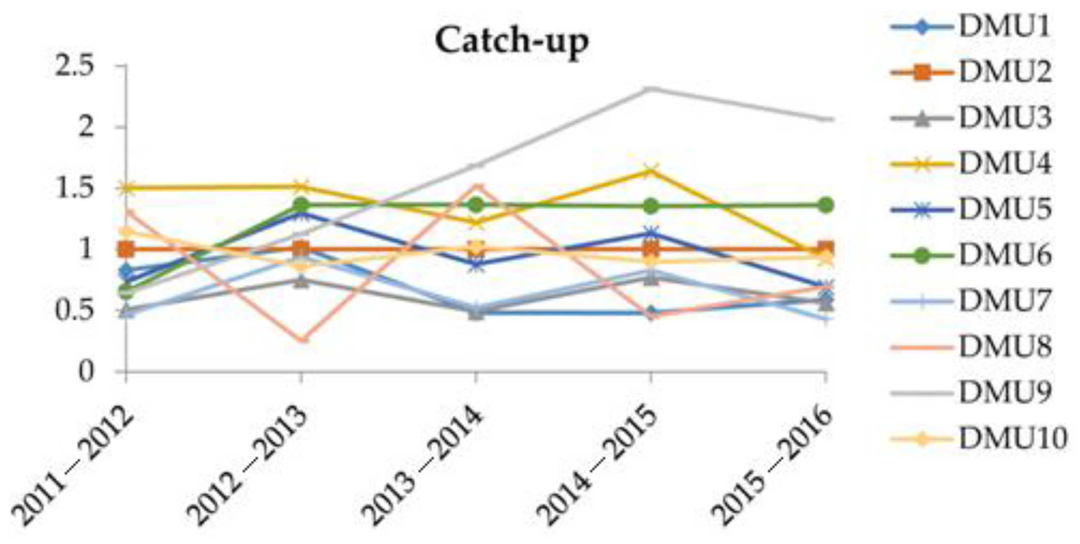
Figure 2 shows the “efficiency changes” (catch-up effects) of the 10 DMUs over the time period 2011–2016. It is found that the efficiency changes of these DMUs fluctuated over these years, especially DMU₃, DMU₄, and DMU₈. DMU₃ had experienced a dramatic efficiency rise during the time period 2011–2015, and DMU₄ experienced a dramatic efficiency drop during the time period 2015–2016, while the DMU₈ had experienced a dramatic drop during the time period 2014–2015. Except for DMU₂ and DMU₆, which had experienced slight efficiency changes, the other DMUs all had experienced some degree of efficiency fluctuations. In terms of “efficiency change”, DMU₉, DMU₄, and DMU₆ are the top three best companies, while the top three worst companies are DMU₃, DMU₇, and DMU₁. DMU₂ is found with a stable efficiency, but it also had not improved its efficiency in the current and near future. From Figure 2, we can determine and predict the efficiency changes, or the “catch-up” effects, of each DMU.

Figure 3 show the “technological changes” (frontier-shift) of the 10 DMUs from 2011–2016. It is found that, except for DMU₅, other DMUs had experienced an upward technological change, though most of them had experienced an efficiency drop during 2013–2014. This implies most of these DMUs had continued to improve their technological capabilities. DMU₅ always keeps a lower “technological changes” score, indicating that it has not actively improved its technology. Thus, DMU₅ requires further investigation into the causes that lead to its tardiness on technology development. In terms of “technological change”, DMU₁₀, DMU₄, and DMU₉ are the top three best companies, while the top three worst companies are DMU₅, DMU₁, and DMU₈.

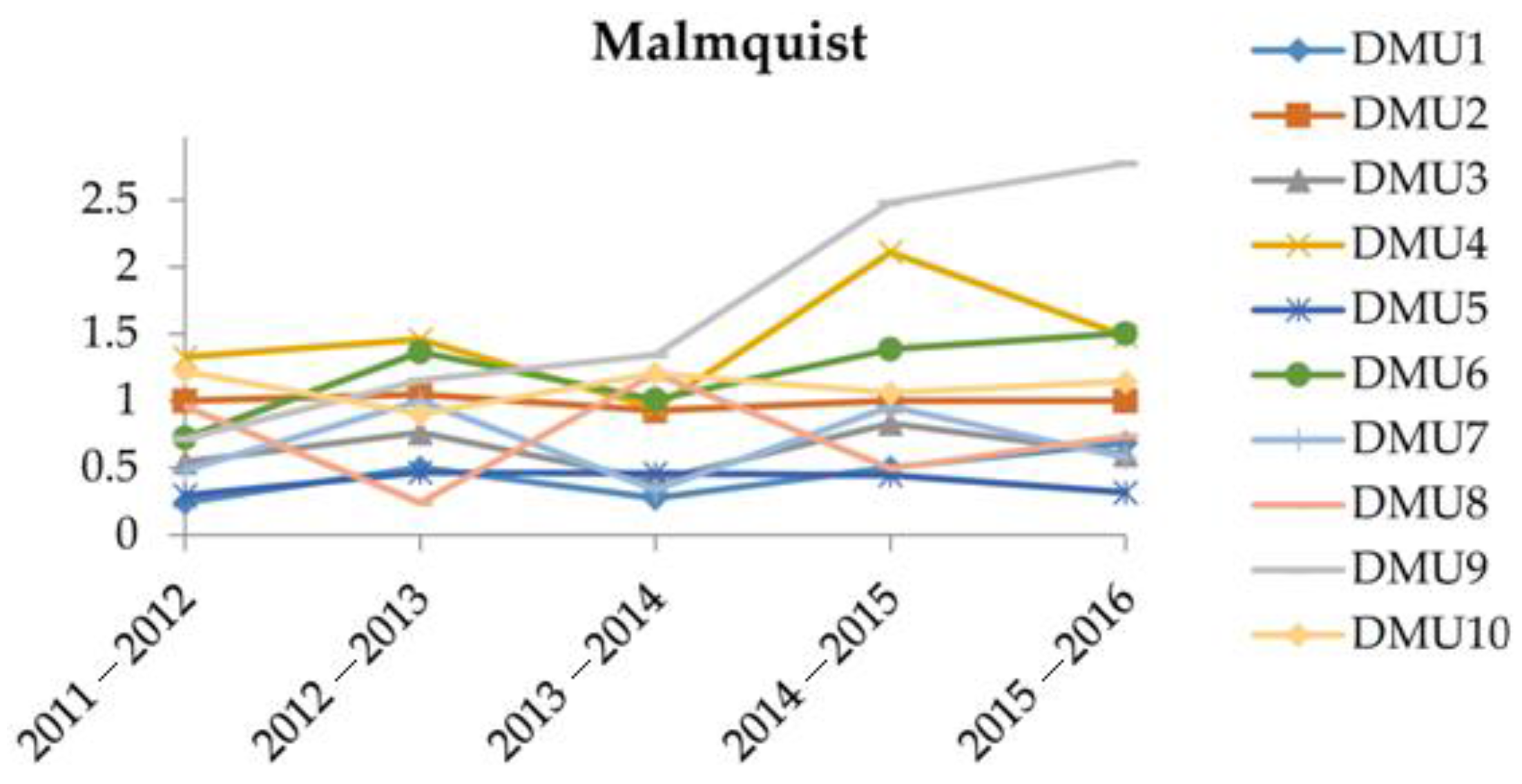
Figure 4 shows the MPI, the total productivity of the 10 DMUs from 2011–2016. It is noted that DMU₆ and DMU₉ had a long-term upward trend during 2011–2016, though DMU₆ had experienced a drop during 2013–2014. In terms of MPI, DMU₉, DMU₄, and DMU₁₀ are the top three best companies, while the top three worst companies are DMU₅, DMU₁, and DMU₇. DMU₈ appears unstable due to having the largest fluctuation; thus, it requires intense care for its development. In summary, to sustain the development of the agroforestry industry, the Vietnamese government needs to especially focus on DMU₅, DMU₁, DMU₇, and DMU₈.

6. Conclusions

For sustainable development of the Vietnamese agroforestry industry, this research has proposed a hybrid approach combining GM and DEA to assess the current, and predict the future, performance of agroforestry companies. This study first selects total assets, liabilities, and equity as input variables, and net revenue and gross profit as output variables. After collecting the historical data (2011–2014) from the Vietnam stock market, the GM (1,1) model is used to forecast the future data in 2015–2016 for selected agroforestry enterprises. The MAPE value of 5.11% confirms the desired accuracy of the GM (1,1). Based on the historical and predicted data, the Malmquist model is used to assess the performance of these DMUs. The derived results provide insight views into the agroforestry companies in terms of “efficiency changes”, “technological changes”, and MPI (total productivity). These results can also provide insight into the “past-current-future” performances of these DMUs. In summary, to sustain the development of Vietnamese agroforestry industry, the government should take more care in the developments of these companies, which are DMU₅, DMU₁, DMU₇, and DMU₈.

This research also demonstrates that the proposed approach can help decision-makers. Policy-makers can use the approach to develop strategies to sustain the development of the Vietnamese agroforestry industry. Investors can use of this approach to discover the good companies for investments. This mathematical approach reduces the errors and risks in decision-making. In addition, the approach can be used in other industries to extend its contributions. This study provides many significant and noticeable results. This numerical study gives us better “past-present-future” insights through the integration method, and this work could be used as a better model for performance analysis among the decision-makers of varied industries.

The proposed approach has been applied to the Vietnamese agroforestry industry; however, it only includes 10 companies listed on the stock market. Including more companies can provide further focus. In addition, some other input and output variables (such as the number of staff, number of branches, revenue, research and development, etc.) can be taken to measure the performance of these companies. Moreover, different DEA models can be further investigated for comparisons. Furthermore, this approach can be applied to other industries.

References

1. Torquebiau, E.F. A renewed perspective on agroforestry concepts and classification. C. R. Acad. Sci. 2000, 323, 11009–11017. [Google Scholar] [CrossRef]
2. DeWit, R.; Leibreich, J.; Vernier, F.; Delmas, F.; Beuffe, H.; Maison, P.; Capdeville, P. Relationship between land-use in the agro-forestry system of les Landes, nitrogen loading to and risk of macro-algal blooming in the Bassin d’Arcachon coastal lagoon (SW France). Estuar. Coast. Shelf Sci. 2005, 62, 353–465. [Google Scholar]
3. Hurni, H.; Nuntapong, S. Agro-forestry improvements for shifting cultivation systems: Soil conservation research in northern Thailand. Mount. Res. Dev. 1983, 3, 338–345. [Google Scholar] [CrossRef]
4. Sharma, V.P.; Kumar, A. Factors influencing adoption of agro-forestry programme: A case study from North-West India. Indian J. Agric. Econ. 2000, 55, 300–510. [Google Scholar]
5. Craswell, E.T.; Sajjapongse, A.; Howlett, D.J.B.; Dowling, A.J. Agroforestry in the management of sloping lands in Asia and the Pacific. Agrofor. Syst. 1997, 38, 121–137. [Google Scholar] [CrossRef]
6. Annual Report, Vietnamese Minister of Industry and Trade. Available online: http://www.moit.gov.vn/en/Pages/default.aspx (accessed on 15 January 2016).
7. Fritzen, S. Growth, inequality and the future of poverty reduction in Vietnam. J. Asian Econ. 2002, 13, 635–657. [Google Scholar] [CrossRef]
8. Wang, C.N.; Nguyen, N.T.; Tran, T.T. Integrated DEA models and grey system theory to evaluate past-to-future performance: A case of Indian electricity industry. Sci. World J. 2015, 2015, 1–17. [Google Scholar] [CrossRef] [PubMed]
9. Wang, C.N.; Nguyen, X.T.; Wag, Y.H. Automobile industry strategic alliance partner selection: The application of a hybrid DEA and Grey theory model. Sustainability 2016, 8, 273. [Google Scholar] [CrossRef]
10. Charnes, A.; Cooper, W.W.; Rhodes, E. Measuring the efficiency of decision making units. Eur. J. Oper. Res. 1978, 2, 429–444. [Google Scholar] [CrossRef]
11. Golany, B.; Roll, Y. An application procedure for DEA. Omega 1989, 17, 237–250. [Google Scholar] [CrossRef]
12. Liu, S.T. Measuring and categorizing technical efficiency and productivity change of commercial banks in Taiwan. Expert Syst. Appl. 2010, 37, 2783–2789. [Google Scholar] [CrossRef]
13. Romano, G.; Guerrini, A. Measuring and comparing the efficiency of water utility companies: A data envelopment analysis approach. Util. Policy 2011, 19, 202–209. [Google Scholar] [CrossRef]
14. Briec, W.; Peypoch, N.; Ratsimbanierana, H. Productivity growth and biased technological change in hydroelectric dams. Energy Econ. 2011, 33, 853–858. [Google Scholar] [CrossRef]
15. Yang, H.; Yuan, T.; Zhang, X.; Li, S. A decade trend of total factor productivity of key state-owned forestry enterprises in China. Forests 2016, 7, 57. [Google Scholar] [CrossRef]
16. Qazi, A.Q.; Yulin, Z. Productivity measurement of hi-tech industry of China malmquist productivity index–DEA approach. Procedia Econ. Financ. 2012, 1, 330–336. [Google Scholar] [CrossRef]
17. Deng, J.L. Control problems of grey systems. Syst. Control Lett. 1982, 1, 288–294. [Google Scholar]
18. Deng, J.L. Introduction to grey system theory. J. Grey Syst. 1989, 1, 1–24. [Google Scholar]
19. Ren, J.; Gao, S.; Tan, S.; Dong, L. Prediction of the yield of biohydrogen under scanty data conditions based on GM (1,N). Int. J. Hydrog. Energy 2013, 38, 13198–13203. [Google Scholar] [CrossRef]
20. Kuo, Y.; Yang, T.; Huang, G.W. The use of grey relational analysis in solving multiple attribute decision-making problems. Comput. Ind. Eng. 2008, 55, 80–93. [Google Scholar] [CrossRef]
21. Lin, Y.H.; Wang, J.S.; Pai, P.F. A grey prediction model with factor analysis technique. J. Chin. Inst. Ind. Eng. 2004, 21, 535–542. [Google Scholar] [CrossRef]
22. Chen, Y.S.; Chen, B.Y. Applying DEA, MPI, and grey model to explore the operation performance of the Taiwanese wafer fabrication industry. Technol. Forecast. Soc. Chang. 2011, 78, 536–546. [Google Scholar] [CrossRef]
23. Wang, C.N.; Lin, L.C.; Murugesan, D. Analyzing PSU’s performance: A case from ministry of petroleum and natural gas of India. Math. Probl. Eng. 2013, 2013, 802690. [Google Scholar] [CrossRef]
24. Lewis, C.D. International and Business Forecasting Methods; Butterworths: London, UK, 1982. [Google Scholar]
25. Liu, S.; Forrest, J.Y.L. Grey Systems: Theory and Applications; Springer: Chennai, India, 2010. [Google Scholar]
26. Caves, D.W.; Christensen, L.R.; Diewert, W.E. The economic theory of index numbers and the measurement of input, output, and productivity. Econometrica 1982, 50, 1393–1414. [Google Scholar] [CrossRef]
27. Färe, R.; Grosskopf, S.; Norris, M.; Zhang, Z. Productivity growth, technical progress, and efficiency change in industrialized countries. Am. Econ. Rev. 1994, 84, 66–83. [Google Scholar]
28. Chen, Y. A non-radial Malmquist productivity index with an illustrative application to Chinese major industries. Int. J. Prod. Econ. 2003, 83, 27–35. [Google Scholar] [CrossRef]
29. Vietstock. Available online: http://vietstock.vn/ (accessed on 15 January 2016).
30. Banker, R.D.; Charnes, A.; Cooper, W.W. Some models for estimating technological and scale inefficiencies in data envelopment analysis. Manag. Sci. 1984, 30, 1078–1092. [Google Scholar] [CrossRef]
Figure 1. Research development flow.
Sustainability 08 01139 g001
Figure 2. Efficiency change or catch-up (2011–2016).
Sustainability 08 01139 g002
Figure 3. Technological change or Frontier shift (2011–2016).
Sustainability 08 01139 g003
Figure 4. MPI scores (2011–2016).
Sustainability 08 01139 g004