Groundwater Depth Prediction Using Data-Driven Models with the Assistance of Gamma Test

Abstract

Prediction of the groundwater dynamics via models can help better manage the groundwater resources and guarantee their sustainable use. Three types of data-driven models are built for groundwater depth prediction in the plain of Shijiazhuang, the capital of Hebei Province in North China. The data-driven models include the Power Function Model (PFM), Back-Propagation Artificial Neural Network (BPANN) and Support Vector Machines (SVM) with two kernel functions of linear kernel function (LKF) and radial basis function (RBF). Five classes of factors (including 12 indices) are considered as potential model input variables. The Gamma Test (GT) is adopted in this study to help identify the relative importance of the input indices and tackle the tricky issue of the optimal input combinations for the data-driven models. The established models are evaluated in both fitting and testing procedures based on the root mean squared error (RMSE) and Nash-Sutcliffe efficiency (E) for different input combination schemes. The results show that SVM (RBF) performs the best. It is interesting to find that the natural factors (i.e., precipitation and evaporation) are less relevant to the groundwater depth variations. The methods used in this study have much significance for groundwater depth prediction in areas lacking hydrogeological data.

1. Introduction

Groundwater is an important part of water resources for domestic, agricultural, industrial, and environmental uses due to its generally good quality, widespread availability, good water stability and the fact it is not easily polluted [1]. Groundwater resources are especially important in the arid and semi-arid regions, which can cover the shortage of water caused by uneven distribution of the surface water in time and space. However, arable land increases, urban expansion and population growth have caused a dramatic increase in water consumption, which has led to a decrease of the groundwater level in many countries all over the world [2,3].

With the rapid economic development in China in the past several decades, the demand for water has increased at a fast speed. This has led to an excessive use of water resources, especially groundwater. At present, there are many groundwater overdraft areas in China, among which Hebei Province in North China plain is one of the most serious overdraft areas where the groundwater level has decreased dramatically [4,5]. Much attention has been paid by both researchers and policy makers in this area. There have been studies focusing on both the reasons for and the negative effects of the continuous decline of the groundwater level in Hebei province and the North China plain [6,7].

Groundwater dynamic forecasting provides important information for groundwater management. Physical descriptive models and data-driven models are two classes of dynamic prediction models [8]. Detailed hydrogeological data in space and time, which are usually obtained by a large number of field experiments, are required to construct the physical models in practical application. So, a data-driven model is a good choice when data are limited and the groundwater system is complex. Power Function Model (PFM), Back-Propagation Artificial Neural Network (BPANN) and Support Vector Machines (SVM) are popular data-driven models used for forecasting the groundwater level [9,10,11]. Among these methods, PFM is a simple non-linear regression (NLR) model, while the other two models are more complex. Some studies indicate that the BPANN model and SVM model perform better, especially the SVM model [12], but the prediction abilities of these two models are not always good for all cases due to the complexities of hydrogeological conditions and the groundwater flow in different regions [13].

There are many causes for the decrease of the groundwater level, including natural factors, anthropic factors, biological factors and economic factors, which can all be treated as the inputs of the data-driven models. To construct a reliable data-driven model for groundwater prediction, some challenging questions need to be answered beforehand. For example, which inputs are relevant to the groundwater level and which are irrelevant? To what extent do the inputs determine the output from a smooth model? How many data points are required to make a prediction with the best possible accuracy? So far, these questions have not been addressed adequately in groundwater level prediction using data-driven models. However, it is possible that significant progress can be made to tackle these questions, because the Gamma Test (GT) has been presented as an efficient algorithm. By estimating the variance of the noise in the raw data, GT can directly estimate the best mean squared error for a given selection of input by a smooth model on unseen data, before the model construction. In this way, it can help find the best input data combination and identify the sufficient number of data points used for model training. A formal proof of the GT can be found in Evans and Jones [14]. Then, a series of studies have indicated that GT can greatly reduce the model construction work and can potentially be used in the area of hydrological prediction and water management. Moghaddamnia and colleagues used GT to select the input data for Artificial Neural Networks (ANN) and the adaptive neuro-fuzzy inference system for evaporation estimation [15]. Noori and colleagues assessed the SVM model performance for monthly stream flow prediction with the assistance of GT [16]. Han and colleagues explored the model structure for index flood regionalization using GT [17]. However, with respect to groundwater prediction, little work has been done using this efficient tool.

In this study, GT is used to rank the relative importance of the model inputs and find the best input combinations before the data-driven models are calibrated. Three data-driven models, i.e., PFM, BPANN and SVM, are used to predict the variations of the groundwater depth and the performances of the three established models are further compared. Twelve indices, including natural, anthropic, biological, economic and social factors which may influence the groundwater depth, are considered as the input of the data-driven models. The study is carried out in the plain of Shijiazhuang, the capital city of Hebei province in North China. During the past three decades, the groundwater level in this region has declined by 30 m, which has not only restricted the development of the economy but has also caused serious environmental problems [18]. It is hoped that the study can provide a novel and complementary methodology for the prediction of groundwater level dynamics in the study area.

2. Data and Methodology

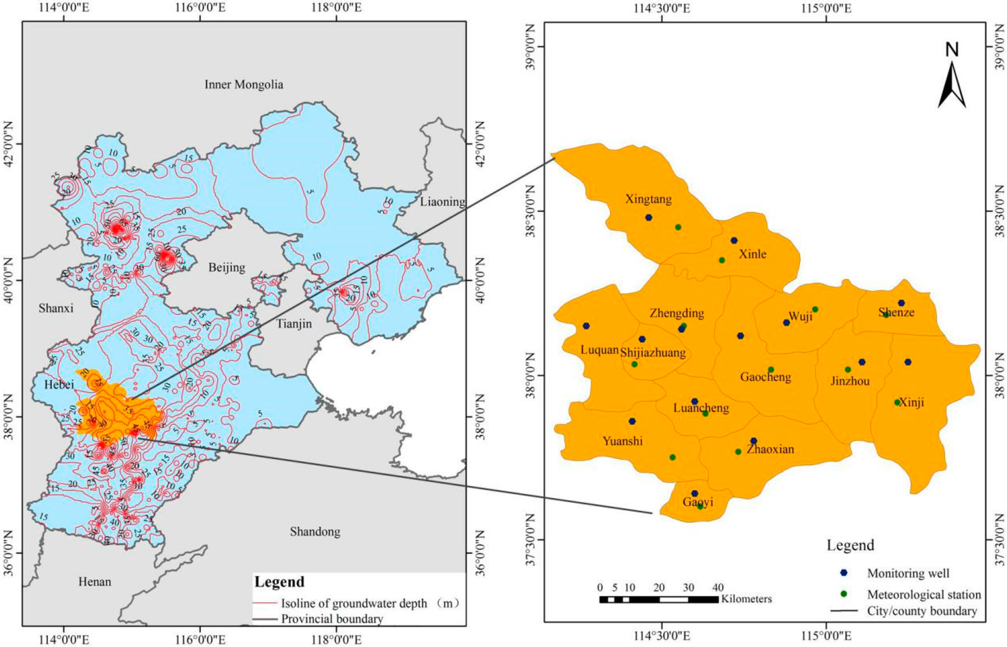
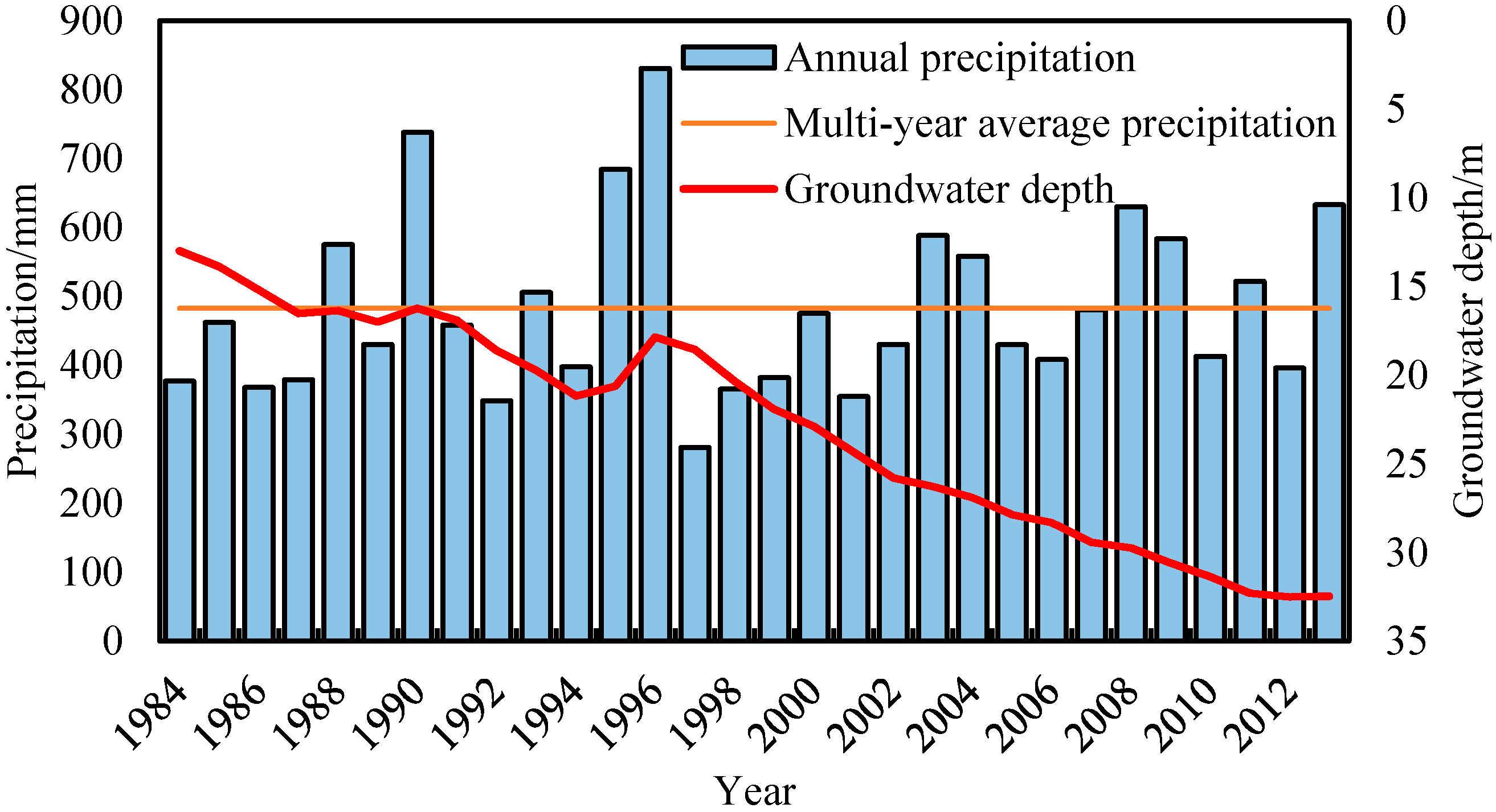
2.1. Study Area

Shijiazhuang plain (from lat 37°33′N to lat 38°42′N and from long 113°18′E to long 114°41′E) is located in central and eastern Hebei province and belongs to the Bohai Sea Economic Zone. The total area of Shijiazhuang plain is 8157 km². The average annual precipitation is about 490 mm, and the distribution is quite uneven in space and time. Over 70% of the precipitation occurs in the summer months from June to August. The average air temperature ranges from −0.8 °C in the winter seasons to 25.9 °C in the summer seasons. The plain comprises Shijiazhuang city and 13 counties, including Xingtang, Luquan, Yuanshi, Gaoyi, Xinle, Zhengding, Luancheng, Zhaoxian, Wuji, Gaocheng, Jinzhou, Xinji and Shenze. As a semi-arid region, water resources are critical to economic development and groundwater is the main source of water supply. The location of the study area and the monitoring wells and meteorological stations located in this area are shown in Figure 1. Two aquifers (the Holocene (Q4) and Upper Pleistocene (Q3)) in Shijiazhuang plain are composed of quaternary unconsolidated sediments, including sandy loam, sand and gravel-cobble. The west of Xingtang, Luquan and Yuanshi belongs to Q4, and other parts of the study area belong to Q3. The burial depth of the floor is 7–20 m for Q4 and 40–100 m for Q3. The specific field is 20–30 m³/(h·m) for Q4 and about 35 m³/(h·m) for Q3. Both of the aquifers contain a groundwater mineralization level lower than 0.5 g/L. All the 14 wells are used to monitor the shallow groundwater.

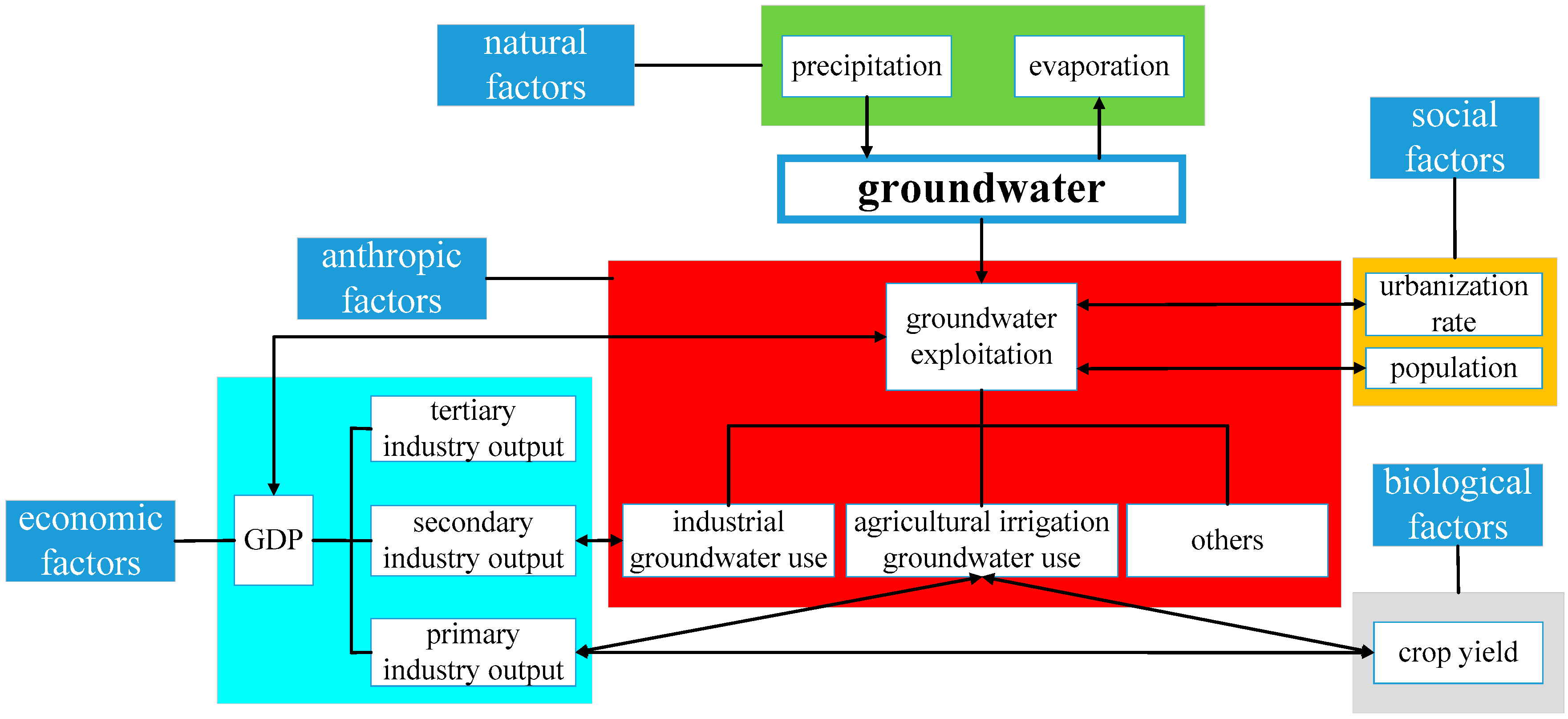
2.2. Input Indices and Data Source

Natural, anthropic, biological, economic and social factors which are closely related to the decline of the groundwater level are chosen as the key inputs of the data-driven models. These are 12 indices, including precipitation, evaporation, groundwater exploitation, industrial groundwater use, agricultural irrigation groundwater use, crop yield, population, urbanization rate, primary industry output, secondary industry output, tertiary industry output and gross domestic product (GDP). Precipitation and evaporation are the main natural factors which influence the groundwater recharge and loss. Groundwater exploitation is the groundwater fetching and use quantity, and it is the main anthropic factor which is the major reason for groundwater descending in the study area in recent decades [19], while industrial and agricultural irrigation groundwater uses are two major causes of groundwater exploitation. Crop yield is the main biological factor which reflects the crop water consumption, especially the groundwater consumption in the study area [20]. GDP is a comprehensive index indicating the regional economic strength and the pressure on groundwater use, while primary industry output, secondary industry output and tertiary industry output can reflect different aspects of economic development. Primary industry includes agriculture, forestry, animal husbandry and fishery. Secondary industry includes mining, manufacturing and construction. Tertiary industry refers to all other economic activities not included in the primary or secondary industry. Population and urbanization rate are two important factors for social development. The growth of population and the increase of urbanization rate can also raise the use of water, especially groundwater in this region.

Table 1. Serial number of the 12 input indices.

Number	Indices	Number	Indices
1	Precipitation (mm)	7	GDP (million USD)
2	Evaporation (mm)	8	Primary industry output (million USD)
3	Groundwater exploitation (million m3)	9	Secondary industry output (million USD)
4	Industrial groundwater use (million m3)	10	Tertiary industry output (million USD)
5	Irrigation groundwater use (million m3)	11	Population (million)
6	Crop yield (million ton)	12	Urbanization rate (%)

shows the serial number of the 12 indices and their mutual relations are illustrated by Figure 2.

Groundwater depth is the only index which is used to show the change of groundwater resources in this study. The higher the groundwater depth, the more scarce the groundwater resources. As located in Figure 1, 14 monitoring wells covering the whole study area are chosen to provide observational data on the annual groundwater depth from 1984 to 2013. The continuous decrease of groundwater depth can be easily observed over the 30-year period (Figure 3), and the seasonal variation of groundwater depth is obvious. The lowest groundwater level appears in summer, while the highest groundwater level can be found in winter. The groundwater depth is highly related to groundwater exploitation in different seasons for one year. In order to evaluate the groundwater of the whole study area, the average groundwater depth of 14 monitoring wells in each year is used by the models. Observed precipitation and evaporation at 13 meteorological stations are also obtained for the same period from the National Meteorological Information Center of China Meteorological Administration (available at http://www.nmic.gov.cn/). The average precipitation and evaporation from the 13 meteorological stations in each year are used as the model inputs. Thirty-year data of the other 10 input indices, including annual groundwater exploitation, industrial groundwater use, agricultural irrigation groundwater use, crop yield, population, urbanization rate, primary industry output, secondary industry output, tertiary industry output and GDP for the whole study area are also obtained for the period from 1984 to 2013. For each of the 10 input indices, annual value is the sum of the corresponding values of Shijiazhuang city and 13 counties. All the data of the 10 input indices come from the Shijiazhuang Statistical Yearbook [21].

2.3. Methodology

2.3.1. Gamma Test

The GT estimates the mean square error (MSE) that can be achieved when modelling the unseen data using any continuous nonlinear model. A formal proof of GT is given by Evans and Jones [14]. The basic idea is quite distinct from the earlier attempts with nonlinear analysis. Suppose we have a set of data observations in the form:

$$\left\{(x_{\mathrm{i}},{\mathrm{y}}_{\mathrm{i}}),1\le \mathrm{i}\le \mathrm{M}\right\}$$

(1)

where x_i ∈ R^M are input vectors confined to some closed bounded set C ∈ R^M and, y_i ∈ R are corresponding outputs. The system of GT can be expressed as the following form:

$$\mathrm{y}=\mathrm{f}(x_1\cdots x_{\mathrm{m}})+\mathrm{r}$$

(2)

where f is a smooth function and r is a random variable representing noise. Generally, the mean of the distribution of r is assumed as 0 and the variance of the noise Var(r) is bounded. The Gamma statistic Γ is the main parameter, which can estimate the model’s output variance.

For each vector x_i (1 ≤ i ≤ M), the N[i,k] are the kth (1 ≤ k ≤ p) nearest neighbors x_N[i,k] (1 ≤ k ≤ p). The distance statistic of input data can be calculated:

$${\mathsf{\delta }}_{\mathrm{M}}(\mathrm{k})=\frac{1}{\mathrm{M}}{\displaystyle \sum _{\mathrm{i}=1}^{\mathrm{M}}{\left|x_{\mathrm{N}(\mathrm{i},\mathrm{k})}-x_{\mathrm{i}}\right|}^2}(1\le k\le p)$$

(3)

where |…| denotes Euclidean distance, and the corresponding Gamma function of the output values:

$${\mathsf{\gamma }}_{\mathrm{M}}(\mathrm{k})=\frac{1}{2\mathrm{M}}{\displaystyle \sum _{\mathrm{i}=1}^{\mathrm{M}}{\left|{\mathrm{y}}_{\mathrm{N}(\mathrm{i},\mathrm{k})}-{\mathrm{y}}_{\mathrm{i}}\right|}^2}(1\le k\le p)$$

(4)

where y is the corresponding y-value for the kth nearest neighbor of x_i in Equation (3). In order to compute Γ, the p points (${\mathsf{\delta }}_{\mathrm{M}}(\mathrm{k})$, ${\mathsf{\gamma }}_{\mathrm{M}}(\mathrm{k})$) are calculated by univariate linear regression equation with least-squares:

$$\mathsf{\gamma }=\mathrm{A}\mathsf{\delta }+\mathsf{\Gamma }$$

(5)

The value of Γ is the intercept of the Equation (5). Usually, the data, which are tested by GT, are normalized to a range of 0–1. Particularly, when δ equals 0, Γ value can be computed by γ:

$${\mathsf{\gamma }}_{\mathrm{M}}(\mathrm{k})\to \text{Var}\left(r\right)\text{ in probability as }{\mathsf{\delta }}_{\mathrm{M}}(\mathrm{k})\to 0$$

(6)

A more detailed description of calculation principles can be found in Evans and Jones [14].

The V_ratio is another term, which can return a scale invariant noise estimate:

$${\mathrm{V}}_{\text{ratio}}=\frac{\mathsf{\Gamma }}{{\mathsf{\sigma }}^2(\mathrm{y})}$$

(7)

where σ²(y) is the variance of output y. According to the definition of V_ratio, the value of V_ratio close to 0 indicates a high degree of predictability of the given output y. In addition, the estimation of noise variance on the given output can be more credible if the standard error (SE) value is close to 0, and the complexity of the smooth function can be measured by the value of gradient.

2.3.2. Power Function Model (PFM)

The PFM is a kind of non-linear regression model, which is often used for prediction by establishing the relationship between the forecast factors and the forecast objects. The general equation is as follows:

$$\mathrm{y}={\mathrm{p}}_0{\mathrm{x}}_1^{{\mathrm{P}}_1}{\mathrm{x}}_2^{{\mathrm{P}}_2}\cdots {\mathrm{x}}_{\mathrm{M}}^{{\mathrm{P}}_{\mathrm{N}}}$$

(8)

where y is the forecast object, p_k (k = 0,…,N) are the parameters generally estimated by least squares and x_k (k = 1,…,M) are the explanatory variables (forecast factors).

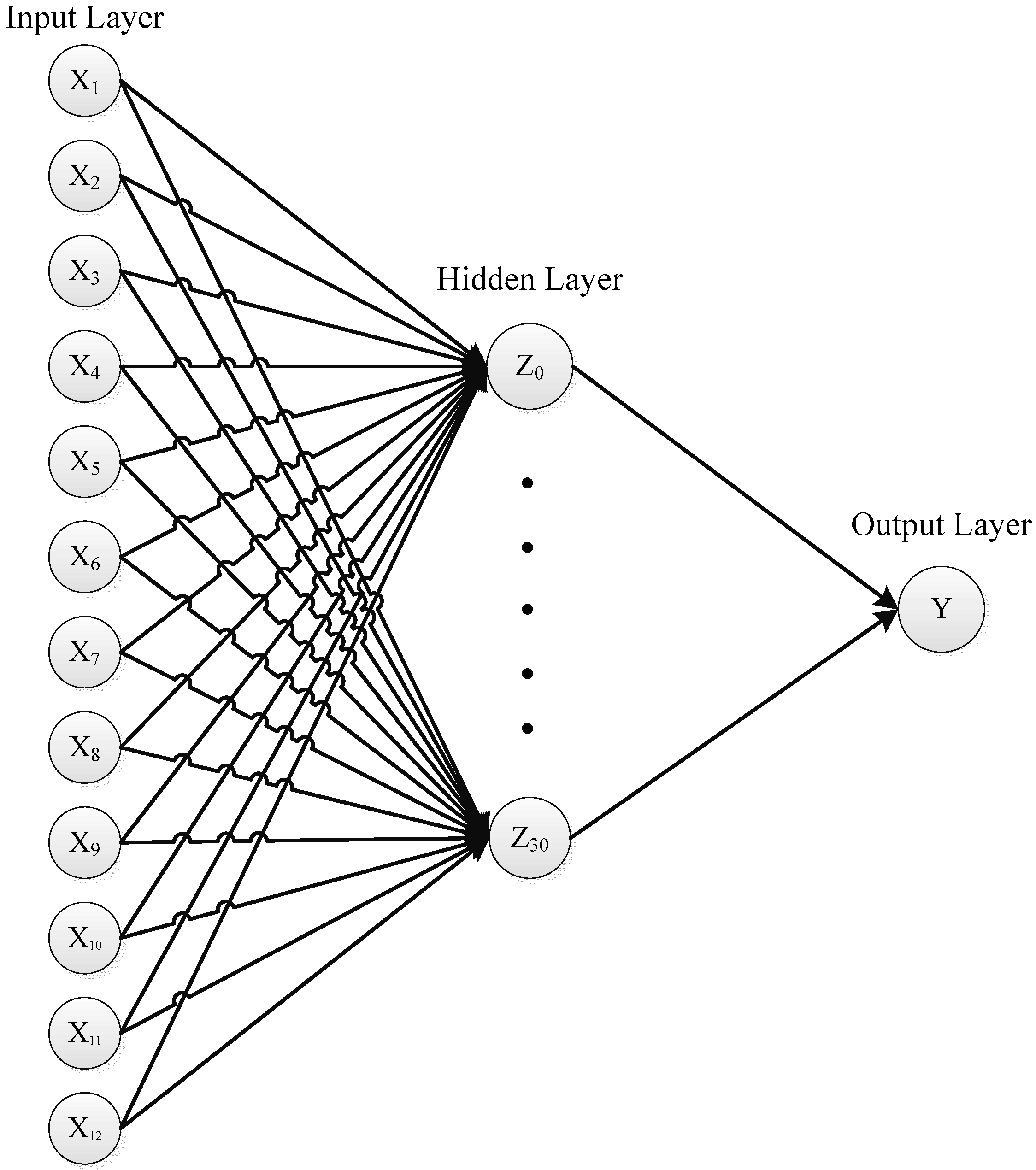
2.3.3. Back-Propagation Artificial Neural Network (BPANN)

The ANN is a nonlinear arithmetic system with densely interconnected processing elements or neurons. Three kinds of layers are contained in the mathematical structure, including input, hidden, and output layers. These layer has their nodes and activation functions. The back-propagation algorithm can effectively train the network and shorten the learning time, and it needs little information about the complex mechanism and process which should be explicitly described in mathematical form. If the neuron is the jth one in the present layer, while the inputs which it receives from the other n neurons are x₁, x₂,……,x_n, respectively, in the previous layer. The connection weights between the jth neuron and the other n neurons are w_1j, w_2j, ……, w_nj, respectively. The mathematical expression is as follows:

$${\mathrm{y}}_{\mathrm{j}}=\mathrm{f}\left({\displaystyle \sum _{\mathrm{i}=1}^{\mathrm{n}}{\mathrm{w}}_{\mathrm{i}\mathrm{j}}{\mathrm{x}}_{\mathrm{i}}+{\mathrm{b}}_{\mathrm{j}}}\right)$$

(9)

where y_j is the output of the neuron, b_j is the threshold of the neuron, and f is the transfer function.

In this study, one hidden layer is used to build the ANN model, which is trained by the back-propagation algorithm. A log-sigmoid and a linear function are contained in hidden layer and output layer, respectively. This kind of configuration is the most commonly used for ANNs, which can improve extrapolation ability. The input layer, hidden layer and output layer have five nodes, 30 nodes and one node, respectively (Figure 4). A momentum term is also added in the weight updating process to avoid the results being captured in local minimum. The number of hidden layer and nodes is discussed in Section 3.5.

2.3.4. Support Vector Machines (SVMs)

The SVM model is based on Vapnik-Chervonenkis (VC) dimension and structural risk minimum principle [22]. The SVM provides a new approach to solving the nonlinear and high dimension problem with a small sample set. The basic idea of SVM is to search for the nonlinear relationship between input and output vectors through nonlinear transformation of the input vector into the high-dimensional feature space. Given a set of N samples of ${\{x_{\mathrm{k}},{\mathrm{y}}_{\mathrm{k}}\}}_{\mathrm{k}=1}^{\mathrm{N}}$ ($x_{\mathrm{k}}$ is the input vector, ${\mathrm{y}}_{\mathrm{k}}$ is the corresponding output value), and the regression function of SVM can be expressed as:

$$\mathrm{y}=\mathrm{f}\left(x\right)=w\cdot \mathsf{\phi }\left(x\right)+\mathrm{b}$$

(10)

where w is a weight vector, $\mathsf{\phi }$ is a nonlinear transfer function that implements transformation the nonlinear to linear relationship of input to output vectors, and b is a bias. Vapnik introduced the convex quadratic optimization question to ensure that extreme solution is optimal [22], and a ε-insensitively loss function is added to Equation (10):

$$\begin{gathered} \min \mathsf{\phi }(w)=\frac{1}{2}{\Vert w\Vert }^2+\mathrm{C}{\displaystyle \sum _{\mathrm{k}=1}^{\mathrm{N}}\left({\mathsf{\xi }}_{\mathrm{k}}+{\mathsf{\xi }}_{\mathrm{k}}^{*}\right)} \\ \text{subject to}\left\{\begin{array}{c}{\mathrm{y}}_{\mathrm{k}}-w^{\mathrm{T}}\mathsf{\phi }\left(x_{\mathrm{k}}\right)-\mathrm{b}\le \mathsf{\epsilon }+{\mathsf{\xi }}_{\mathrm{k}}\\ w^{\mathrm{T}}\mathsf{\phi }\left(x_{\mathrm{k}}\right)+\mathrm{b}-{\mathrm{y}}_{\mathrm{k}}\le \mathsf{\epsilon }+{\mathsf{\xi }}_{\mathrm{k}}^{*}\\ {\mathsf{\xi }}_{\mathrm{k}},{\mathsf{\xi }}_{\mathrm{k}}^{*}\ge 0\end{array}\right\}\begin{array}{}\end{array}\mathrm{k}=1,2,\cdots ,\mathrm{N} \end{gathered}$$

(11)

where $\mathsf{\xi }$ and ${\mathsf{\xi }}^{*}$ are slack variables that penalize training errors by the loss function over the error tolerance ε, and C denotes the degree of penalization for the sample outside the error tolerance ε. The input vectors are called support vectors. The dual Lagrangian form is:

$$\mathrm{W}\left(\mathsf{\alpha },{\mathsf{\alpha }}^{*}\right)=-\frac{1}{2}{\displaystyle \sum _{\mathrm{i},\mathrm{j}=1}^{\mathrm{N}}\left({\mathsf{\alpha }}_{\mathrm{i}}-{\mathsf{\alpha }}_{\mathrm{i}}^{*}\right)({\mathsf{\alpha }}_{\mathrm{j}}-{\mathsf{\alpha }}_{\mathrm{j}}^{*})\mathrm{K}\left({\mathrm{x}}_{\mathrm{i}},{\mathrm{x}}_{\mathrm{j}}\right)+{\displaystyle \sum _{\mathrm{i}=1}^{\mathrm{N}}{\mathrm{y}}_{\mathrm{i}}\left({\mathsf{\alpha }}_{\mathrm{i}}-{\mathsf{\alpha }}_{\mathrm{i}}^{*}\right)-\mathsf{\epsilon }{\displaystyle \sum _{\mathrm{i}=1}^{\mathrm{N}}\left({\mathsf{\alpha }}_{\mathrm{i}}+{\mathsf{\alpha }}_{\mathrm{i}}^{*}\right)}}}$$

(12)

with the constraints,

$$\{\begin{array}{c}{\displaystyle \sum _{\mathrm{i}=1}^{\mathrm{N}}\left({\mathsf{\alpha }}_{\mathrm{i}}-{\mathsf{\alpha }}_{\mathrm{i}}^{*}\right)=0}\\ 0\le {\mathsf{\alpha }}_{\mathrm{i}},{\mathsf{\alpha }}_{\mathrm{i}}^{*}\le \mathrm{C}\end{array}\begin{array}{}\end{array}\left(\mathrm{i}=1,2,\cdots ,\mathrm{N}\right)$$

(13)

where α and α* are Lagrange multipliers, and the optimal desired weight vector of the regression hyperplane can be expressed with the kernel function:

$$w={\displaystyle \sum _{\mathrm{i}=1}^{\mathrm{N}}\left({\mathsf{\alpha }}_{\mathrm{i}}-{\mathsf{\alpha }}_{\mathrm{i}}^{*}\right)\mathrm{K}\left(\mathrm{x},{\mathrm{x}}_{\mathrm{i}}\right)}$$

(14)

where K(x, x_i) is the kernel function. Equation (10) can be expressed as:

$$\mathrm{y}=\mathrm{f}(x)=w\cdot \mathsf{\phi }(x)+\mathrm{b}={\displaystyle \sum _{\mathrm{i}=1}^{\mathrm{N}}\left({\mathsf{\alpha }}_{\mathrm{i}}-{\mathsf{\alpha }}_{\mathrm{i}}^{*}\right)\mathrm{K}\left(\mathrm{x},{\mathrm{x}}_{\mathrm{i}}\right)+\mathrm{b}}$$

(15)

Linear kernel function (LKF), polynomial kernel function (PKF) and radial basis function (RBF) are commonly used as kernel functions. Among these three kernel functions, the number of hyper-parameters in PKF is much more than LKF and RBF, so LKF and RBF are chosen in this study [23,24]. The parameters of RBF are discussed in Section 3.5. LKF, PKF and RBF are described by the Equations (16)–(18), respectively:

$$\mathrm{K}(\mathrm{x},{\mathrm{x}}_{\mathrm{i}})=\mathrm{x}{\mathrm{x}}_{\mathrm{i}}$$

(16)

$$\mathrm{K}(\mathrm{x},{\mathrm{x}}_{\mathrm{i}})={(1+\mathrm{x}{\mathrm{x}}_{\mathrm{i}})}^{\mathrm{d}}(d=1,2,\cdots n)$$

(17)

$$\mathrm{K}(\mathrm{x},{\mathrm{x}}_{\mathrm{i}})=\exp (-\mathsf{\gamma }\Vert \mathrm{x}-{\mathrm{x}}_{\mathrm{i}}\Vert )$$

(18)

2.3.5. Implementation and Assessment of Three Models

In this study, we define y as the groundwater depth which is an index of the groundwater dynamic variations and the forecast object, and x_k as the input factors which may influence the groundwater in the models of PFM, BPANN and SVM. PFM is constructed by the Statistical Product and Service Solutions (SPSS) software in version 19.0. BPANN and SVM are both implemented by MATLAB toolbox.

Twenty groups of data from 1984 to 2003 are used to build and train the models, while 10 groups of data from 2004 to 2013 are used for testing. All the data are normalized to a range of 0–1 to avoid disturbance of dimensions. The root mean squared error (RMSE) and Nash-Sutcliffe efficiency represented by E are used to assess the accuracy of the three built models based on the observed values and the simulated values:

$$\mathrm{R}\mathrm{M}\mathrm{S}\mathrm{E}=\sqrt{\frac{1}{\mathrm{N}}{\displaystyle \sum _{\mathrm{i}=1}^{\mathrm{N}}{\left({\widehat{\mathrm{y}}}_{\mathrm{i}}-{\mathrm{y}}_{\mathrm{i}}\right)}^2}}$$

(19)

$$\mathrm{E}=1-{\displaystyle \sum _{\mathrm{i}=1}^{\mathrm{N}}{({\stackrel{⌢}{\mathrm{y}}}_{\mathrm{i}}-{\mathrm{y}}_{\mathrm{i}})}^2}/{\displaystyle \sum _{\mathrm{i}=1}^{\mathrm{N}}{({\mathrm{y}}_{\mathrm{i}}-{\overline{\mathrm{y}}}_{\mathrm{i}})}^2}$$

(20)

where y_i and ${\widehat{\mathrm{y}}}_{\mathrm{i}}$ are the observed and simulated values of groundwater depth, respectively, ${\overline{\mathrm{y}}}_{\mathrm{i}}$ is the mean observed value, i = 1,2,…,N, and N is the number of data groups. The perfect scores of RMSE and E are 0 and 1, respectively.

3. Results

3.1. Correlation Test for 12 Inputs

Pearson correlation coefficients (ρ) are used to analyze the correlations among the 12 inputs. The value of 1 means a perfect positive correlation while the value of −1 means a perfect negative correlation. The correlation coefficients of the 12 inputs are shown in

Table 2. Correlation test for 12 inputs.

Inputs Number	Correlation Coefficient (ρ)
	1	2	3	4	5	6	7	8	9	10	11	12
1	1
2	−0.199	1
3	−0.360	0.376	1
4	−0.225	−0.176	−0.115	1
5	−0.355	0.346	0.352	0.190	1
6	0.122	0.357	0.406	−0.234	0.175	1
7	0.131	0.211	0.168	−0.410	−0.175	0.309	1
8	0.139	0.315	0.250	−0.392	−0.105	0.324	0.432	1
9	0.135	0.217	0.167	−0.387	−0.178	0.309	0.799 *	0.282	1
10	0.131	0.189	0.150	−0.288	−0.189	0.388	0.399	0.376	0.398	1
11	0.150	0.313	0.323	−0.381	−0.049	0.385	0.430	0.371	0.328	0.720 *	1
12	0.154	0.146	0.238	−0.324	−0.160	0.217	0.455	0.347	0.354	0.351	0.440	1

Note: * means significant at 0.05 level.

. Most correlation coefficients are lower than 0.5 and most inputs show weak correlations. However, the correlation coefficient between GDP and secondary industry output reach 0.799, which indicates that secondary industry output is the main means to improve the economy in Shijiazhuang plain. Tertiary industry output also has a high correlation with population, which means that tertiary industry is greatly influenced by population in the study area. Though the two pairs of inputs have relatively high correlation coefficients, overall, the correlations among the 12 inputs have little effect on the feature selection results.

3.2. Relative Importance of the Model Inputs

The GT can provide the least model error compared to any smooth model by only giving the input and output data. In the study, the Gamma value Γ is used as the main criterion for distinguishing the importance of model inputs and the other three factors produced by GT (i.e., Gradient, Standard error of Γ and V_ratio) are used as a reference. This is because there are still some technical problems of GT that cannot be explained in detail, such as the utilization of the three factors (Gradient, Standard error of Γ and V_ratio). Basically, the least |Γ| represents the best model input combination. The gradient can indicate the model complexity. The lower the gradient, the more simple the model should be fitted. The SE of Γ shows the reliability of the Gamma value. The higher it is, the more unreliable the Gamma value is. V_ratio illustrates the predictability of outputs using the effective inputs [15]. A mathematical model (e.g., PFM, BPANN and SVM in this study) may be built in high quality, if the three factors (gradient, SE of Γ and V_ratio) show low values by setting the best input data [17].

Table 3. GT results for schemes with different combinations of model input indices.

Scheme ID	Combination of Indices	Masked Index	Gamma (Γ)	Gradient	Standard Error	Vratio
1	1,2,3,4,5,6,7,8,9,10,11,12	None	−0.00922	0.02841	0.01161	−0.03687
2	2,3,4,5,6,7,8,9,10,11,12	1	−0.00212	0.02529	0.00420	−0.00848
3	1,3,4,5,6,7,8,9,10,11,12	2	−0.00170	0.02776	0.00612	−0.00679
4	1,2,4,5,6,7,8,9,10,11,12	3	−0.00836	0.03004	0.00767	−0.03343
5	1,2,3,5,6,7,8,9,10,11,12	4	−0.01020	0.03265	0.00566	−0.04082
6	1,2,3,4,6,7,8,9,10,11,12	5	−0.00732	0.03007	0.00711	−0.02927
7	1,2,3,4,5,7,8,9,10,11,12	6	−0.00559	0.02845	0.00606	−0.02235
8	1,2,3,4,5,6,8,9,10,11,12	7	−0.00714	0.02955	0.00510	−0.02857
9	1,2,3,4,5,6,7,9,10,11,12	8	−0.00580	0.02850	0.00613	−0.02320
10	1,2,3,4,5,6,7,8,10,11,12	9	−0.00745	0.02944	0.00993	−0.02981
11	1,2,3,4,5,6,7,8,9,11,12	10	−0.00316	0.02759	0.00739	−0.01264
12	1,2,3,4,5,6,7,8,9,10,12	11	−0.00351	0.02842	0.00810	−0.01405
13	1,2,3,4,5,6,7,8,9,10,11	12	−0.01372	0.03514	0.00919	−0.05487

shows the GT results for schemes with different combinations of model input indices listed in Table 1. Scheme 1 involves all 12 input indices and the other schemes have 11 indices with the rest masked. It is interesting to find that only Scheme 5 (without index 4, i.e., industrial groundwater use) and Scheme 13 (without index 12, i.e., urbanization rate) have larger |Γ| values than Scheme 1. The other schemes all have smaller |Γ| values which indicate they will perform better than Scheme 1 in constructing a reliable model. It can be seen from Table 3 that the best combination of indices is in Scheme 3 which has the least |Γ| (0.00170), and the worst combination of indices is in Scheme 13 which has the highest |Γ| (0.01372). Then, we can rank the schemes from best to worst, which is 3 > 2 > 11 > 12 > 7 > 9 > 8 > 6 > 10 > 4 > 1 > 5 > 13, and the missing index in each of the schemes can form a ranking of the importance of the model input indices, which is 2 < 1 < 10 < 11 < 6 < 8 < 7 < 5 < 9 < 3 < 4 < 12. This indicates that natural factors (precipitation and evaporation) have less effect on the groundwater level, while anthropic factors, biological factors, economic factors and social factors have greater influence. Urbanization rate and industrial groundwater use are the two most important model input indices which imply that the process of modernization and industrial development in Shijiazhuang plain is the main cause of groundwater recession.

3.3. Model Input Selection Based on Gamma Test

In order to find the best combination of model inputs, search methods of backward and forward selections are coupled with the GT [25]. The backward procedure starts with all indices and each index is gradually removed in turn, while the forward procedure starts with the minimum index number and carries on by adding one index at a time successively. The index which works the best with the indices from the last round (i.e., resulting in the least |Γ| value) is added in forward selection and the one with the absence of which leads to the best results is removed in backward selection. The procedure is iterated until one index is left for backward selection or until all indices are included for forward selection.

Table 4. Backward selection results with the assistance of GT.

Scheme ID	Combination of Indices	Index Removed	Gamma (Γ)	Gradient	Standard Error	Vratio
1	1,2,3,4,5,6,7,8,9,10,11,12	None	−0.00922	0.02841	0.01161	−0.03687
3	1,3,4,5,6,7,8,9,10,11,12	2	−0.00170	0.02776	0.00612	−0.00679
14	1,3,4,5,6,7,8,9,10,12	11	0.00103	0.02878	0.00555	0.00413
15	3,4,5,6,7,8,9,10,12	1	0.00031	0.03579	0.00625	0.00124
16	3,4,5,6,7,9,10,12	8	−0.00014	0.03999	0.00916	−0.00054
17	3,4,5,6,9,10,12	7	0.00021	0.04415	0.00776	0.00085
18	3,4,5,6,9,12	10	0.00091	0.05043	0.00736	0.00366
19	3,4,6,9,12	5	−0.00006	0.06856	0.00886	−0.00023
20	3,4,6,12	9	0.00160	0.08593	0.00660	0.00640
21	3,4,12	6	0.01719	0.08515	0.01186	0.06877
22	4,12	3	0.02153	0.15409	0.01040	0.08612
23	12	4	0.00546	0.71495	0.00361	0.02185

and

Table 5. Forward selection results with the assistance of GT.

Scheme ID	Combination of Indices	Index added	Gamma (Γ)	Gradient	Standard Error	Vratio
23	12	None	0.00546	0.71495	0.00361	0.02185
24	10,12	10	0.00285	0.19576	0.00491	0.01142
25	7,10,12	7	0.00149	0.13163	0.00483	0.00597
26	6,7,10,12	6	0.00645	0.08496	0.00294	0.02579
27	3,6,7,10,12	3	−0.00069	0.07638	0.00797	−0.00277
28	3,4,6,7,10,12	4	0.00199	0.05354	0.00541	0.00796
29	3,4,5,6,7,10,12	5	0.00134	0.04241	0.00717	0.00539
16	3,4,5,6,7,9,10,12	9	−0.00014	0.03999	0.00916	−0.00054
15	3,4,5,6,7,8,9,10,12	8	0.00031	0.03579	0.00625	0.00124
14	1,3,4,5,6,7,8,9,10,12	1	0.00103	0.02878	0.00555	0.00414
3	1,3,4,5,6,7,8,9,10,11,12	11	−0.00170	0.02776	0.00612	−0.00679
1	1,2,3,4,5,6,7,8,9,10,11,12	2	−0.00922	0.02841	0.01161	−0.03687

show the model input selection results by using the search methods of backward and forward selections coupled with the GT, respectively. It can be found from the two tables that Scheme 19 has relatively fewer indices and the smallest values of |Γ| (0.00006). Theoretically, because of the least |Γ| and relatively fewer indices, Scheme 19 is the best model input combination. In this study, Scheme 19 is used to construct the three models. However, GT is still a method which requires more experiments to be completed. In order to make our conclusions more reliable, all the schemes in Table 4 and Table 5 are calculated as part of the sensitivity analysis of the input choice in Section 3.6.

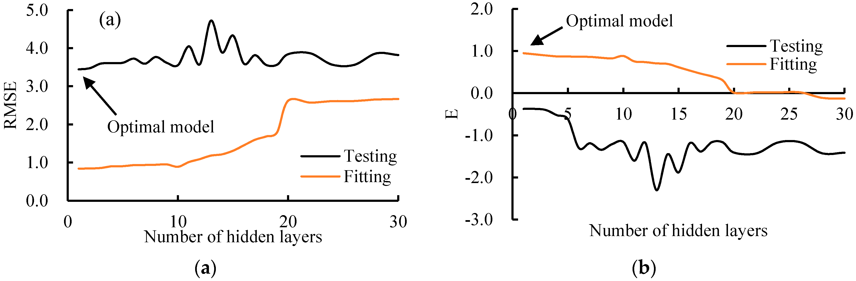
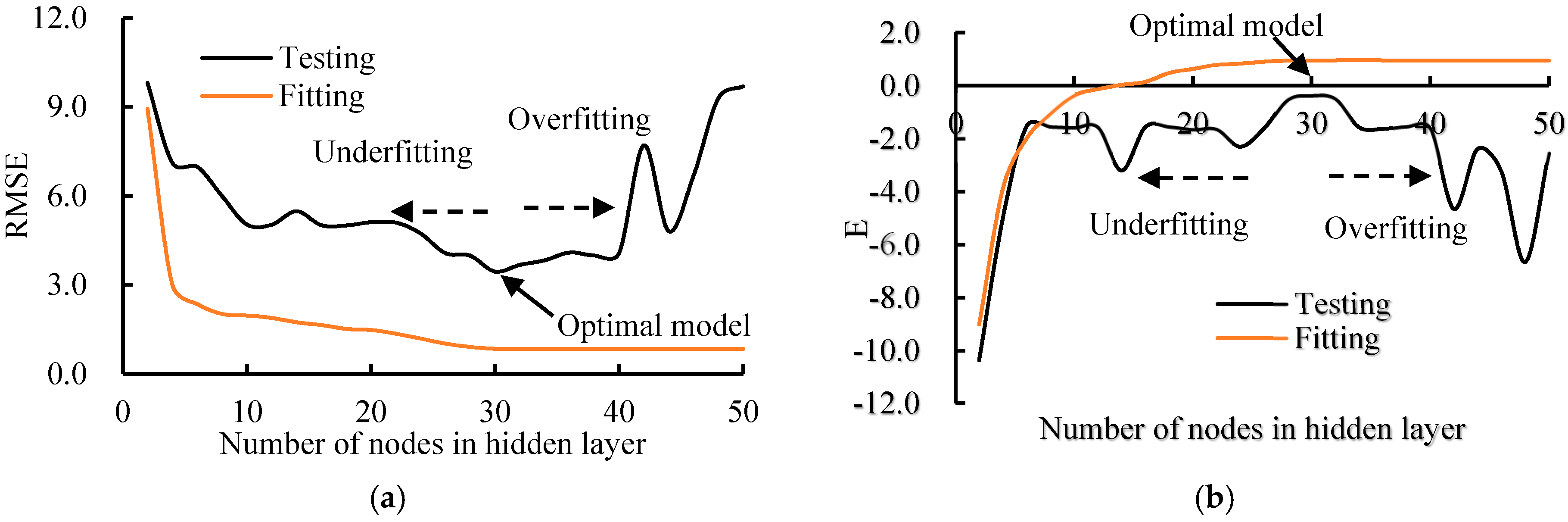
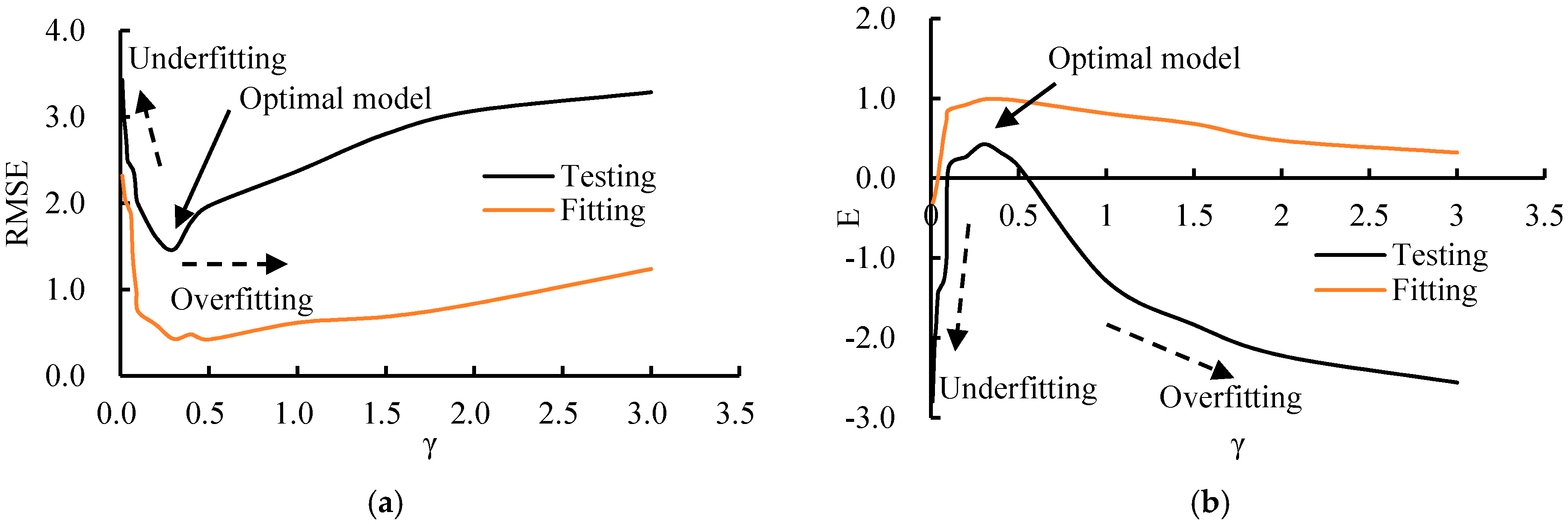
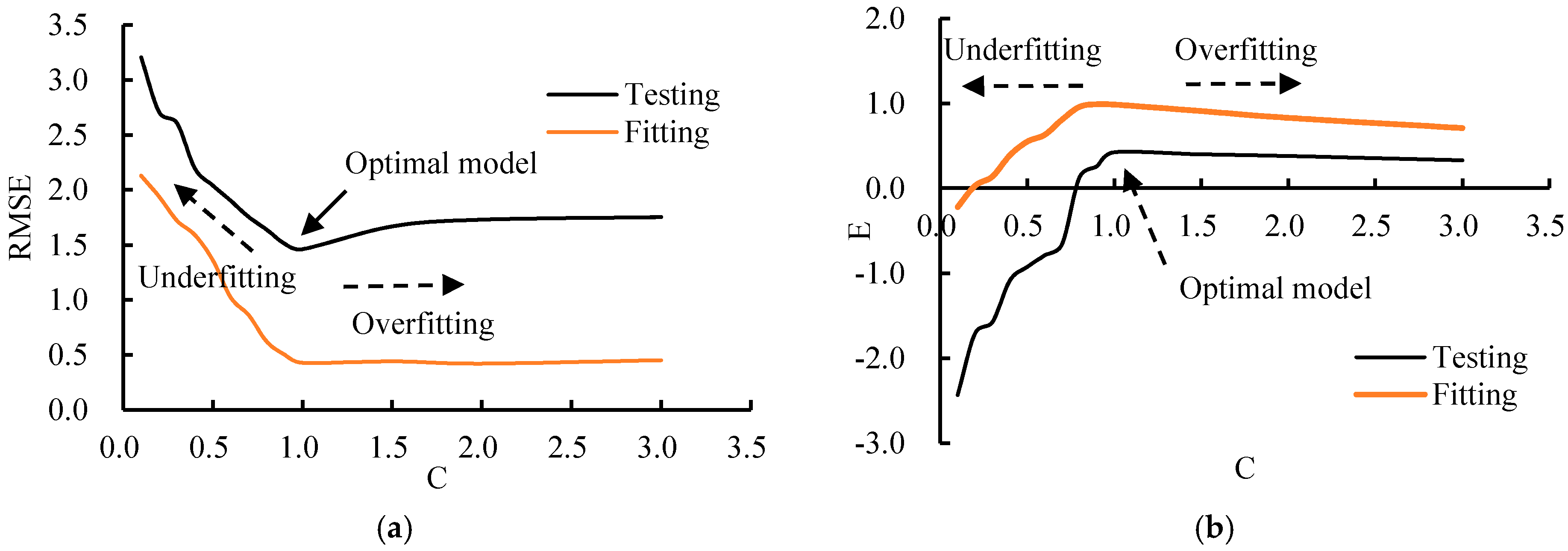
3.4. Influence of the Parameters in BPANN and SVM (RBF)

Possible data overfitting is a disadvantage of BPANN and SVM (RBF). In order to avoid this problem and make the models more accurate, we choose the hidden layers and nodes for BPANN and two parameters (C and γ) for SVM (RBF) carefully by means of the try-and-error method. The parameter C which is a positive trade-off parameter determines the degree of empirical error and the parameter γ which is the main parameter in kernel function of RBF. Numerous trials were conducted.

Taking Scheme 19 as an example, the optimum numbers of hidden layers and nodes per layer are 1 and 30 for BPANN, respectively, while the optimal values of C and γ in this study are chosen to be 1.0 and 0.3 for SVM (RBF), respectively. All these optimal parameters are chosen based on the values of RMSE and E. With the change in number of hidden layers and nodes, different values of RMSE and E can be seen in Figure 5 and Figure 6. The influences of the C and γ on the testing results are shown in Figure 7 and Figure 8.

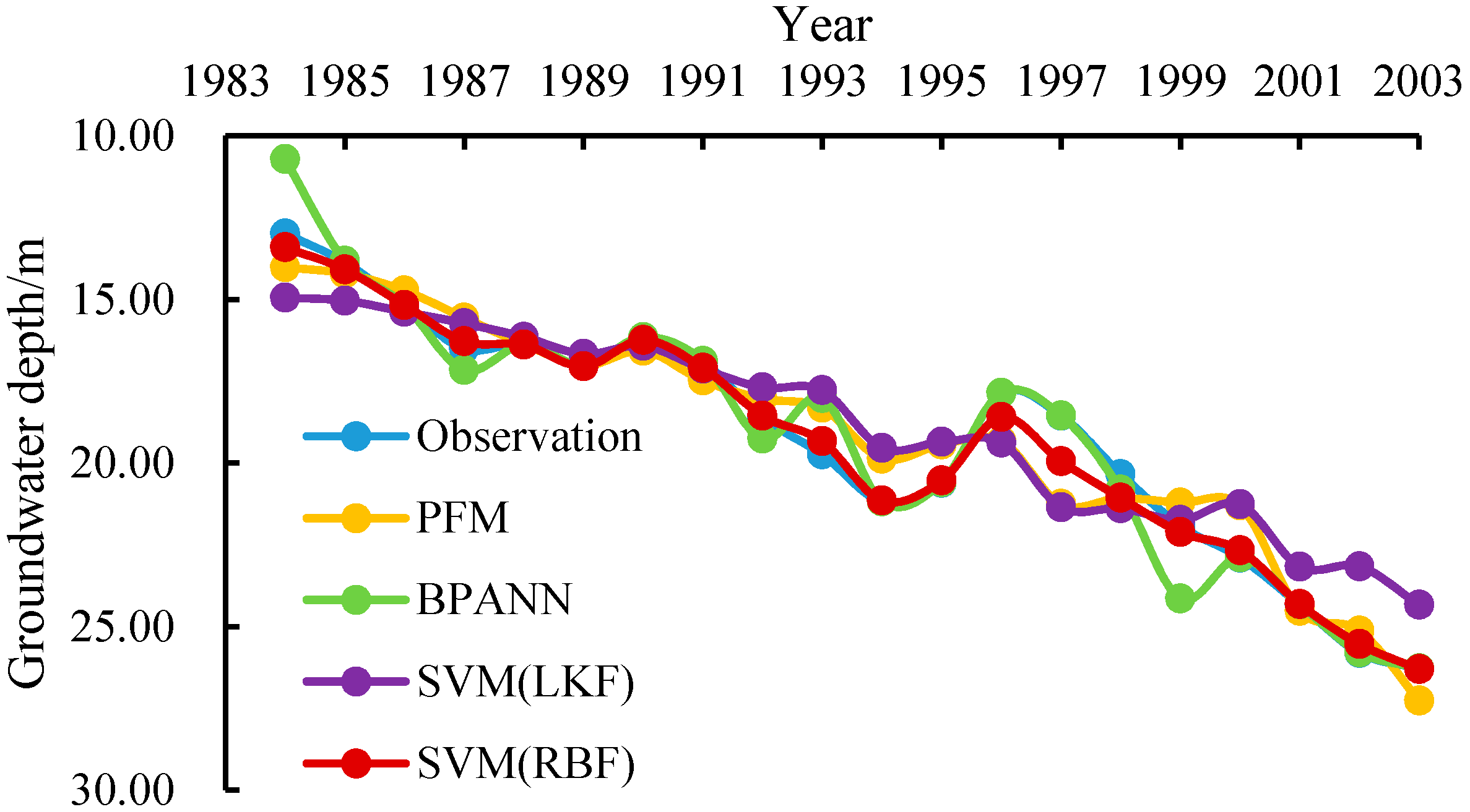
3.5. Fitting Results and Model Errors

For Scheme 19, the equation of PFM can be expressed as follows calibrated on the 20 groups of data from 1984 to 2003, respectively:

$$\widehat{\mathrm{y}}=0.0015{\mathrm{x}}_3^{0.2961}{\mathrm{x}}_4^{0.2428}{\mathrm{x}}_6^{0.1144}{\mathrm{x}}_9^{0.0009}{\mathrm{x}}_{12}^{0.4832}$$

(21)

where x₃ is groundwater exploitation, x₄ is industrial groundwater use, x₆ is crop yield, x₉ is secondary industry output and x₁₂ is urbanization rate, $\widehat{\mathrm{y}}$ is the fitting results for groundwater depth.

The other two models of BPANN and SVM are also trained based on the dataset from 1984 to 2003. The procedure is carried out several times for both models and the optimal results are adopted. The RMSE and E of the three models for fitting results are shown in

Table 6. Fitting results and errors of PFM, BPANN and SVM models for Scheme 19.

Scheme ID	PFM		BPANN		SVM (LKF)		SVM (RBF)
	RMSE	E	RMSE	E	RMSE	E	RMSE	E
19	1.0638	0.9157	0.8411	0.9473	1.4345	0.8467	0.4265	0.9864

.

The RMSEs of PFM and SVM (LKF) are both higher than 1.0, and the value of SVM (LKF) is close to 1.5. The RMSE is lower than 0.5 for the SVM (RBF) model, while the value of BPANN model is higher than 0.5 and lower than PFM and SVM (LKF). So, the fitting values of SVM (RBF) are closer to observed values. The highest values of E are near 1.0 for SVM (RBF), and the lowest values of E are lower than 0.85 for SVM (LKF). It indicates that SVM (RBF) has the highest reliability in the four models. Based on the values of RMSE and E, it can be easily observed that the SVM (RBF) model has the best generalization ability in the sample learning process, while the SVM (LKF) model performs the worst. Good fitting results do not mean good prediction ability for the data-driven models. The performance of the models needs to be tested with further datasets. The observed and fitted values (Scheme 19) of groundwater depth are shown in Figure 9.

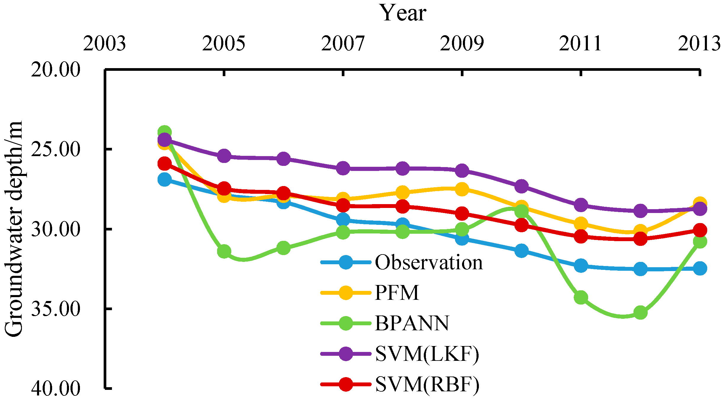
3.6. Testing Results and Model Errors

The three types of data-driven models are tested based on the 10 groups of data from 2004 to 2013 for three schemes. The RMSE and E of the three models for testing results are shown in

Table 7. Testing results and errors of PFM, BPANN and SVM models for Scheme 19.

Scheme ID	PFM		BPANN		SVM (LKF)		SVM (RBF)
	RMSE	E	RMSE	E	RMSE	E	RMSE	E
19	2.3916	−0.5409	2.2597	−0.3755	3.4417	−2.1910	1.4612	0.4248

. For Scheme 19, only the RMSE of SVM (RBF) is lower than 2.0, and the RMSE of SVM (LKF) is higher than 3.0. The BPANN model has lower RMSE than the PFM model. The value of E is higher than 0 for SVM (RBF), and the lowest values of E are lower than −2.0 for PFM and SVM (LKF). It can be noticed that BPANN and SVM (RBF) models perform better than PFM and SVM (LKF) as a whole with a relatively lower RMSE and better E, but stability is poor for the BPANN model. The SVM (RBF) model performs best in the testing process, and it has generalization ability in the testing process. The observed and tested values (Scheme 19) of groundwater depth are shown in Figure 10.

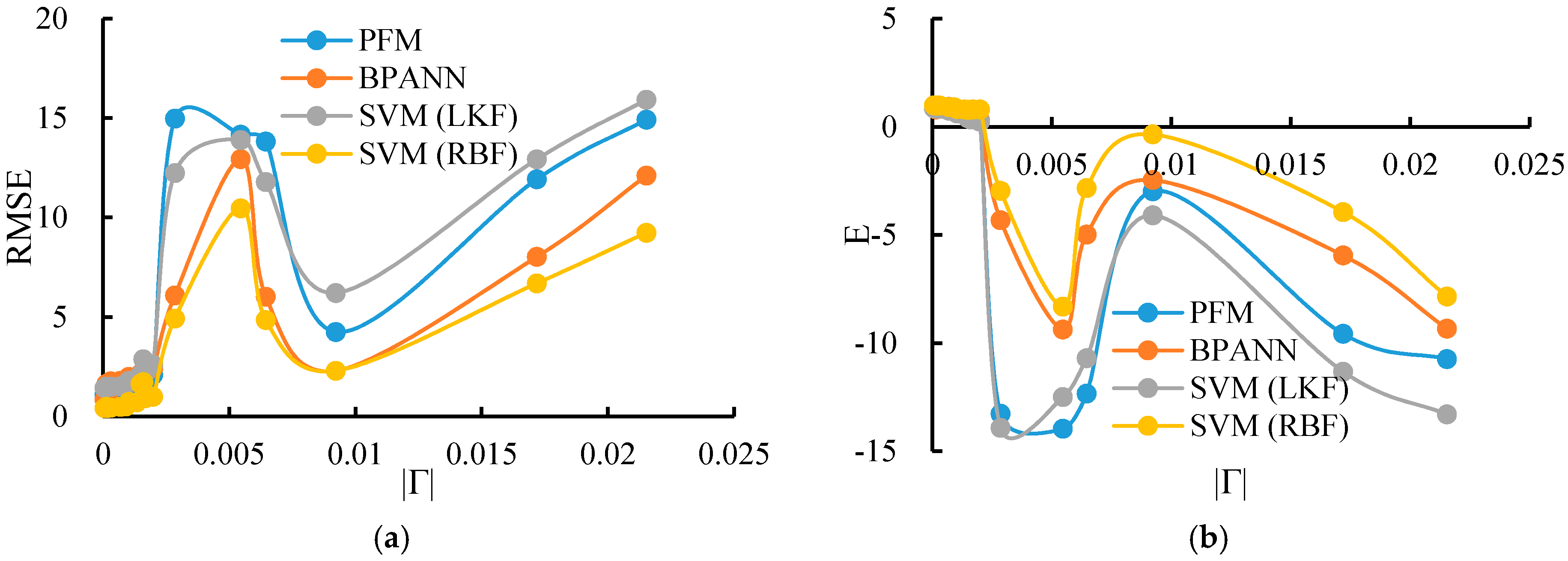
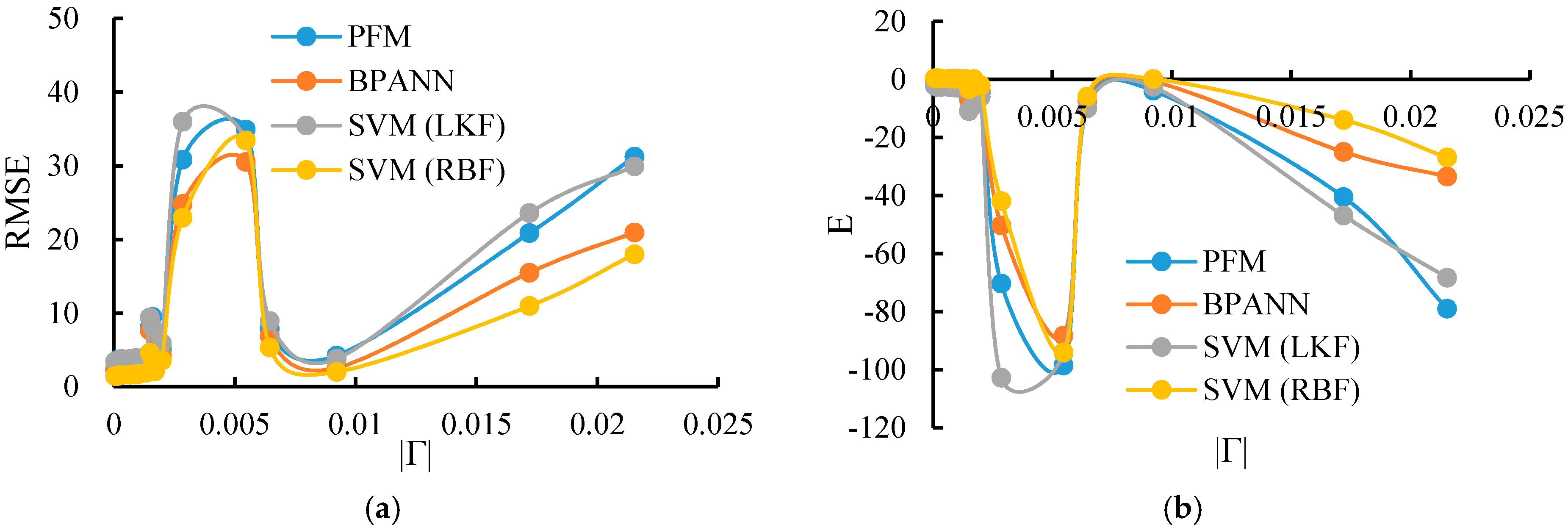
3.7. Sensitivity Analysis of the Input Choice

In order to make the input choice conclusion more reliable, the same methods are used to calculate the values of RMSE and E for other schemes in Table 4 and Table 5, and the results are compared with Scheme 19. The optimal models for BPANN and SVM (RBF) are also chosen by testing the influence of the parameters in the models. The fitting and testing results and errors of PFM, BPANN and SVM models are shown in

Table 8. Fitting results and errors of PFM, BPANN and SVM models.

Scheme ID	Gamma (Γ)	PFM		BPANN		SVM (LKF)		SVM (RBF)
		RMSE	E	RMSE	E	RMSE	E	RMSE	E
19	−0.00006	1.0638	0.9157	0.8411	0.9473	1.4345	0.8467	0.4265	0.9864
16	−0.00014	1.1770	0.8968	1.6441	0.7986	1.4995	0.8351	0.4868	0.9823
17	0.00021	1.1626	0.8993	0.9923	0.9266	1.4874	0.8325	0.4279	0.9864
15	0.00031	1.2342	0.8801	1.7692	0.9359	1.5033	0.8302	0.4427	0.9821
27	−0.00069	1.3094	0.7908	1.7903	0.9137	1.5232	0.7365	0.4915	0.9122
18	0.00091	1.2942	0.7882	1.8233	0.8244	1.6044	0.7086	0.5111	0.9035
14	0.00103	1.5336	0.6627	1.9917	0.6823	1.7908	0.6109	0.7293	0.8146
29	0.00134	1.6092	0.5634	1.9737	0.5605	1.7834	0.5701	0.7184	0.8003
25	0.00149	1.8864	0.4101	2.1431	0.4023	2.0937	0.3952	1.6436	0.7822
20	0.00160	1.6903	0.4629	2.2098	0.3857	2.8806	0.3328	1.7305	0.7909
3	−0.00170	1.6805	0.4307	2.3105	0.3632	2.2308	0.3586	0.9236	0.8013
28	0.00199	2.0937	0.2956	2.4208	0.2924	2.6011	0.2393	0.9937	0.8028
24	0.00285	14.9721	−13.2698	6.0912	−4.3223	12.2426	−13.9142	4.9251	−2.9634
23	0.00546	14.1693	−13.9601	12.9411	−9.3762	13.9031	−12.4881	10.4623	−8.3092
26	0.00645	13.8233	−12.3302	6.0265	−4.9808	11.7868	−10.6984	4.8521	−2.8341
1	−0.00922	4.2475	−2.9804	2.2928	−2.4636	6.2099	−4.0928	2.2947	−0.3525
21	0.01719	11.9236	−9.5725	8.0231	−5.9467	12.9325	−11.3207	6.6943	−3.9408
22	0.02153	14.9261	−10.7363	12.1099	−9.3307	15.9222	−13.2903	9.2362	−7.8460

and

Table 9. Testing results and errors of PFM, BPANN and SVM models.

Scheme ID	Gamma (Γ)	PFM		BPANN		SVM (LKF)		SVM (RBF)
		RMSE	E	RMSE	E	RMSE	E	RMSE	E
19	−0.00006	2.3916	−0.5409	2.2597	−0.3755	3.4417	−2.191	1.4612	0.4248
16	−0.00014	3.6501	−2.5891	2.5698	−0.7791	3.4791	−2.2608	1.4359	0.4446
17	0.00021	3.1715	−1.7097	2.2831	−0.4042	3.4125	−2.1371	1.5822	0.3256
15	0.00031	3.7253	−2.5912	2.4672	−0.7923	3.7982	−2.6952	1.5901	0.3083
27	−0.00069	3.7526	−2.6108	2.5094	−0.8155	3.8023	−2.7325	1.6433	0.2596
18	0.00091	3.7802	−2.7941	2.6455	−0.9406	3.9246	−2.8244	1.7024	0.2319
14	0.00103	3.8204	−2.7992	2.5123	−0.8299	3.4819	−2.4953	1.7293	0.2297
29	0.00134	3.8246	−2.8456	2.5297	−0.8482	4.1284	−3.2349	1.9039	0.2006
25	0.00149	8.0644	−10.936	7.6436	−7.0354	9.423	−10.843	4.6255	−3.4251
20	0.00160	9.5036	−9.4213	7.9928	−8.3409	8.1567	−9.6242	3.9288	−2.8603
3	−0.00170	4.8355	−3.2194	2.4093	−0.7021	3.6938	−3.0365	2.0934	0.1353
28	0.00199	5.1032	−4.9412	4.2356	−3.9236	5.9435	−6.0256	3.5647	−2.0425
24	0.00285	30.8291	−70.3527	24.821	−50.3423	35.9801	−102.8313	22.9564	−41.9327
23	0.00546	34.9115	−98.5744	30.5092	−88.3257	33.4883	−94.2952	33.4219	−94.0942
26	0.00645	7.9212	−7.2205	6.9023	−6.8211	8.9346	−9.9438	5.3196	−5.9443
1	−0.00922	4.2245	−3.9231	2.5646	−0.7924	3.7992	−2.5871	2.0293	0.1212
21	0.01719	20.8431	−40.5496	15.4925	−24.9825	23.5794	−46.9324	10.9577	−13.9548
22	0.02153	31.2469	−79.0362	20.9421	−33.4924	29.91207	−68.3629	17.9822	−26.9293

. Figure 11 and Figure 12 show the changes of RMSE and E with |Γ|. It indicates that Scheme 19 is the best model input combination with lower values of RMSE and E for the three models, and it also has relatively fewer indices. Overall, with the increase of the |Γ|, the performances of the three models become worse, so GT can be used to confirm the best combination of model inputs. It should be mentioned that Schemes 21, 22, 23, 24 and 26 with much fewer indices have much higher RMSE and lower E. So, the schemes with much fewer indices but smaller values of |Γ| should be tested carefully. Additionally, it also can be seen that the SVM (RBF) performs best in most schemes.

4. Discussion and Conclusions

Considering limited data and complicated geological conditions in the plain of Shijiazhuang, physical models are not a good choice, and three types of data-driven models are used in this study to predict the groundwater depth in Shijiazhuang plain. Five kinds of factors (natural, anthropic, biological, economic and social) including 12 indices which may influence the groundwater depth are considered, i.e., precipitation, evaporation, groundwater exploitation, industrial groundwater use, agricultural irrigation groundwater use, crop yield, population, urbanization rate, primary industry output, secondary industry output, tertiary industry output and GDP. An efficient tool named GT is adopted in this study to identify the relative importance of the indices and further determine the best model input combination. The results of GT indicate that natural factors (precipitation and evaporation) have less effect on the groundwater level, while anthropic factors, biological factors, economic factors and social factors are the main reasons for the groundwater level decline, especially the anthropic factors which reflect the groundwater exploitation. Evaporation is found to be the least relevant index among the 12 indices, while urbanization rate and industrial groundwater use are shown to have the most significant effect on groundwater variations. This indicates that the relationship between the evaporation and the groundwater becomes weaker with the drop in groundwater level. It also reveals that modernization and industrial development in Shijiazhuang plain are the main reasons for groundwater recession.

The RMSE and E are used to assess the accuracy of the data-driven models. The results show that BPANN and SVM (RBF) models perform better than PFM and SVM (LKF) as a whole in all three schemes, while SVM (RBF) has the best generalization ability during the fitting and testing process. The SVM (RBF) model performs the best in both model fitting and model testing. Additionally, all the schemes in Table 4 and Table 5 are used to analyze the sensitivity of the input choice. The results show that GT can be used to confirm the best combination of model inputs, but schemes with much fewer indices and smaller values of |Γ| should be tested carefully.

The groundwater level has decreased dramatically and is continuing to do so in Shijiazhuang plain. Countermeasures need to be taken to reduce groundwater usage and guarantee the sustainable utilization of groundwater, by improving the water use efficiency, promoting comprehensive water-saving measures, adjusting the industrial structure and finding alternative water sources, such as water recycling and the South-to-North Water Diversion Project. The results of this study may also provide a methodology and a reference for the prediction of groundwater resources in data-limited areas, especially for the study region and North China in general. However, monthly prediction of the groundwater depth has not been considered in this study due to limited data observations. The advantage of GT can be better exploited when dealing with larger datasets using data-driven models in groundwater prediction.

References

1. Cao, G.; Zheng, C.; Scanlon, B.R.; Liu, J.; Li, W. Use of flow modeling to assess sustainability of groundwater resources in the North China Plain. Water Resour. Res. 2013, 49, 159–175. [Google Scholar] [CrossRef]
2. Natkhin, M.; Steidl, J.; Dietrich, O.; Dannowski, R.; Lischeid, G. Differentiating between climate effects and forest growth dynamics effects on decreasing groundwater recharge in a lowland region in Northeast Germany. J. Hydrol. 2012, 448, 245–254. [Google Scholar] [CrossRef]
3. Goderniaux, P.; Brouyère, S.; Wildemeersch, S.; Therrien, R.; Dassargues, A. Uncertainty of climate change impact on groundwater reserves—Application to a chalk aquifer. J. Hydrol. 2015, 528, 108–121. [Google Scholar] [CrossRef]
4. Yuan, Z.; Shen, Y. Estimation of agricultural water consumption from meteorological and yield data: A case study of Hebei, North China. PLoS ONE 2013, 8, e58685–e58685. [Google Scholar] [CrossRef] [PubMed]
5. Davidsen, C.; Liu, S.; Mo, X.; Rosbjerg, D.; Bauer-Gottwein, P. The cost of ending groundwater overdraft on the North China Plain. Hydrol. Earth Syst. Sci. 2015, 12, 5931–5966. [Google Scholar] [CrossRef]
6. Kendy, E.; Gérard-Marchant, P.; Walter, M.T.; Zhang, Y.; Liu, C.; Tammo, S.S. A soil-water-balance approach to quantify groundwater recharge from irrigated cropland in the North China Plain. Hydrol. Process. 2003, 17, 2011–2031. [Google Scholar] [CrossRef]
7. Hu, Y.; Moiwo, J.P.; Yang, Y.; Han, S.; Yang, Y. Agricultural water-saving and sustainable groundwater management in Shijiazhuang Irrigation District, North China Plain. J. Hydrol. 2010, 393, 219–232. [Google Scholar] [CrossRef]
8. Knotters, M.; Bierkens, M.F.P. Physical basis of time series models for water table depths. Water Resour. Res. 2000, 36, 181–188. [Google Scholar] [CrossRef]
9. Asefa, T.; Kemblowski, M.; Urroz, G.; Mckee, M. Support vector machines (SVMs) for monitoring network design. Groundwater 2005, 43, 413–422. [Google Scholar] [CrossRef] [PubMed]
10. Xu, T.F.; Valocchi, A.J.; Choi, J.; Amir, E. Use of machine learning methods to reduce predictive error of groundwater models. Groundwater 2013, 52, 448–460. [Google Scholar] [CrossRef] [PubMed]
11. Yang, Z.P.; Lu, W.X.; Long, Y.Q.; Li, P. Application and comparison of two prediction models for groundwater levels: A case study in Western Jilin Province, China. J. Arid Environ. 2009, 73, 487–492. [Google Scholar] [CrossRef]
12. Shirmohammadi, B.; Vafakhah, M.; Moosavi, V.; Moghaddamnia, A. Application of several data-driven techniques for predicting groundwater level. Water Resour. Manag. 2013, 27, 419–432. [Google Scholar] [CrossRef]
13. Ping, J.; Qiang, Y.; Xi, M. A combination model of chaos, wavelet and support vector machine predicting groundwater levels and its evaluation using three comprehensive quantifying techniques. Inf. Technol. J. 2013, 12, 3158–3163. [Google Scholar] [CrossRef]
14. Evans, D.; Jones, A.J. A proof of the Gamma test. Proc. R. Soc. Lond. A 2002, 458, 2759–2799. [Google Scholar] [CrossRef]
15. Moghaddamnia, A.; Gousheh, M.G.; Piri, J.; Amin, S.; Han, D. Evaporation estimation using artificial neural networks and adaptive neuro-fuzzy inference system techniques. Adv. Water Resour. 2009, 32, 88–97. [Google Scholar] [CrossRef]
16. Noori, R.; Karbassi, A.R.; Moghaddamnia, A.; Han, D.; Zokaei-Ashtiani, M.H.; Farokhnia, A.; Gousheh, M.G. Assessment of input variables determination on the SVM model performance using PCA, Gamma test, and forward selection techniques for monthly stream flow prediction. J. Hydrol. 2011, 401, 177–189. [Google Scholar] [CrossRef]
17. Han, D.; Wan Jaafar, W.Z. Model structure exploration for index flood regionalization. Hydrol. Process. 2013, 27, 2903–2917. [Google Scholar] [CrossRef]
18. Lu, X.; Jin, M.; Martinus, T.V.G.; Wang, B. Groundwater recharge at five representative sites in the Hebei Plain, China. Ground Water. 2011, 49, 286–294. [Google Scholar] [CrossRef] [PubMed]
19. Liu, C.M.; Yu, J.J.; Kendy, E. Groundwater exploitation and its impact on the environment in the North China Plain. Water Int. 2001, 26, 265–272. [Google Scholar]
20. Cao, G.; Han, D.; Song, X. Evaluating actual evapotranspiration and impacts of groundwater storage change in the North China Plain. Hydrol. Process. 2014, 28, 1797–1808. [Google Scholar] [CrossRef]
21. Shijiazhuang Bureau of Statistics. Shijiazhuang Statistical Yearbook; China Statistics Press: Beijing, China, 1984–2013.
22. Cortes, C.; Vapnik, V. Support-Vector networks. Mach. Learn. 1995, 20, 273–297. [Google Scholar] [CrossRef]
23. Elangovan, M.; Sugumaran, V.; Ramachandran, K.I.; Ravikumar, S. Effect of SVM kernel functions on classification of vibration signals of a single point cutting tool. Expert Syst. Appl. 2011, 38, 15202–15207. [Google Scholar] [CrossRef]
24. Safavi, H.R.; Esmikhani, M. Conjunctive use of surface water and groundwater: Application of support vector machines. SVMs and genetic algorithms. Water Resour. Manag. 2013, 27, 2623–2644. [Google Scholar] [CrossRef]
25. Wan Jaafar, W.Z.; Han, D. Variable Selection Using the Gamma Test Forward and Backward Selections. J. Hydrol. Eng. 2012, 17, 182–190. [Google Scholar] [CrossRef]
Figure 1. The location of the study area and the distributions of monitoring wells and meteorological stations.
Sustainability 08 01076 g001
Figure 2. Mutual relations of the 12 input indices. The blue box shows the five key factors, which are closely related to groundwater level changes. The green, red, cyan, grey and yellow boxes respectively represent natural, anthropic, economic, biological and social indices. The connecting lines with two-way arrows mean interaction effects between the indices and the groundwater level. The connecting lines with single arrows mean one-way supplement or consumption of the groundwater, and the lines without arrow mean inclusiveness.
Sustainability 08 01076 g002
Figure 3. Precipitation and groundwater depth from 1984 to 2013 in Shijiazhuang plain.
Sustainability 08 01076 g003
Figure 4. The architecture of the Back-Propagation Artificial Neural Network (BPANN) model with 12 input layers, 30 hidden layers and one output layer.
Sustainability 08 01076 g004
Figure 5. Influence of number of hidden layers on the BPANN model with 30 nodes. (a) RMSE; (b) E.
Sustainability 08 01076 g005
Figure 6. Influence of number of nodes in hidden layer on the BPANN model with one hidden layer. (a) RMSE; (b) E.
Sustainability 08 01076 g006
Figure 7. Influence of parameter γ on the SVM (RBF) with C = 1.0. (a) RMSE; (b) E.
Sustainability 08 01076 g007
Figure 8. Influence of parameter C on the SVM (RBF) with γ = 0.3. (a) RMSE; (b) E.
Sustainability 08 01076 g008
Figure 9. The observed and fitted values (Scheme 19) of groundwater depth from 1984 to 2003.
Sustainability 08 01076 g009
Figure 10. The observed and tested values (Scheme 19) of groundwater depth from 2004 to 2013.
Sustainability 08 01076 g010
Figure 11. The different values of RMSE and E with the change of |Γ| in fitting results. (a) RMSE; (b) E.
Sustainability 08 01076 g011
Figure 12. The different values of RMSE and E with the change of |Γ| in testing results. (a) RMSE; (b) E.
Sustainability 08 01076 g012