1. Introduction and Literature Review
The textile and garment supply chain involves several environmental issues, including hazardous pollutants and waste management practices. The garment industry is environmentally unfriendly due to hazardous pollutants such as dyeing chemicals and carbon dioxide emissions during production and transportations. Today, these issues are being addressed by compulsory carbon footprint taxes on textile products, sustainability rules and guidelines, International Organization for Standardization (ISO) certification, and emerging trends for corporate social responsibility [
1]. Sustainability is not the only primary focus of supply chain to increase their performance, but the trend shows that sustainability is going to be standard in the near future. On the other hand, uncertain disruption risks associated with supply chains hinder an implementation of the sustainability objective. Many authors have proposed various supply chain risk management strategies to minimize the impact of disruption risks. Among them, resilience is a new approach to design supply chain networks [
2]. The most widely used definition of supply chain resilience, proposed by Christopher and Peck [
3], is “the ability of a system to withstand and return to its original (or desired) state after being disrupted.” Pettit, et al. [
4] explained that resilience facilitates a supply chain to return its original performance after disruptions, preparing for unexpected events, and responding to disruptions. Mari, et al. [
5] defined supply chain resilience as a method to reduce the severity and likelihood of supply chain disruption risks.
Despite the importance of resilience and sustainable supply chain design, very few studies are available in the literature that jointly discusses resilience and sustainability issues in a supply chain context. According to Rose [
6], the extreme disruptions could badly affect the environment, which disrupts the major activities of supply chains. The major barrier in developing the sustainable supply chain network is uncertainty associated with supply chain activities. Therefore, a sustainable supply chain should be resilient and flexible enough to cope with uncertain disruptions [
7]. This required to build sustainable supply chains which are simultaneously resilient, agile, and lean to cope with uncertain disruption such as natural or man-made disasters [
8]. Recently, Azevedo, et al. [
9] discussed the importance of green and resilient supply chain management practices in the automotive supply chain. They showed that the resilient paradigm is considered more important than the green paradigm due to its competitive advantage. The other reason is that green practices are imposed externally and is obligatory. Govindan, et al. [
10] discussed the linkage of lean, agile, green and resilient practices. Research showed that lean, agile, green, and resilience practices are important for automotive industry due to their individual competitive advantages. Mari, Lee and Memon [
2] proposed network optimization model which simultaneously considered both sustainability and resilience of the supply chain. They developed a multi-objective network optimization model based on goal programming which considers economic, sustainable, and resilience objectives. Disruption of the supply chain network leads to supply uncertainty and is important to sustainable supply chain performance. Firms try to find alternate solutions to cope with disrupted supply and might lose sustainability targets. Therefore, it is important to consider an uncertain environment in the design of sustainable and resilient supply chain networks.
The above discussion shows that sustainability is becoming a primary focus of supply chains and resilience is a necessity to achieve the sustainability targets. Thus, firms should find a better way to manage their resources while coping with unexpected disruption risks. Keeping in view the stated problem, this study proposes an integrated sustainable and resilient supply chain network considering disruption risks. To do so, this article proposes multi-objective sustainable and resilient supply chain optimization model for the garment industry by considering stochastic and recognitive uncertainties. In the garment industry, there are significant opportunities to increase sustainability by making effective production and transportation decisions which are directly related to environmental emissions [
1]. Additionally, this study considers an expected disruption cost objective as a resilience metric to estimate location-specific risks. Expected disruption cost is a metric for evaluating the resilience of supply chain and defined as a loss of opportunity cost due to not meeting the demand on time during disruption risks [
11]. The likelihood of disruption risks at potential locations of suppliers, manufacturing facilities, and collection center is estimated using the Resilience Index (RI) proposed by FMGlobal [
12]. The Resilience Index is a data-driven tool to evaluate the risks inherent in the country based on nine key drivers of supply chain risks (i.e., GDP per capita, Political risks, oil intensity, exposure to natural hazards, quality of risk management, quality of fire management, corruption control, infrastructure, and local supplier quality). RI is bound to scale from 0 to 100 representing the lowest to highest resilience. Furthermore, for the first time, this study considers the reverse supply chain network design in building resilience due to its importance in sustainable supply chain. To the best of authors’ knowledge, this research is one of the primary works using possibilistic programming approach for a sustainable and resilient supply chain network design under stochastic and recognitive uncertainties and the literature considering this approach in sustainable supply chain network design is still scarce.
2. Mathematical Model
As discussed earlier, the focus of this research is to design the garment supply chain network based on the triple tradeoffs of economic, sustainable, and resilient objectives. Thus, the problem includes multi-objective optimization model that should give compromise solution based on DMs preferences.
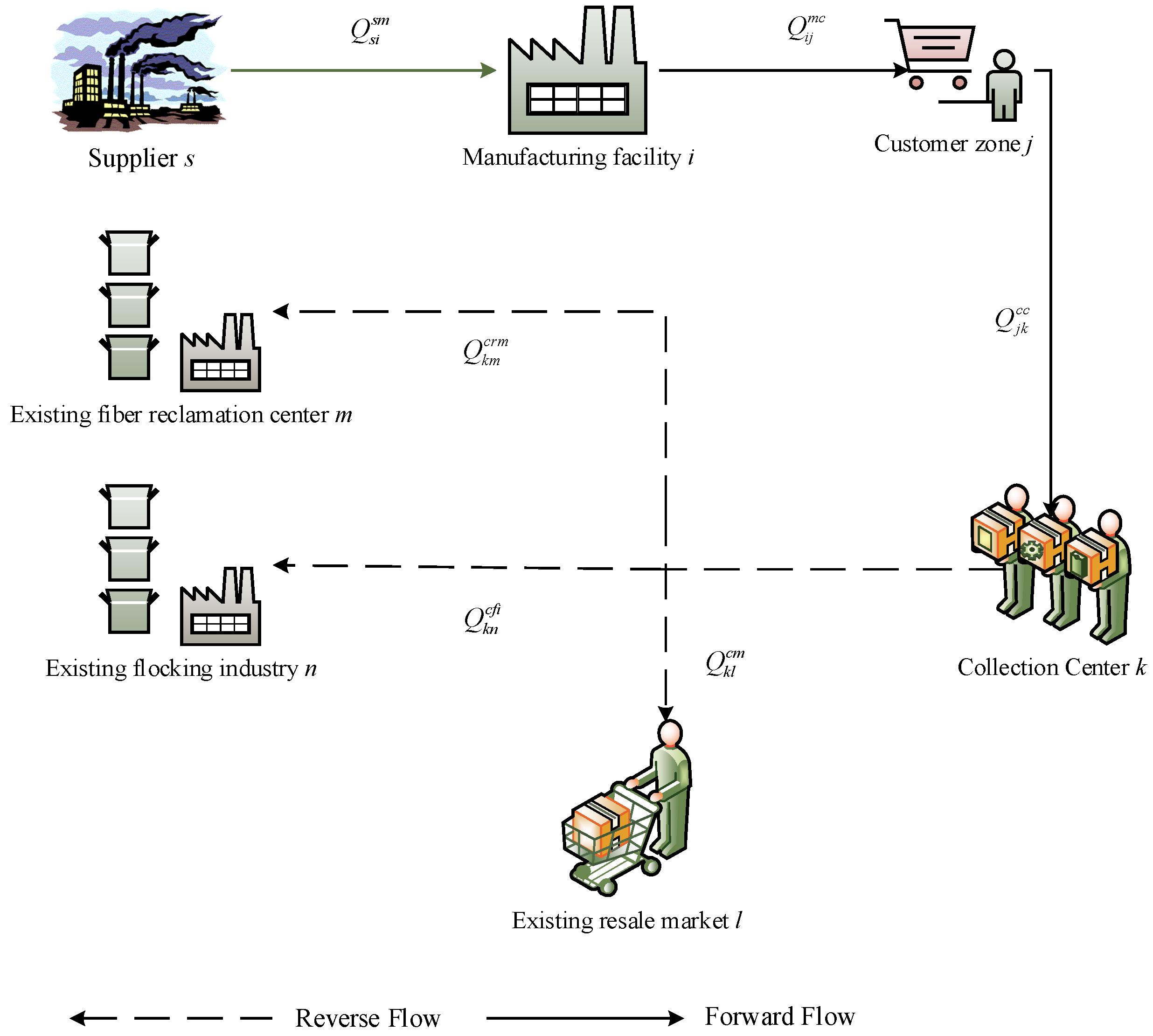
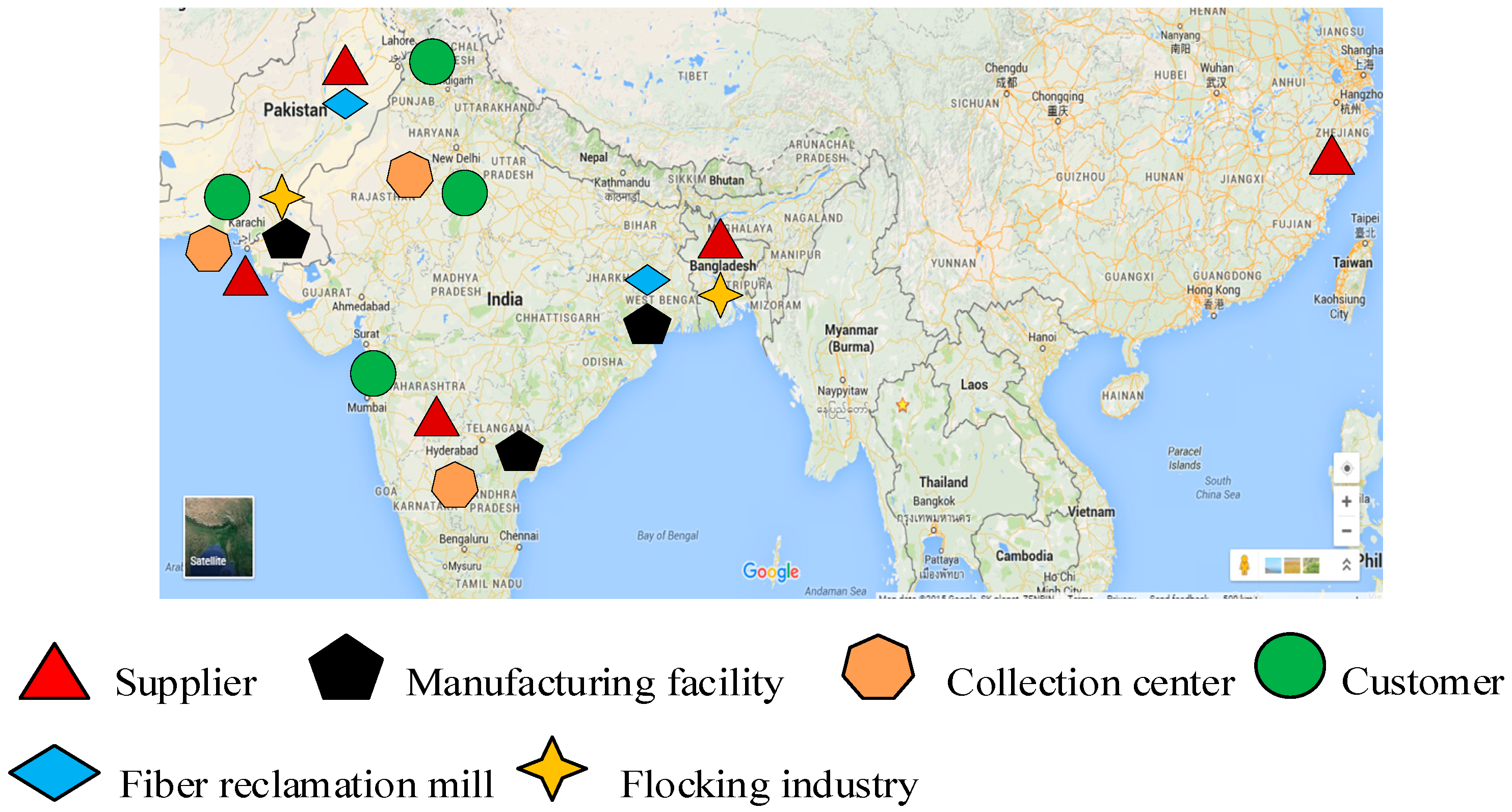
The problem is structured as a supply chain network (see
Figure 1) consisting of a set of suppliers (
s), from which various raw materials are purchased by a set of manufacturing facilities (
i), where the product is manufactured and distributed to various customer zones (
j). Collection centers (
k) are required to be opened to collect and process used products. The used products are then sent to either resale markets (
l) for selling or donating into poor countries, reclamation mills (
m) or flocking industry (
n) to recycle the used products that are not reusable.
After designing the structure of the supply chain problem, a multi-objective mixed integer linear programming (MOMILP) model is presented. The model consists of three objective functions and constraints related to the garment supply chain network under consideration. The notations and estimations of objective functions and constraints are discussed below.
2.1. Model Notations
| Indices |
| i | Index of potential location for manufacturing facilities i = 1, 2, …, I |
| j | Index of existing customer zones j = 1, 2, …, J |
| k | Index of potential locations for collection centers k = 1, 2, …, K |
| l | Index of existing markets to sale reusable textile l = 1, 2, …, L |
| m | Index of existing fiber reclamation mills m = 1, 2, …, M |
| n | Index of existing flocking industry n = 1, 2, …, N |
| s | Index of existing suppliers s = 1, 2, …, S |
| t | Index of time period t = 1, 2, …, T |
| Parameters |
| Demand for new product at customer zone j in period t (units/period) |
| Price of new product in period t ($/unit/period) |
| Percentage of products recovered from customer zone j in period t |
| Cost of installing manufacturing facility i ($) |
| Cost of installing collection center k ($) |
| Transportation cost per unit from supplier s to manufacturing facility i in period t ($/unit/period) |
| Transportation cost per unit from manufacturing facility i to customer zone j in period t ($/unit/period) |
| Transportation cost per unit from customer zone j to collection center k in period t ($/unit/period) |
| Transportation cost per unit from collection center k to resale market l in period t ($/unit/period) |
| Transportation cost per unit from collection center k to fiber reclamation mill m in period t ($/unit/period) |
| Transportation cost per unit from collection center k to flocking industry n in period t ($/unit/period) |
| Embodied carbon footprints of material coming from supplier s in period t (KgCO2/unit/period) |
| Carbon emission during production of unit product at manufacturing facility i in period t (KgCO2/unit/period) |
| Carbon emission for shipping unit product from supplier s to manufacturing facility i in period t (KgCO2/unit/period) |
| Carbon emission for shipping unit product from manufacturing facility i to customer zone j in period t (KgCO2/unit/period) |
| Carbon emission for shipping unit product from customer zone j to collection center k in period t (KgCO2/unit/period) |
| Carbon emission for shipping unit product from collection center k to resale market l in period t (KgCO2/unit/period) |
| Carbon emission for shipping unit product from collection center k to fiber reclamation mill m in period t (KgCO2/unit/period) |
| Carbon emission for shipping unit product from collection center k to flocking industry n in period t (KgCO2/unit/period) |
| Carbon emission during processing unit product at collection center k in period t (KgCO2/unit/period) |
| Carbon emission during processing unit product at fiber reclamation mill m in period t (KgCO2/unit/period) |
| Carbon emission during processing unit product at flocking industry n in period t (KgCO2/unit/period) |
| Unit purchase cost of material from supplier s in period t ($/unit/period) |
| Manufacturing cost per product at manufacturing facility i in period t ($/unit/period) |
| Processing cost per product at collection center k in period t ($/unit/period) |
| Processing cost per product at fiber reclamation mill m in period t ($/unit/period) |
| Processing cost per product at flocking industry n in period t ($/unit/period) |
| Capacity of manufacturing facility i in period t (units/period) |
| Capacity of collection center k in period t (units/period) |
| Capacity of fiber reclamation mill m in period t (units/period) |
| Capacity of flocking industry n in period t (units/period) |
| Capacity of supplier s in period t (units/period) |
| Probability of disruption risk at supplier s in period t |
| Probability of disruption risk at manufacturing facility i in period t |
| Probability of disruption risk at collection center k in period t |
| Decision Variables |
| Transportation quantity from supplier s to manufacturing facility i in period t (units/period) |
| Transportation quantity from manufacturing facility i to customer zone j in period t (units/period) |
| Transportation quantity from customer zone j to collection center k in period t (units/period) |
| Transportation quantity from collection center k to resale market l in period t (units/period) |
| Transportation quantity from collection center k to fiber reclamation mill m in period t (units/period) |
| Transportation quantity from collection center k to flocking industry n in period t (units/period) |
| If a manufacturing facility i is open 1, otherwise 0 |
| If a collection center k is open 1, otherwise 0 |
2.2. Formulation of Objective Functions
The objective of the proposed sustainable and resilient supply chain model is to minimize the total supply chain cost, minimize carbon emission, and minimize expected disruption cost in all considered periods. First, objective function fcost in Equation (1) minimizes the total cost of supply chain. Second, objective function fsus in Equation (2) minimizes the total carbon emission. Third, objective function fedc in Equation (3) minimizes expected disruption cost. Various estimations related to these objectives are discussed in below section.
a. Total supply chain cost (Economic objective)
Various costs associated with the supply chain are calculated in Equation (4). The first two terms represent the installation cost of manufacturing facilities and collection centers, respectively. The remaining terms represent the material purchasing cost, production cost, and processing costs for suppliers, manufacturing facilities, collection centers, fiber reclamation center, and flocking industries along with corresponding transportation costs in all periods, respectively.
b. Total Carbon emission (Sustainable objective)
Various carbon emissions in the supply chain are computed in Equation (5). The first term estimates embodied carbon footprints and carbon emission during transportation of material coming from various suppliers. It is very important to minimize the embodied carbon footprint of the procured material in order to consider every aspect of sustainable supply chain. For instance, if the manufacturer unit available in highly green zone procured raw material with a high carbon embodied footprint, will fail to attain its sustainability objective and may face legal restriction because of being in the green zone. Second term includes carbon emission during production and transportation of product to customer zones. Third term includes carbon emission during processes and collection centers and transportation of used products. Fourth term includes carbon emission during transportation of used products to resale markets. The last two terms include carbon emission during recycling processes and transportation of used products from collection centers to recycling centers.
c. Expected disruption cost (Resilience objective)
The goal of this objective is to minimize expected disruption cost due to any disruption risk associated with any member of the supply chain in all periods. In this research, only the forward supply chain is considered to measure the resilience objective since the forward supply chain resiliency is more important and also has an impact on the reverse supply chain. Hence, Equation (6) measures the expected disruption cost due to disruption of the supplier, manufacturing facilities, and collection centers in all periods.
2.3. Formulation of Constraints
Constraints (7)–(11) are capacity restrictions on supplier, manufacturing facilities, collection center, fiber reclamation mill, and flocking industry, respectively, in all periods. In addition, Constraints (8) and (9) ensure that the products are produced and processed only on existing manufacturing facilities and collection centers respectively in all periods.
Constraint (12) promises that the amount of products transported from manufacturing facilities to customer zone
j should satisfy its demand. Constraint (13) shows that all the used products are collected from customer zones.
Constraint (14) balances the input and output of the material in a manufacturing facility. The amount of incoming material from suppliers to the manufacturing facility is equal to a number of outgoing products from the manufacturing facility to the customer zone. Similarly, Constraints (15)–(17) balance the input and output of used products in the collection center. The incoming used products from customer zones are either sent to resale markets or separated for fiber reclamation process and flocking process. It is assumed in this study that 50% of collected products are reusable, and the remaining products are then separated for reclamation and flocking processes. According to U.K. industry sources, about 50 percent of collected textile items can be reused and the remaining 50 percent can recycled [
13].
Constraints (18) and (19) impose non-negativity and binary restrictions to all the corresponding decision variables, respectively.
3. Proposed Solution Methodology
Several solution methodologies are developed to solve the multi-objective programming models. Fuzzy-based programming techniques are highly used in this area because of their capability in estimation and adjustment of the decision maker’s satisfaction level of each objective explicitly [
14]. In this study, initially, the methodology proposed by Jiménez, et al. [
15] is applied to convert the uncertain model into an equivalent auxiliary crisp model. The proposed uncertain model in previous section assumes possibilistic fuzzy parameters. Then the interactive fuzzy weight, based solution methodology, is developed to solve the proposed sustainable and resilient supply chain model. The steps of the proposed solution methodology are summarized as follows:
Step 1. Convert fuzzy multi-objective model into equivalent auxiliary crisp model
In this stage, the proposed multi-objective model is converted into an equivalent auxiliary crisp model. Jiménez, Arenas, Bilbao and Rodrı [
15] method used in this study due to: (i) its strong mathematical formation which is based on expected interval and expected value of fuzzy numbers to deal with uncertain parameters; and (ii) its support of any fuzzy membership function such as trapezoidal and triangular with either symmetric or asymmetric forms. Readers can refer Jiménez, Arenas, Bilbao and Rodrı [
15] for detail information on this method.
Assume that “
” is a triangular fuzzy number, then the membership function of
can be defined as in Equation (20), where
pes is the pessimistic value,
mos is the most likely value, and
opt is the optimistic value of triangular fuzzy number.
According to Jiménez, Arenas, Bilbao and Rodrı [
15], the expected interval (EI) and expected value (EV) of triangular fuzzy number
can be defined as follows.
Consequently, using the definition of expected interval and expected value of a fuzzy number, the equivalent auxiliary crisp model of a proposed possibilistic sustainable and resilient supply chain model can be formulated as follows. The uncertain objective functions are converted into crisp forms using expected value definition. In addition, the uncertain constraints will be converted into equivalent crisp forms using expected interval definition. Where, α represents the confidence level. The decision makers can choose level of confidence based on available information and their perception. Additionally, decision makers can vary value of α in order to generate different tradeoff solutions. In this formulation, α = 0.5 means that the most likely values of parameters are preferred, whereas α < 0.5 means model parameter values are between pessimistic and most likely values. Similarly, α > 0.5 means that value of model parameters are between most likely and pessimistic values.
Step 2. Obtain efficient α-extreme solutions
Usually, two methods are used in practice to find out efficient α-extreme solutions. In the first method, the DMs are encouraged to suggest the bounds on each objective. However, this method is less common because it is difficult for DMs to suggest bounds when the problem is of large scale. The second method that we used in this study is to find an extreme possible solution by solving each objective separately. In this step, the crisp model is solved considering one objective along with constraints in a single run. This results in lower (α-LB) and upper (α-UB) bounds on each objective function.
Step 3. Determine the Fuzzy membership function for each objective
The payoff values (i.e., α-LB and α-UB) are now used to develop the fuzzy membership function for each objective of proposed model. Assuming that membership functions based on preference or satisfaction are linear, the linear membership for fuzzy objectives is given as follows:
where
,
, and
are satisfaction level of cost, sustainability, and resilience objectives, respectively.
Step 4. Convert multi-objective model into single objective
Various interactive approaches are proposed to solve multi-objective problems. Selection of a suitable solution methodology for a certain multi-objective optimization problem is not easy, as has been made abundantly clear [
16]. In this study, the fuzzy linguistic weight-based method is proposed by improving Werner’s “fuzzy and” operator method [
17]. The proposed method takes advantage of both Werner’s and the fuzzy-weighted method. The detail of proposed method is given as follows.
In practice, DMs feel comfortable assigning importance of objectives in linguistic terms. In this proposed method, the fuzzy linguistic variables are suggested to assign the importance of objectives.
Table 1 shows the five-scale importance level as triangular fuzzy number adopted from Wang and Lee [
18]. Suppose that decision-making panel consists of
n DMs, then the importance of objectives can be estimated as follows.
- (1)
Set the linguistic variables for the importance of objectives.
- (2)
Evaluate the importance of objectives based on linguistic variables from
Table 1.
- (3)
Aggregate each of the fuzzy number using
where
AFNq is aggregate fuzzy number of
qth objective and (
) is
nth decision maker perception of importance for
qth objective.
- (4)
Estimate the fuzzy weight of
qth objective as shown below.
where
=
AFNq, q = 1, 2, 3 number of objectives.
- (5)
Calculate the normalized fuzzy weights of objectives by:
- (6)
Finally, the single objective model using improved Werner’s method can be formed as below.
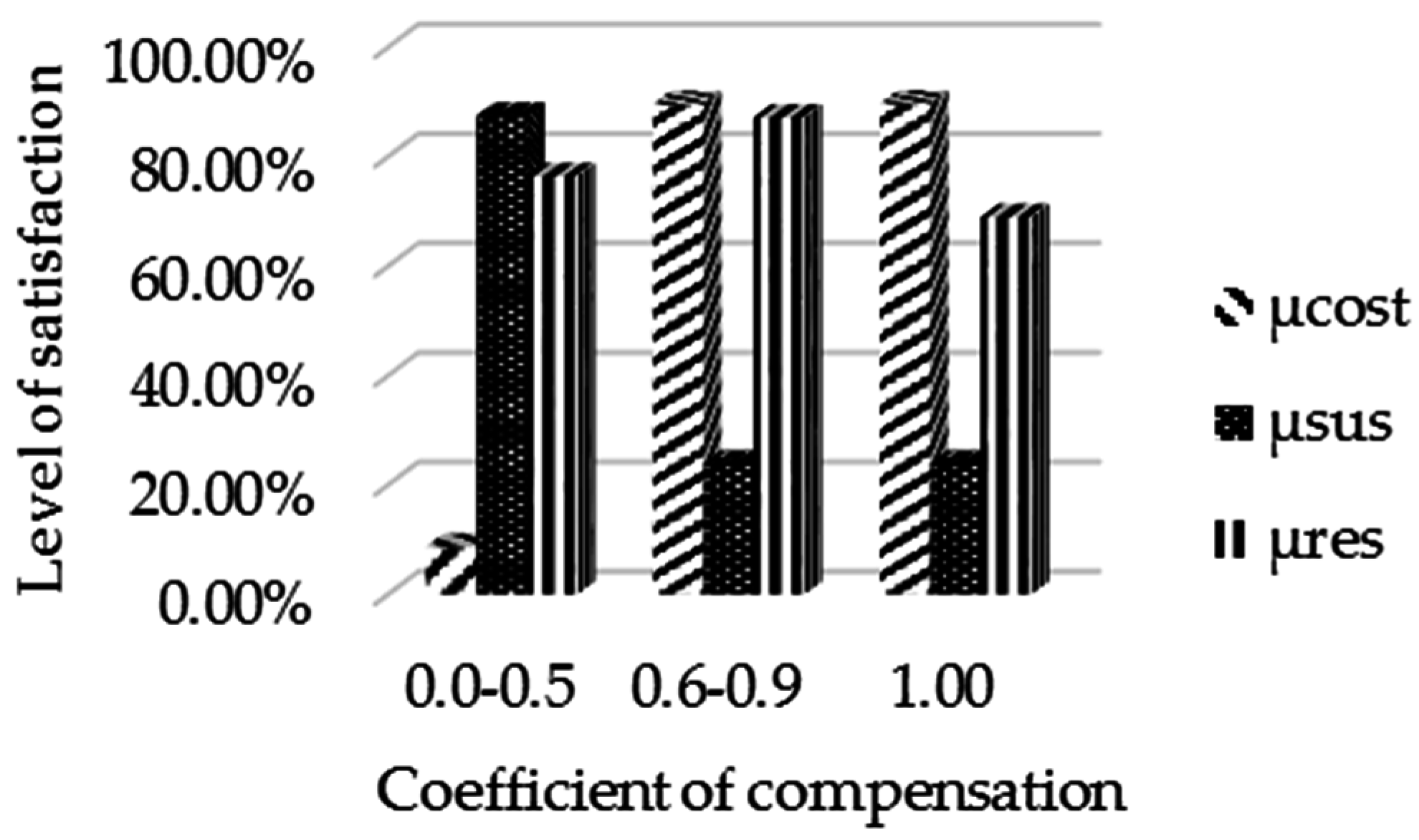
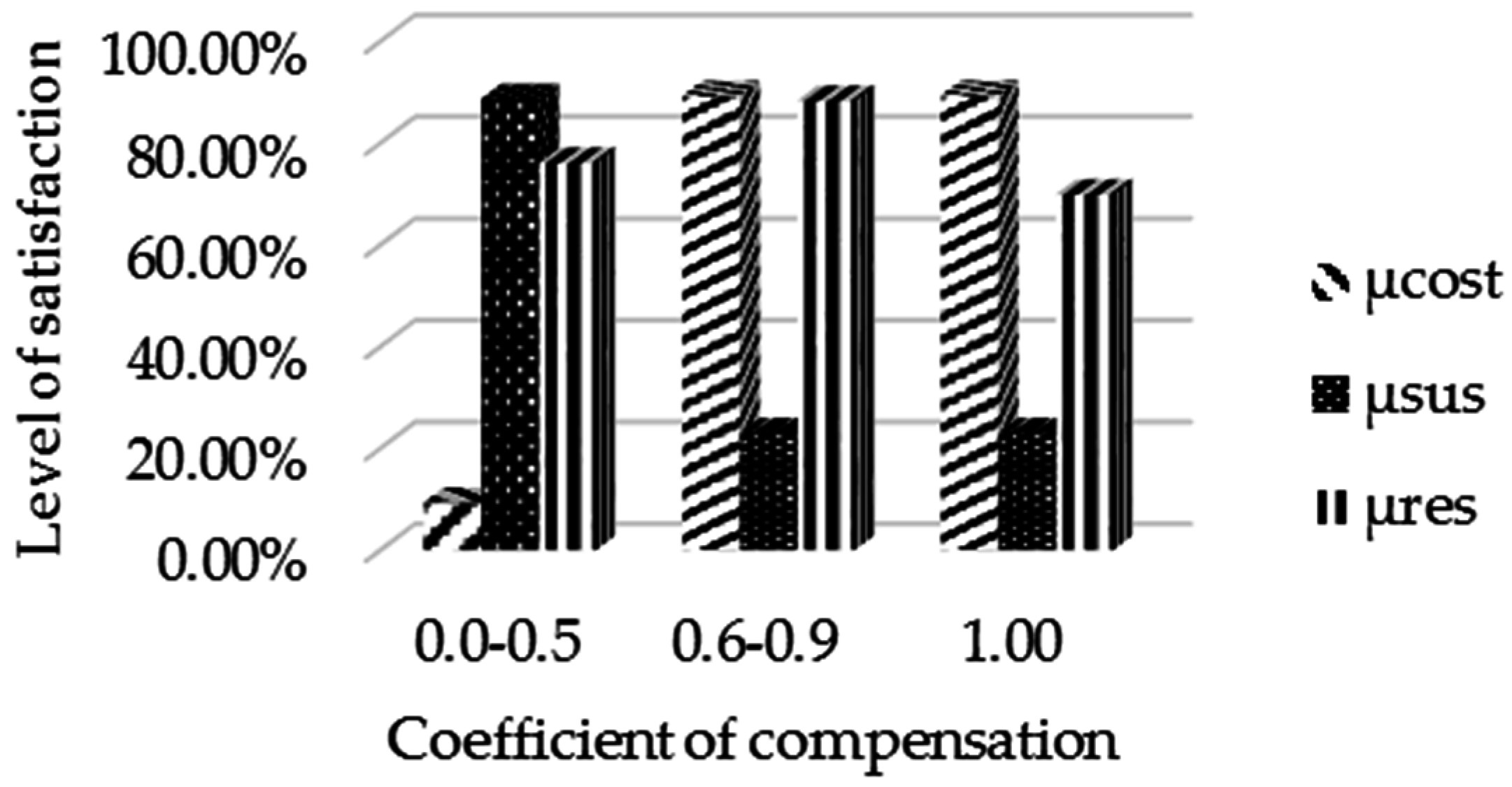
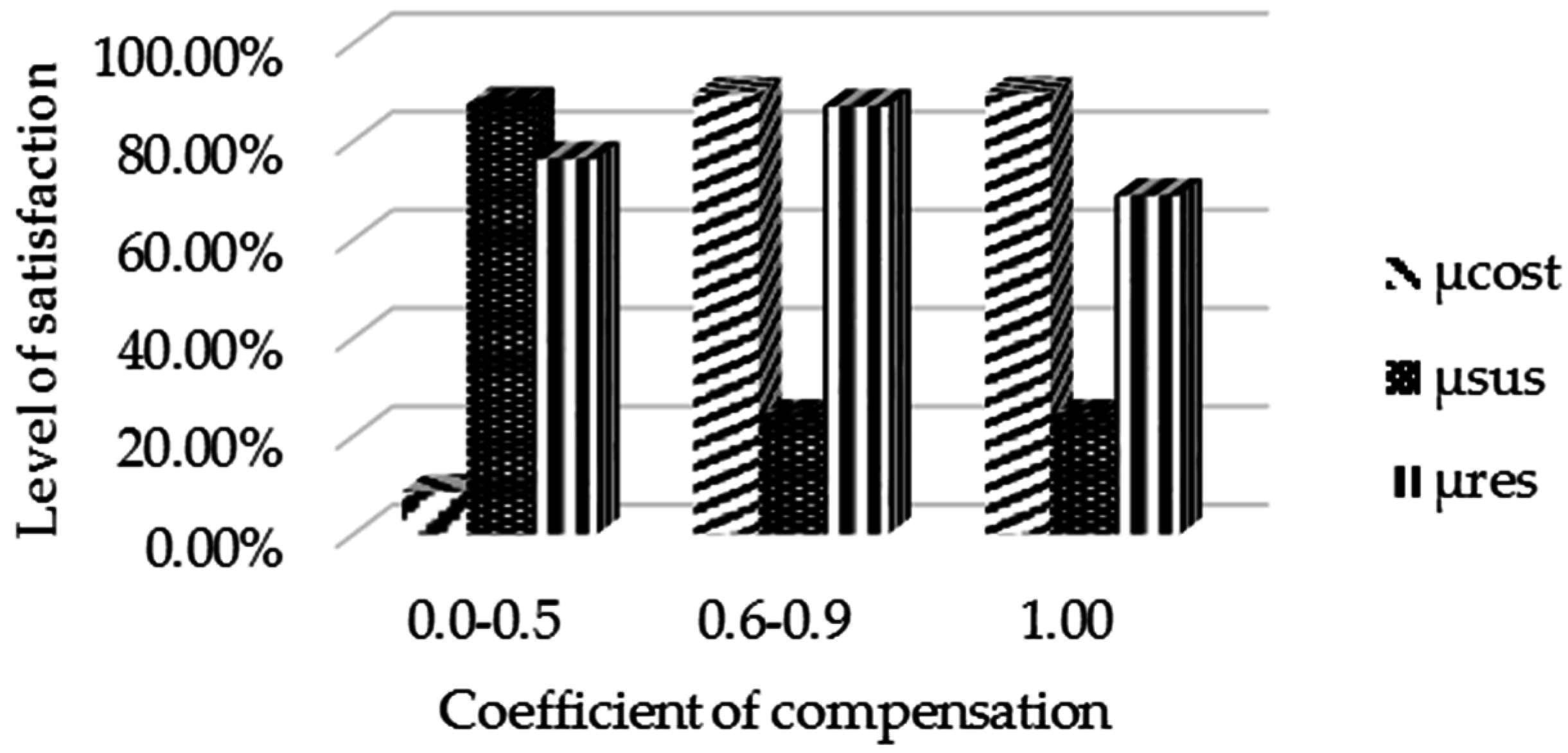
where, θ denotes the coefficient of compensation and ζ1, ζ2, and ζ3 are the difference between satisfaction level of objectives with their minimum satisfaction level. That is, ζ1 = µcost – ζ0, ζ2 = µsus – ζ0, and ζ3 = µres – ζ0. and are the normalized weights for cost, sustainability, and resilience objectives, respectively.
Step 5. Determine the solution method parameters
To solve the mathematical models developed in Step 4, the values of coefficient of compensation (θ) and relative importance of objectives () are determined.
Step 6. Solve the model
The mathematical models developed in Step 4 are solved using required model and solution methodology parameters. If decision makers are not satisfied with the results, they can provide another solution by modifying the solution method parameters (i.e., θ and ). If decision makers want to modify value of α, then they must restart the process at Step 2.
4. Numerical Example
In the case when real data are not available, a test problem is developed based on a hypothetical supply chain, where data are conducted based on reasonable assumptions and several public resources. In real life implementation, required data can be obtained from various sources, such as installation and production costs can be obtained from already present manufacturing facilities. Transportation costs between facilities can easily be obtained from available transportation services. In this example, supply chain risk is estimated by using resilience index as discussed above. To solve the proposed model, a garment supply chain is chosen, which consists of five potential suppliers, three manufacturing facilities, four customer zones, three collection centers, two resale markets, two flocking industries, and two reclamation mills, as shown in
Figure 2. This numercial example assumes that the supply chain is producing single garment product i.e., jeans.
The presented supply chain included five suppliers located at Karachi and Faisalabad cities of Pakistan, Hyderabad city of India, Dhaka city of Bangladesh, and Shaoxing city of China. Three potential locations of manufacturing facilities are located in Karachi, Pakistan, Hyderabad, India, and Kolkata, India. Four customer zones are chosen to sell the product located in Karachi, Pakistan, Lahore, Pakistan, Mumbai, India, and Delhi, India. Karachi, Pakistan, Delhi, India, and Hyderabad, India are selected for locations of collection centers. Mali and Libya are selected as resale markets. Potential locations of flocking industries are located at Karachi, Pakistan and Dhaka, Bangladesh, whereas, potential reclamation mills are located at Kolkata, India and Faisalabad, Pakistan. The decisions that have to be made here are following:
A number of manufacturing facilities required to open and their locations.
The amount of products produced at each opened facility and which customer zones satisfied from each opened facility.
Suppliers selected for supplying material to each opened manufacturing facility.
Quantity of material to be purchased from each selected supplier
Number and locations of collection centers opened.
Location of recycling facilities (i.e., flocking industry and reclamation mill) preferred for recycling used products.
Location of resale market and quantity of products that can be resale to these markets.
4.1. Data population
The collection of data was performed to solve the model and generate useful results. The triangular fuzzy parameters
are estimated by initially calculating the most likely
value of parameters. These most likely values of parameters were picked from various sources (such as SeaRates [
19] for transportation distances and costs and CargoRouter [
20] for CO
2 emissions) some reasonable assumptions were made, and all required calculations were done beforehand. Thereafter, two random numbers (
n1,
n2) are generated between 0.2 and 0.8 using uniform distribution and the pessimistic
and optimistic
values of fuzzy number
are estimated as follows.
All the required data (the most likely value) are presented in
Appendix A with sources (i.e., either official data or hypothetical data).
4.2. Result and Discussion
The crisp sustainable and resilient model is solved using α = 0.90 to obtain payoff values. Payoff values (i.e., α-LB and α-UB) of three objectives are shown in
Table 2.
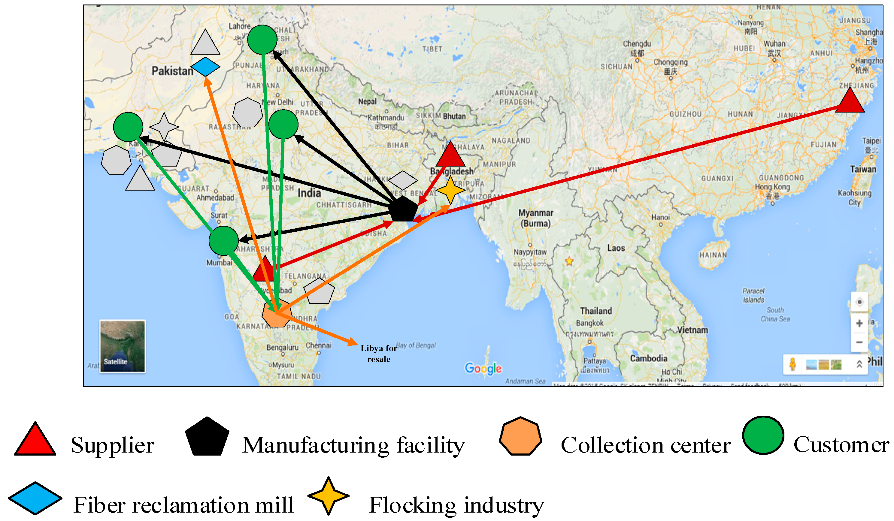
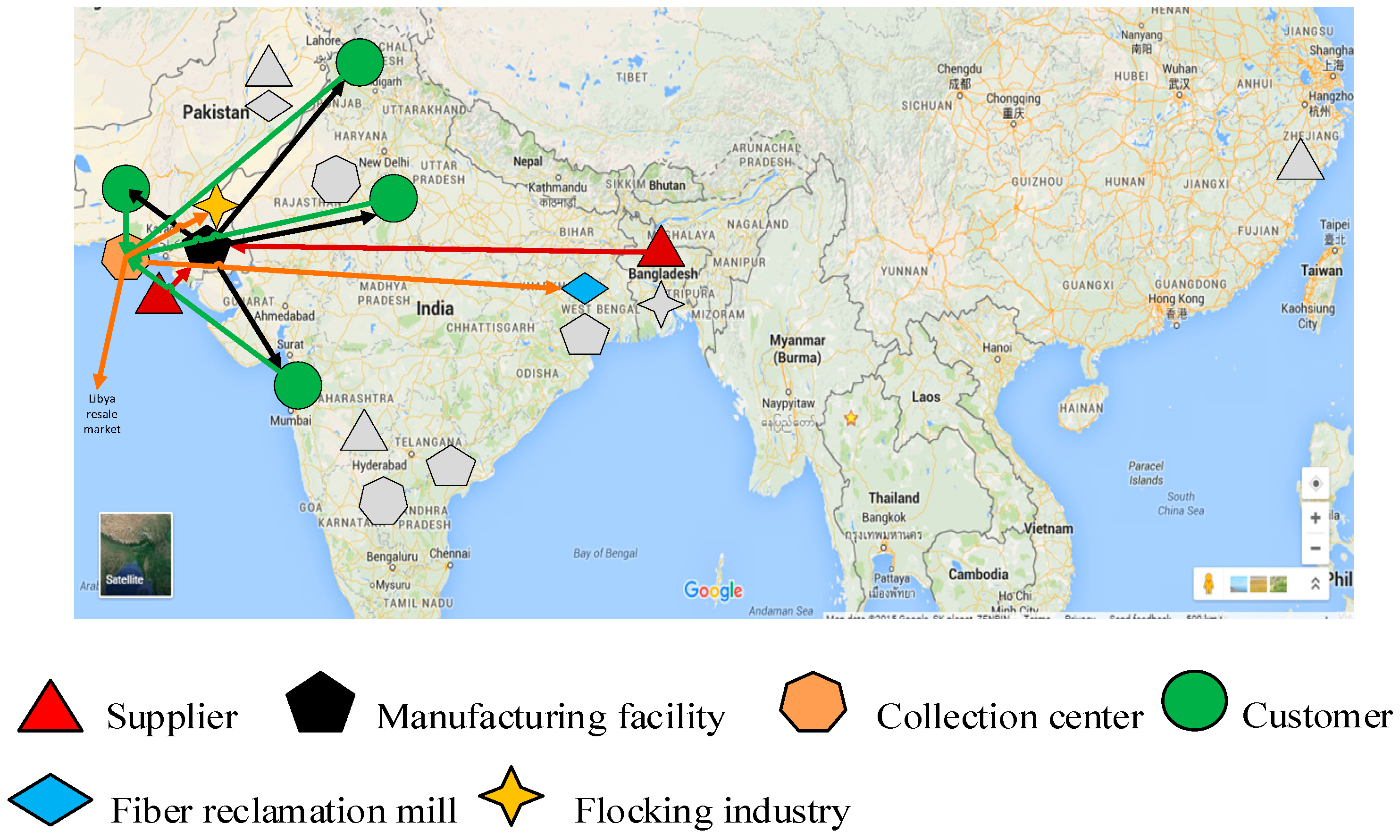
It can be seen from results that all three objectives, i.e., economic, sustainability, and resilience, of supply chain networks are conflicting in nature (see
Figure 3,
Figure 4 and
Figure 5). If an organization wants to consider the economic perspective, Kolkata is a suitable location for a manufacturing facility. On the other hand, Karachi is suitable location from sustainability perspective and Hyderabad is suitable location from resilience perspective. Similarly, based on procurement and transportation cost, suitable suppliers are located in Shaoxing, Dhaka, and Hyderabad. Alternatively, suppliers located at Karachi and Dhaka are suitable choices when sustainability objective is given priority over other objectives. Results show that suppliers with higher resilience index or lesser probability of disruptions are given priority when the resilience objective is considered. Similarly, manufacturing facility and collection centers are open in the highest resilience index locations. The resilience objective ensures that the supply chain network should consider disruption risks in advance. This minimizes the risk of dropping supply chain performance during a disruption event. The impact of disruption risks can be minimized by: (1) selecting suppliers based on their adopted resilience level and the probability of disruption risks in suppliers’ locations; (2) establishing manufacturing facilities, collection centers, and other service facilities to locations where the probability of disruption risks are low or resilience index score of location is high; (3) transporting minimum quantity of material form higher risk zones and vice versa; and (4) it is also found from this study that it is not a suitable choice to select key suppliers from the same region because this leads to higher supply density, which is vulnerable during high impact and low probability (HILP) risk events.
The second step of the proposed solution methodology is to develop fuzzy membership function. The fuzzy membership functions for satisfaction level of each objective are given below.
The proposed model is solved using developed Fuzzy weighted method and results are compared with Werner’s method (see
Table 3). Results of Werner’s method and proposed method show that the proposed method is more flexible as it also considered fuzzy importance level of objectives.
4.3. Sensitivity Analysis
The details of the sensitivity analysis of proposed solution method are given in
Table 4. The model is solved using the proposed fuzzy linguistic weight method by varying
α and
θ values.
Figure 6,
Figure 7 and
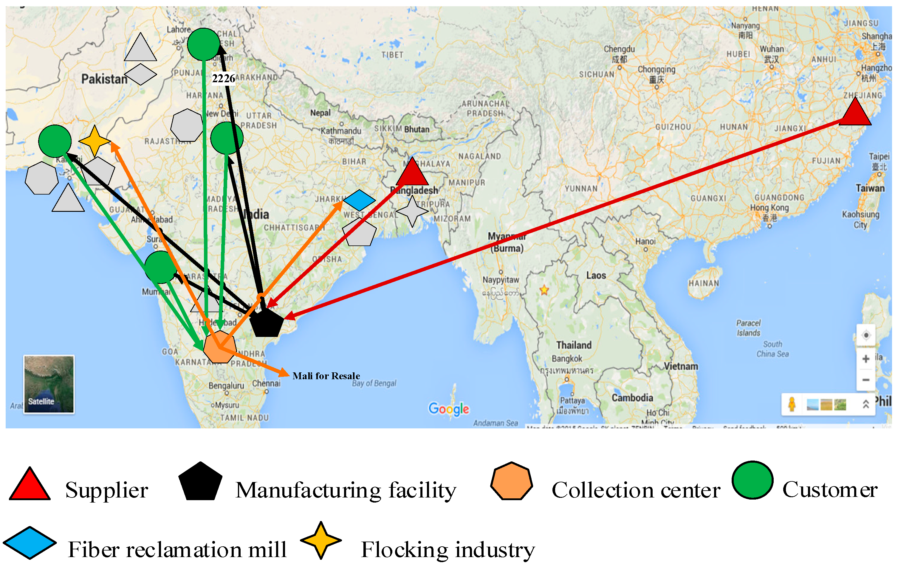
Figure 8 show the graphical representations of sensitivity analysis based on different α values, respectively. We assume that DMs reach a final solution at
α = 0.9 and
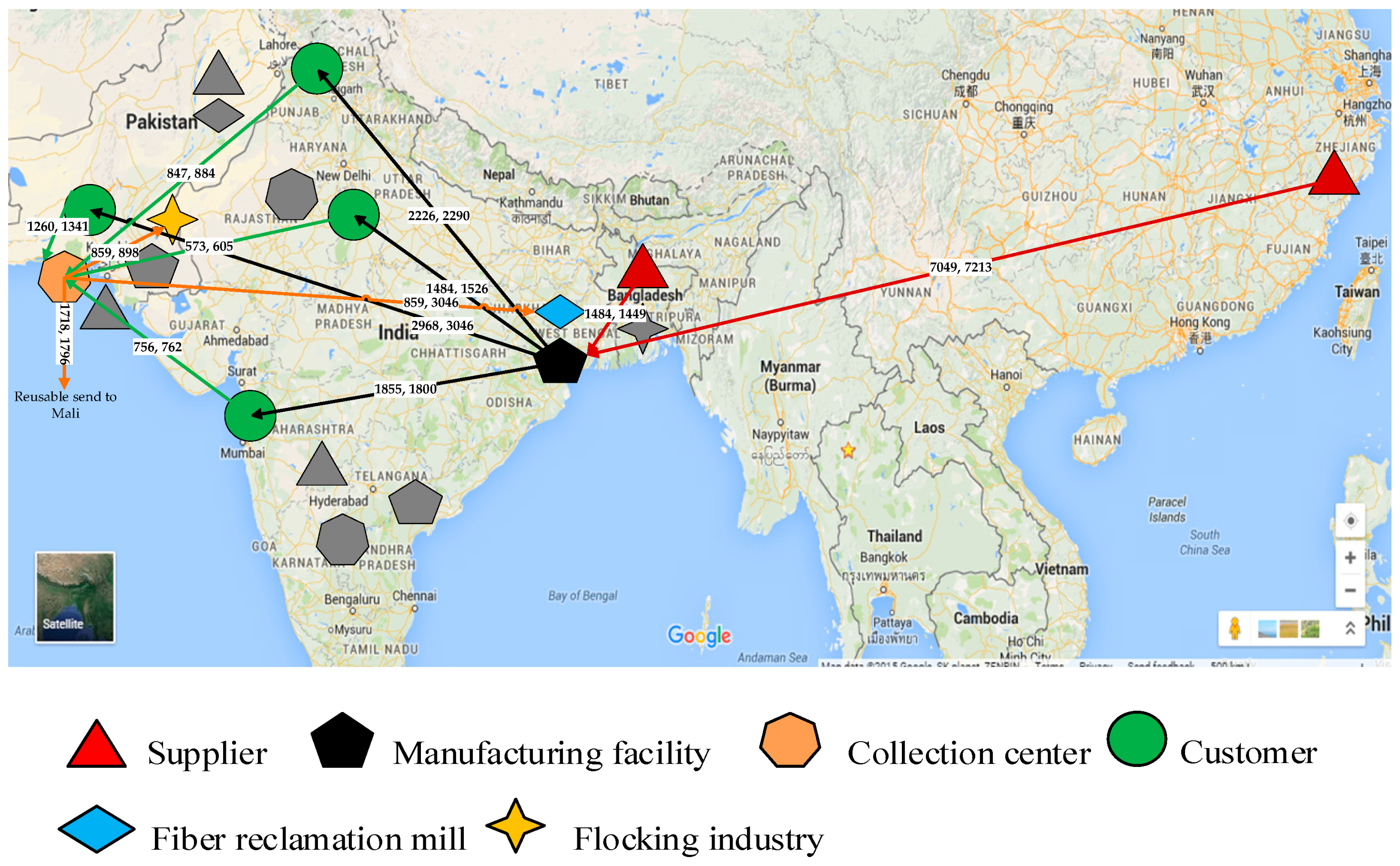
θ = 0.7–0.9 (highlighted row) based on DMs preferences, which results in a supply chain network as shown in
Figure 9. The final supply chain required to open a manufacturing facility in Kolkata and procure material from Shaoxing, China, and Dhaka suppliers. The optimal location for the collection center is Karachi where used products can be processed. The reusable products can be sent to Mali, Africa for donations. While the remaining used products will be sent to the flocking industry located at Karachi and reclamation mill located at Kolkata.
5. Conclusions
This study focuses on developing sustainable and resilience supply chain network by considering economic, green, and resilience paradigm of supply chain. The research proposed a possibilistic fuzzy multi-objective programming-based approach to handle conflicting objectives, such as supply chain costs, carbon emissions, and resilience. The significant contribution of this research is the inclusion of a resilience factor based on Resilience Index, a data driven tool in the design of the sustainable supply chain network by considering nine major supply chain risks. Furthermore, a fuzzy-weighted Werner’s interactive method based solution methodology is proposed to solve a possibilistic fuzzy multi-objective model. Thus, the mathematical model and solution methodology can provide a quality solution to decision makers. It is found from this research that disruption risks create chaotic situations for managers and managing shortages are a priority for them. During these disruption risks, managers try to use alternate sources to minimize shortages and losses, this decision leads to decline in sustainable performance due to possible increment in: (1) embodied carbon footprints; (2) transportation CO2 emission; and (3) economic losses.
As this is the primary work of developing sustainable and resilient supply chain network design under stochastic and recognitive uncertainties using a possibilistic fuzzy programming approach, many possible future research avenues can be defined in this context. For example, this research utilizes the concept of expected disruption cost to measure resilience in supply chain network; it will be valuable to consider other measures such as supply chain density and node criticality as the objective function. Furthermore, real-time GIS data can be utilized to calculate the probability disruption risks in various regions. The model can also be extended by incorporating different transportation modes and to consider road restrictions, for example, heavy trucks may not enter some roads.


