Sustainable Mobility: Longitudinal Analysis of Built Environment on Transit Ridership

Abstract

Given the concerns about urban mobility, traffic congestion, and greenhouse gas (GHG) emissions, extensive research has explored the relationship between the built environment and transit ridership. However, the nature of aggregation and the cross-sectional approach of the research rarely provide essential clues on the potential of a transit system as a sustainable mobility option. From the perspective of longitudinal sustainability, this paper develops regression models for rail transit stations in the Los Angeles Metro system. These models attempt to identify the socio-demographic characteristics and land use features influencing longitudinal transit ridership changes. Step-wise ordinary least square (OLS) regression models are used to identify factors that contribute to transit ridership changes. Those factors include the number of dwelling units, employment-oriented land uses such as office and commercial land uses, and land use balance. The models suggest a negative relationship between job and population balance with transit ridership change. They also raise a question regarding the 0.4 km radius commonly used in transit analysis. The models indicate that the 0.4 km radius is too small to capture the significant influence of the built environment on transit ridership.

1. Introduction

Urban mobility, defined as the movement of people or goods, is a key factor in supporting residents and businesses to manage their everyday life and tasks. It is clear that transportation services must satisfy the demand from businesses and residents that they are increasingly convenient, fast and predictable. The private vehicle is one of most important mobility options for daily urban mobility in the U.S. According to 2009 National Household Travel Survey, private vehicles account for 83% of all person trips in the U.S. However, private vehicles are one of the main sources of greenhouse gas (GHG) emissions in the U.S. About 26% of greenhouse gas in the U.S. is emitted by transportation activity, and 81% of this transportation greenhouse gas is produced from passenger cars, light trucks, and heavy duty vehicles in 2014 [1].

Taking consideration of the negative aspects of private vehicle such as congestion, policy makers are becoming more concerned about the sustainability of their mode of travel and are seeking the successful introduction and rapid penetration of sustainable mobility services. A model of sustainable mobility would be one where the means of transport consumes the least energy and produces less pollution per passenger mile traveled (PMT). Sustainable mobility does not intend to achieve environmental goals (i.e., a reduction of greenhouse gas (GHG) emissions) by reducing mobility. It attempts to identify alternative solutions that reduce GHG emissions while increasing mobility for residents, especially people who have less flexibility in their mode choice [2]. This emphasizes the roles of sustainable mobility for social sustainability. The social aspects of sustainable mobility connect mobility options with broader social concerns like equity and public health.

In this sense, public transit is a perfect example of a sustainable mobility option due to its environmental benefits as well as its carrying capacity [3]. Considerable research emphasizes the promotion of bus transit services for disadvantaged communities from the perspective of social justice [4,5]. Therefore, considerable research addresses the strategies that promote public transit ridership. While some research suggests the system innovation and adaptation of new technologies including fuel cell vehicles [6], fuel-efficient three wheeled cars [7], and standardized vehicle designs [8], various other authors emphasize transportation planning and policy strategies. These strategies include Transit-Oriented Development (TOD) and Smart Growth. Extensive transportation literature also supports the strategies emphasizing urban density, mixed-use development, and pedestrian and bicycle friendly environments around transit stations [9,10]. The literature has provided important insights into the direct relationship between the built environment and transit ridership. However, a large body of the literature analyzes the relationship employing a cross-sectional approach that rarely provides crucial clues to the potential of transit systems for long-term sustainability.

The purpose of this paper is to shed light on the factors contributing to the change of transit ridership from the perspective of sustainability. Focusing on the Los Angeles Metro rail transit lines, this paper particularly identifies land use features and socio-demographic characteristics within a transit catchment area that contribute to longitudinal transit ridership changes. It investigates the longitudinal impacts of the contributing factors on the changes of rail transit ridership by conducting a step-wise ordinary least square (OLS) regression analysis. By re-assessing the factors included in cross-sectional studies with a longitudinal perspective, the findings from the analysis provide a better understanding of the factors contributing to the sustainability of a transit system.

2. Literature Review

A large body of literature has documented factors that affect transit ridership at the aggregate level. Depending on the control of the transit system, candidates can generally be categorized into two types: external factors related to the transit demand side and internal factors representing the transit supply side [11,12]. External factors include socio-economic factors (e.g., population characteristics and the metropolitan economy), spatial factors (e.g., the built environment), alternative travel modes (e.g., highway accessibility, fuel prices, and parking availability), and public funding (e.g., transit subsidies) [13]. In contrast to the external factors, internal factors are normally under the control of the transit system and management, including transit fares, service quantity (e.g., headways, route coverage, and revenue) and service quality (e.g., on-street service, service safety, reliability, and comfort) [14,15,16].

Findings from these studies indicate that some factors have a significant impact on ridership as expected, but that others are mixed. For example, not surprisingly, the level of income has a negative influence on transit ridership [17,18]. Evidence consistently supports the finding that car ownership, parking costs, and the availability of parking space are significantly related to transit use with the expected signs [19]. However, the influence of gas prices is slightly mixed. One study revealed a small or minor impact of fuel prices [20], but another found that the gasoline price has the largest impact on transit ridership [21].

Depending on the geographic scale by which transit ridership is measured, empirical studies connecting land use and transit ridership can be divided into two groups: macro and micro scale. A number of macro-level studies covering metropolitan statistical areas (MSAs), urbanized areas, counties, and cities have focused on the relative importance of urban structure and transit service in explaining the variation in transit ridership [11,21,22]. More specifically, some scholars argue that transit ridership is tied to the strength of the central business district (CBD) in terms of population and employment, acknowledging that the decline in ridership is attributable to the growth of decentralized employment and scattered residential areas [13]. Other scholars put more stress on the importance of the transit service system which better connects dispersed employment centers and residential areas, arguing against the relevance of urban structure to transit ridership [23,24].

At the micro-level, considerable attention in studies has been paid not only to the capability of physical configurations to promote the level of transit use, but also to the impact of TOD projects on ridership [9,13,16,25]. In terms of the role of environmental factors, it is generally assumed that transit use is higher in more dense, diverse, and walkable urban environments [26]. Dense, diverse land use patterns around rail transit stations are one of the primary factors that guarantee successful strategic planning for railway stations and sustainable transit system [27,28]. It is important to focus on the land use conditions of the site within which the transit station functions at the first step of transit system development process. Proponents of Smart Growth and TOD strategies argue that those physical configurations increase transit ridership by providing easy, convenient access to transit systems a short distance from the origin/destination, with high concentrations of activity and well-connected street patterns [26]. Along with the single effect of density, Cervero reported that high density brings more transit ridership when it is accompanied by a mix of residential, commercial, and office uses in proximity to the station. Studies also conclude that a pedestrian-friendly environment around stations substantially improves the accessibility to the transit system by foot or bicycle [10].

However, it is difficult to accept that the pedestrian-friendly environment itself leads to the significant increase in transit ridership. The reasoning is that people who use transit are not limited to walkers, and that a pedestrian-friendly environment does not necessarily result in a transit friendly environment. It appears more persuasive to conclude that, to some degree, the role of physical environmental factors around transit service areas is fairly significant, but its magnitude is relatively marginal when compared with internal factors including socio-economic conditions [10,23].

In summary, a large body of literature has documented the relationship between the built environment and transit use. However, given the nature of aggregation and the cross-sectional approach, the causality and self-selection issue still remains unanswered. In other words, aggregate data often mask important but unobserved variance within a group, lacking individual information on the preference for public transit as well as residential location choice. Cross-sectional approaches rarely provide crucial clues to the sustainability of the transit system for long periods since they only consider one point in time. Several studies at the macro level have incorporated longitudinal data to explore whether the change in urban structure can lead to a change in transit ridership [29]. However, there are limited studies that attempt to investigate the relationship between the change in micro-scale land use patterns and the change in transit ridership. This paper attempts to fill this research gap by detecting historical parcel-level land use changes as well as socio-demographic factors around transit catchment areas and associating the factors with longitudinal transit ridership trends.

3. Methodology

3.1. Study Area

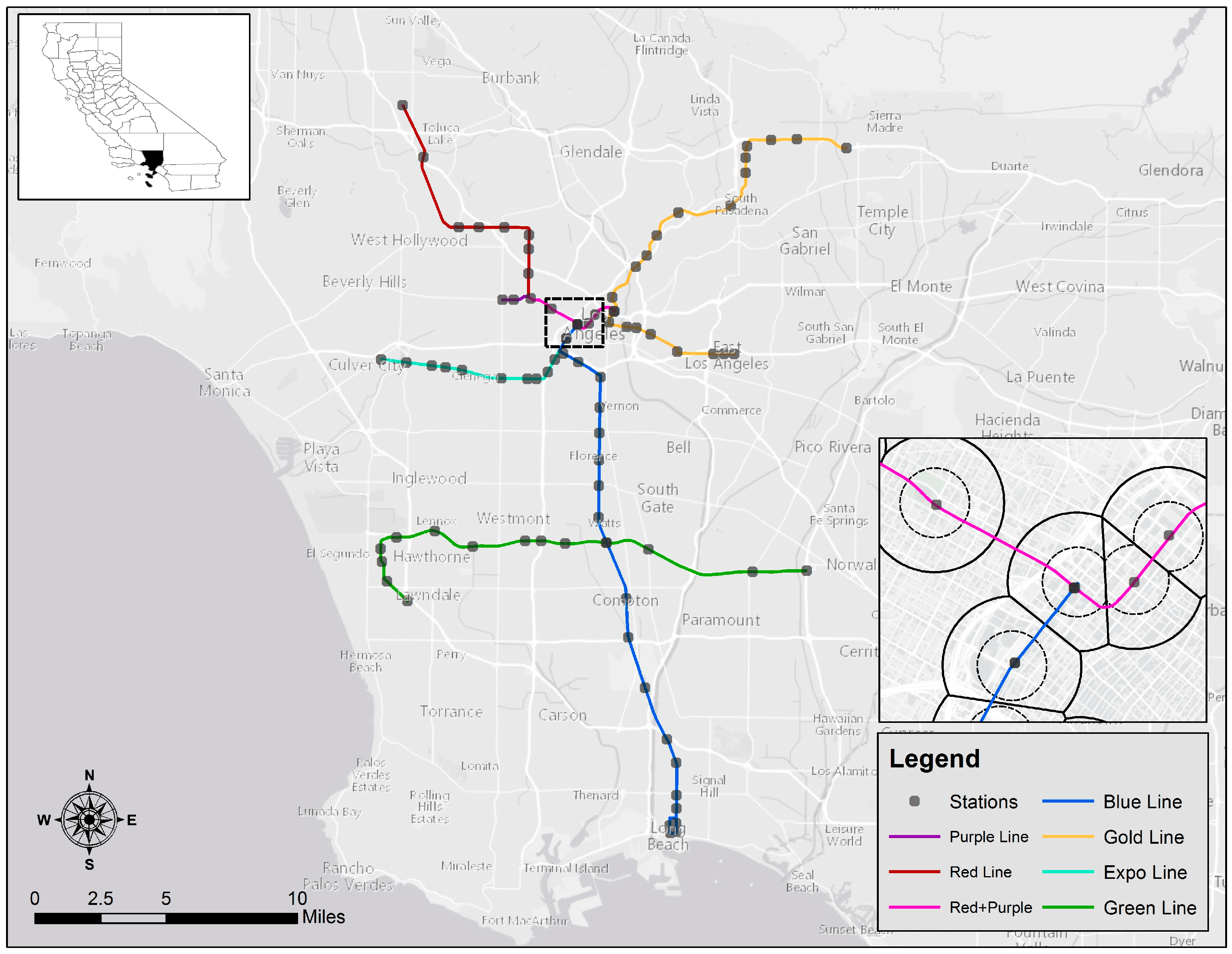
The geographical extent of this paper is the Los Angeles Metro rail system which is the rapid transit rail system serving the Los Angeles metropolitan area. As of 2013, the system consists of six separate lines, including two heavy rail subway lines (Red and Purple lines) and four light rail lines (Blue, Green, Gold, and Expo lines) serving 80 stations. The Los Angeles Metro rail system has a relatively short history. The oldest line of the system is the Blue Line, which opened in 1990. During the 1990s, the system expanded by adding the Red Line (1993) and the Green Line (1995). The Red Line added a branch line called the Purple Line in 1996. The system later added two light rail lines, the Gold (2003) and Expo (2012) lines.

The time frame for this paper is the 10 years between 2000 and 2010. Due to this time frame, this paper studies 50 stations along the Red, Purple, Blue, and Green lines, excluding the Gold and Expo lines that started their service after the time frame (Figure 1). The selection of the stations is also appropriate to uniformly measure the ridership changes since there was no opening of new stations along the selected lines. Although 50 stations are not a large sample size, selecting the entire Los Angles metro rail system during the same time period controls for both external system factors (e.g., gas prices) and internal factors (e.g., fares). One of the important external system factors controlled by this approach is the economic recessions that occurred during the time period. Although the economic recessions caused regional impacts on the transit ridership of the entire metro system, their impact on individual stations is controlled.

Two years of transit ridership data, 2000 and 2010, were collected from the Los Angeles County Metropolitan Transportation Authority. During this period, the annual ridership increased about 70 percent from 39,821,325 in 2000 to 67,786,255 in 2010. Of the rail lines, the Red Line and the Purple Line together show the largest ridership increase of 89 percent (20,068,025 to 37,878,767), followed by the Green Line, whose ridership increased 72 percent (5,873,225 to 10,105,398). The ridership of the Blue Line increased about 43 percent from 13,880,075 in 2000 to 19,802,090 in 2010.

Socio-demographic and land use feature measures were computed for two buffers from each selected station (0.4 km and 0.8 km). In order to accurately measure the station catchment area, it is important to address the dimension of the station platform, which takes considerable space within a buffer. However, this paper does not subtract the area of the station platform from the buffer area. Since all of the subway stations are underground, and light rail stations take relatively little space, the proportion of station platform space is minimal within the buffers. It is also worth mentioning that the buffer was created excluding overlapping areas. In the areas with a high concentration of the stations like downtown Los Angeles, there are areas that belong to the buffers of multiple stations. Under the assumption that people probably make their trips to the nearest station when they have multiple stations within walking distance, this paper allocates the overlapping areas to the buffer of the nearest station rather than incorporating the areas into multiple buffers (Figure 1). Socio-demographic data organized by Census Block-Group were collected from the 2000 and 2010 censuses and the 2010 5-year American Community Survey (ACS). Historical parcel-based land use data from Southern California Association of Governments (SCAG) and employment point data (the InfoUSA database) were also used. Due to historical changes on land use codes, the discrepancy between land use codes in 2000 and 2010 was identified. Thus, the discrepancy was fixed by applying generalized land use classifications.

3.2. Regression Modeling

The hypothesis of this paper is that the changes in the socio-demographic characteristics and land use features in station adjacent areas influence longitudinal transit ridership changes. The dependent variable for testing the hypothesis is the change of transit ridership between 2000 and 2010. The ridership data refer to data representing the weekday daily average ridership, which is computed by the sum of boarding and alighting for each station. We computed the difference in ridership by subtracting the year 2000 ridership from the 2010 ridership.

The independent variables were similarly measured. Applying a series of geo-spatial analyses using a Geographic Information System (GIS), the parcels and the Census Block-Groups within each buffer were selected, and the socio-demographic and land use variables by each buffer were summarized for 2000 and 2010, and computed by subtracting the 2000 values from the 2010 values. Based on the relationship of the socio-demographic and land use variables with transit trip factors, the variables are further classified into three categories; trip production factors, trip attraction factors, and balance factors (

Table 1. Descriptive Statistics of the Variables.

	Descriptions	* Hypothesis	0.4 km Area				0.8 km Area
			Mean	Std. Dev.	Min.	Max.	Mean	Std. Dev.	Min.	Max.
Trip production factors
POP	Change in total population (persons)	+	175.1	728.6	−2154.1	1944.4	117.9	485.7	−858.8	1532.0
WHT	Change in White population (persons)	+	166.5	325.2	−920.3	992.5	129.6	226.4	−392.3	696.4
HISP	Change in Hispanic population (persons)	+	44.1	300.0	−1015.9	638.9	35.5	232.2	−484.9	406.1
ASN	Change in Asian population (persons)	+	64.5	163.5	−180.1	684.3	50.8	143.6	−224.5	571.8
DU	Change in dwelling units (units)	+	240.8	474.9	−619.7	1952.5	184.3	331.3	−284.1	1346.0
FBP	Change in foreign born population (persons)	+	−393.1	477.6	−1308.1	298.6	−373.6	410.5	−1395.0	405.6
INC	Change in median income (dollars)	−	11,322.7	9604.6	−11,693.1	47,001.0	10,609.0	8151.0	−9404.0	37,803.0
POV	Change in population under poverty (%)	+	−4.8	7.3	−42.2	4.1	−4.2	5.9	−23.6	5.9
EDU	Change in % of bachelor degree or higher (%)	−	4.7	8.5	−28.1	27.6	6.2	5.6	−4.8	17.5
SF	Change in single family residential parcel (acres)	−	6.3	8.1	−7.1	27.2	13.7	23.9	−62.3	61.3
MF	Change in multi-family residential parcel (acres)	+	−5.0	9.9	−27.5	10.9	23.3	34.7	−39.7	120.8
RS	Change in residential parcel (acres)	+	1.3	6.0	−19.9	15.1	37.0	38.1	−6.3	161.2
Trip attraction factors
OFF	Change in office/service parcel (acres)	+	−1.2	11.3	−39.1	25.4	−29.6	49.9	−182.2	22.3
COM	Change in retail/commercial parcel (acres)	+	7.0	18.0	−61.1	62.8	13.8	33.9	−69.8	118.6
VAC	Change in vacant parcel (acres)	−	14.7	159.9	−628.0	474.0	116.2	174.4	−126.0	626.0
BSNS	Change in number of businesses (business)	+	−105.9	2833.7	−11,623.0	6665.0	290.9	2626.4	−9450.0	6207.0
EMP	Change in number of employees (employee)	+	−160.1	428.0	−1344.0	776.0	1002.2	1307.9	−262.0	5262.0
Balance factors
LUD	Change in land use dissimilarity (index score)	+	23.8	41.2	−80.5	135.6	31.3	30.4	−18.9	99.6
ENT	Change in land use balance index (index score)	+	176.2	84.1	−57.5	351.8	96.3	267.2	−730.6	811.8
JP	Change in job & population balance (index score)	+	6.5	179.4	−524.4	379.7	−11.4	79.3	−290.9	226.2
RP	Change in retail & population balance (index score)	+	26.6	264.4	−896.3	471.7	−67.2	116.8	−459.6	139.4
System factors
Gold	Distance to Gold Line		13.5	6.4	1.0	24.0	13.5	6.4	1.0	24.0
TRN	Transfer stations (dummy)		-	-	-	-	-	-	-	-
Blue	Stations on Blue Line (dummy)		-	-	-	-	-	-	-	-
Red	Stations on Red Line (dummy)		-	-	-	-	-	-	-	-
Green	Stations on Green Line (dummy)		-	-	-	-	-	-	-	-

Note: * The hypothesis column indicates the expected correlation between each independent variable and the dependent variable (+: positive correlation and −: negative correlation); - means non applicable.

).

Trip production factors refer to factors generating trips. The factors generally associated with trip origins include the demographic characteristics of the residential population that causes an area to be more likely to generate trips. Demographic variables representing population status such as changes in the number of residents (POP) and dwelling units (DU) were included. Additional socio-demographic variables illustrate changes in the ethnic cohorts of population (WHT, HISP, and ASN), changes in income (INC and POV), and change in educational attainment (EDU) in detail.

Trip attraction factors can be defined as employment tendencies and land use patterns that make an area to be more likely to attract trips. The variables are typically associated with trip destination. These land use changes were measured by changes in the area of parcels designated for a particular land use type. For example, the variable OFF represents the change in office land use, which was computed by subtracting the acreage of parcels designated for that land use in 2000 from the acreage in 2010. Using the same method, the changes in commercial (COM) and vacant (VAC) land use types were computed. The InfoUSA database allows the calculation of the changes of the number of businesses (BSNS) and jobs (EMP) within the buffers.

Balance factors refer to elements measuring the balance of trip origin and destination. The variables in this category typically represent the diversity, mix, and balance of land use. Of the terms 3Ds (density, diversity, and design) operationalizing the built environment features into measurable elements [28], the variables represent diversity. The change in the land use diversity variable, LUD, refers to a dissimilarity index, which is the proportion of dissimilar land uses between a parcel and surrounding parcels within an area. The following formula was used for the land use dissimilarity calculation (Equation (1)).

$$\mathrm{LUD}={{\displaystyle \sum }}_{\mathrm{j}}^{\mathrm{k}}{{\displaystyle \sum }}_{\mathrm{i}}^8\frac{(\frac{{\mathrm{X}}_{\mathrm{i}}}{8})}{\mathrm{k}}$$

(1)

where k is the number of actively developed parcels in the buffer and x_i = 1 if the land-use of the neighboring cell differs from the cell, j (0 otherwise).

Indicating a change in land use balance, the variable, ENT, refers to land use entropy, which quantifies the uniformity of land use mixtures [30]. The following formula was used (Equation (2)). Balance factors also include the change in the job and population balance variable (JP) and the change in the retail job and population balance variable (RP). JP ranges from 0, where only jobs or residents are present in the buffer and not both, to 1 where the ratio of jobs to residents is balanced (Equation (3)). RP is the same as JP, but only indicates the relationship to retail employment (Equation (4)). The parameters of 0.2 and 0.05 in the formulas for RP and JP represent the appropriate balance between population and job as well as retail jobs. For example, the parameter, 0.2, indicates 2 jobs per 10 people that are recognized as an ideal job and population balance [31].

$$\mathrm{ENT}=\sum \frac{{\mathrm{P}}_{\mathrm{j}}\times {\ln (\mathrm{p}}_{\mathrm{j}})}{\ln (\mathrm{j})}$$

(2)

where p_j is the proportion of land-use category j within the buffer and j is the number of land-use categories

$$\mathrm{JP}=1-\frac{\mathrm{Abs}(\mathrm{EMP}-(0.2\mathrm{XPOP}))}{\mathrm{EMP}+(0.2\mathrm{XPOP})}$$

(3)

where EMP is the number of employees and POP is the population

$$\mathrm{RP}=\frac{\mathrm{Abs}(\mathrm{RETAIL}-(0.05\mathrm{XPOP}))}{\mathrm{RETAIL}+(0.05\mathrm{XPOP})}$$

(4)

where RETAIL is the number of employees in the retail industry an POP is the population.

In addition to these factors, this paper includes one more category, system factors. System factors control for the internal transit system, which is the influence of the supply side of the transit system on transit ridership. The variable Gold, controls the influence of the addition of a new light rail line (Gold Line) on the transit ridership change of the stations. Since the Gold Line interlinks with other rail lines at Union Station, the variable measures the distance between each station and Union Station. In addition, a group of dummy variables representing rail lines (Blue, Red, and Green) was added in order to control headway changes of the routes.

Although physical environment factors (e.g., intersection density, street density, and walkability) as well as factors related to parking facilities (e.g., parking lots and park-and-ride) are important factors influencing transit ridership, this paper excludes the physical environment factors. This paper conducted the visual observation that compared aerial photography of 2000 and 2010 in the study area, and confirmed that there were no substantial changes of roadway networks and parking facilities during the time period of analysis. Consequently, the physical environment was excluded from this analysis.

Setting up the hypothesis, this paper employs a step-wise ordinary least square (OLS) regression approach. Since the dependent variable is count data, negative binominal regression, Poisson regression, or a log linear regression model is a more suitable methodology. However, there were samples with a negative value in our data, and eliminating such observations with a negative value is not recommended because sampling bias leads to systematic error and it also makes our sample size smaller. Given this methodological challenge, we expect that the losses outweigh the advantages of the alternative. Furthermore, geographically weighted regression (GWR) was also not considered due to the relatively small sample size. Therefore, a step-wise OLS regression was finally employed for this paper. In addition, we tested spatial autocorrelation of residuals. The p-value, 0.6824, of the test confirms that there is no spatial autocorrelation issue with the data.

4. Results

Prior to conducting the step-wise OLS analysis, we found that Moran’s Index is 0.04 (z-score: 0.41; p-value = 0.68). Given the z-score, we confirmed that the spatial pattern does not seem to be significantly different than random. The independent variables were screened for collinearity in order to avoid including strongly correlated variables in the same model. Throughout the screening, a total of 15 variables were included in the step-wise OLS models.

As shown in

Table 2. Outputs of Step-wise Ordinary Least Square (OLS) Models.

0.4 km Model Outputs
Variables	Model 1			Model 2			Model 3			Model 4
	Trip Generation			Trip Attraction			Balance			System
	Coef.	T	VIF	Coef.	t	VIF	Coef.	t	VIF	Coef.	t	VIF
Intercept	33,3454.0	** 2.2	0.0	408,787.0	** 2.7	0.0	380,852.0	** 2.4	0.0	−363,444.0	−1.5	0.0
POP	420.9	1.6	1.5	528.3	* 1.7	2.5	473.0	1.5	2.7	677.9	** 2.4	3.9
DU	26.4	*** 3.0	1.4	24.5	*** 2.7	1.9	25.1	** 2.7	2.0	−7.6	−0.9	3.4
FBP	−3588.5	−0.4	1.1	−10,670.0	−1.1	1.3	−8811.6	−0.9	1.4	6778.9	0.8	1.7
INC	−312.7	** −2.5	1.4	−227.0	* −1.9	1.7	−202.4	−1.6	1.9	29.9	0.3	2.5
RS	−2149.8	−0.3	1.4	−16,219.0	−1.6	3.3	−19,935.0	* −1.8	4.0	−9012.9	−1.1	4.3
OFF	-	-	-	−9433.3	* −1.7	2.6	−8746.0	−1.5	2.7	2334.6	0.5	3.5
COM	-	-	-	−2499.1	−1.4	1.3	−2626.6	−1.4	1.5	161.8	0.1	1.8
BSNS	-	-	-	−68.8	** −2.5	1.6	−79.6	** −2.6	1.9	−54.6	** −2.2	2.3
EMP	-	-	-	623.3	** 2.6	2.7	670.6	** 2.5	3.2	589.7	** 2.8	3.7
ENT	-	-	-	-	-	-	429.7	0.6	2.9	574.2	1.1	3.0
JP	-	-	-	-	-	-	202.3	0.6	1.8	−250.7	−0.9	2.6
Gold	-	-	-	-	-	-	-	-	-	34,497.0	** 2.3	4.4
TRN	-	-	-	-	-	-	-	-	-	1,334,867.0	** 4.9	2.0
Red	-	-	-	-	-	-	-	-	-	853,033.0	** 4.6	3.5
Green	-	-	-	-	-	-	-	-	-	−144,678.0	−0.9	2.4
Adj. R-square	0.22			0.35			0.37			0.67
0.8 km Model Outputs
Variables	Model 1			Model 2			Model 3			Model 4
	Trip Generation			Trip Attraction			Balance			System
	Coef.	t	VIF	Coef.	t	VIF	Coef.	t	VIF	Coef.	t	VIF
Intercept	91,013	0.49	0	−55,122	−0.3	0	−48,101	−0.27	0	−127,946	−0.61	0
POP	−1055.2	*** −3.0	5.8	−1844.8	***−4.9	9.0	−1964.4	*** −4.9	10.1	−593.1	* −1.9	15.4
DU	1718.4	*** 3.8	4.6	3275.4	*** 4.3	17.1	3494.5	*** 4.3	19.3	2291.1	*** 4.1	22.1
FBP	181.3	0.8	2.0	83.2	0.4	2.2	93.5	0.4	2.3	232.5	1.5	2.6
INC	5.5	0.6	1.2	20.0	** 2.2	1.5	20.0	** 2.1	1.5	8.8	1.2	2.3
RS	2631.3	1.3	1.3	2890.3	1.6	1.4	3197.4	1.7	1.4	2288.2	* 1.8	1.5
OFF	-	-	-	9475.6	** 2.5	9.6	10,443.0	** 2.6	10.5	14,576.0	*** 5.3	12.0
COM	-	-	-	7044.8	* 1.8	4.8	7303.1	* 1.8	5.1	6500.0	** 2.3	5.9
BSNS	-	-	-	−350.5	−0.8	1.5	−430.0	−1.0	1.6	−393.4	−1.4	1.6
EMP	-	-	-	−87.3	*** −2.8	1.8	−76.9	** −2.2	2.1	18.3	0.7	3.1
ENT	-	-	-	-	-	-	−57,300.0	0.0	1.2	3,080,877.0	* 1.8	1.4
JP	-	-	-	-	-	-	832.1	0.9	1.5	−893.7	−1.2	2.3
Gold	-	-	-	-	-	-	-	-	-	5095.1	0.4	3.8
TRN	-	-	-	-	-	-	-	-	-	1,495,403.0	*** 6.3	2.1
Red	-	-	-	-	-	-	-	-	-	886,963.0	*** 4.7	4.9
Green	-	-	-	-	-	-	-	-	-	−113,755.0	−0.9	2.2
Adj. R-square	0.21			0.39			0.41			0.75

Note: *, **, and *** Correlations are significant at the 0.10, 0.05, and 0.01 levels, respectively (two-tailed); - means the variable not used in model.

, five trip production variables, four trip attraction variables, two balance variables, and four system variables are included for the step-wise OLS models (Table 2). The 0.4 km model presents that R-square (adjusted) in the step-wise model indicating the explanatory power of each type (Model 1 to Model 4) dramatically increases from 0.22 to 0.67, when internal factors were considered in the regression model. The variance that is explained by trip generation, trip attraction, balance, and the internal (transit-related) factor is 22 percent, 13 percent, two percent, and 30 percent, respectively. This result is fairly consistent with the findings from previous studies, suggesting that both external and internal factors are important in predicting ridership.

According to the 0.4 km model, only three out of 11 socio-demographic and land use variables present statistical significance with the dependent variable. The variables include POP, BSNS and EMP. However, three out of four system variables (Gold, TRN, and Red) demonstrate the positive correlation with the dependent variable. In other words, the stations that are located close to the Gold Line that offer transfer services, and that are on the Red Line present significant ridership increases. This strong correlation of the system factor suggests that the system factor yields a more profound influence on the increase in transit ridership than socio-demographic and land use features around stations do. Therefore, the 0.4 km model shows limitations in clearly explaining the impacts of the socio-demographic and land use factors on transit ridership.

On the other hand, the 0.8 km model presents that 0.75 of adjusted R-square in step-wise Model 4. Compared to 0.67 of the 0.4 km model, the higher adjusted R-square value indicates the higher explanatory power of the 0.8 km model. However, multi-collinearity between several variables incorporated in Model 4 is found. VIF values of POP, DU, and OFF, which are over 10, indicate that total population change (POP) is highly correlated with dwelling unit change (DU); and that dwelling unit change (DU) is also highly correlated with office area change (OFF).

An additional model (Model 5) that corrects the multi-collinearity was developed (

Table 3. Outputs of Model 5.

		0.8 km Model Outputs
Factors	Variables	Model 5
		Coef.	Beta	t	VIF
Intercept		−232,974	0	−1.21	0
Trip Production Factors	DU	1272.68	0.7620	*** 4.20	6.10
	FBP	187.20	0.1389	1.29	2.16
	INC	7.95	0.1171	1.09	2.14
	RS	1820.24	0.1254	1.46	1.37
Trip Attraction Factors	OFF	11,667.00	1.0532	*** 4.75	9.08
	COM	5879.80	0.3604	** 2.3	4.53
Balance Factors	ENT	3,374,374.00	0.1630	** 1.96	1.29
	JP	−1786.76	−0.2560	** −2.8	1.54
System Factors	Gold	10,521.00	0.1216	0.87	3.65
	TRN	1,594,979.00	0.6915	*** 7.88	1.42
	Red	1,027,141.00	0.8594	*** 5.93	3.88
	Green	−182,697.00	−0.1463	−1.41	1.99
Adjusted R-square		0.7352

Note: ** and *** Correlations are significant at the 0.05, and 0.01 levels, respectively (two-tailed).

). We consecutively drop variables with high values of VIF (i.e., POP and EMP), and compare the results of each model in terms of the significance and magnitude. It would be technically inappropriate to argue that R-square values represent the overall explanatory power of the model when it includes collinear variables. However, it is also notable that the pattern of R-square values between step-wise OLS models with different buffers is similar regardless of the presence of a collinear variable.

The results from Model 5 are similar to Model 4 of the step-wise OLS models. Only one variable of the trip generation factor, dwelling unit change (DU), indicates a positive correlation with transit ridership in Model 5. This means that the increase of dwelling units positively contributes to the increase of transit ridership. Otherwise, none of the variables under the trip production category present the correlation with transit ridership. The positive correlation of OFF and COM is consistent with the results from Model 4. As indicated in standardized estimates, the variable, office land use change (OFF), is the factor with the most influence on the change in ridership (Beta = 1.053).

Unlike the results from Model 4, two variables under the balance factor, changes in land use entropy (ENT) and job/population balance (JP), present a statistically significant correlation with transit ridership although their relative magnitude is slightly low, presenting 0.163 and −0.256 of Beta, respectively. The positive correlation of ENT indicates that the diverse, balanced land use types contribute to the increase of transit ridership. However, JP presents a negative correlation with transit ridership unlike much cross-sectional research. The impact of the system factor is diminished with Model 5. Only two (TRN and Red) out of four variables reveal positive correlation with transit ridership.

5. Discussion

The step-wise OLS regression models generate interesting findings. The first finding is the limitation of the 0.4 km models in explaining the socio-demographic and land use impacts on transit ridership. The outputs from the 0.4 km model likely emphasize the correlation between the system variables and transit ridership due to the marginal impacts of socio-demographic and land use features. Much of the cross-sectional research including TOD studies typically uses a 0.4 km area as a geographical unit of analysis. One of the recent studies also confirmed that a rail transit service coverage boundary of 0.5 km provides the best fit for estimating rail transit ridership levels [32].

However, the findings from this study reveal that the geographical extent of 0.4 km does not fully analyze the longitudinal relationship between socio-demographic/land use features and transit ridership change. One of the reasons for the limitation is caused by subtle changes of the independent variables within the geographical extent. It appears that the extent of 0.4 km is too small to capture meaningful changes in socio-demographic profiles and land use features over a 10-year period. In other words, the fact that the 0.8 km models generate statistically stable results suggests that many transit riders travel to the station from between 0.4 km and 0.8 km catchment areas.

This study addresses the importance of the definition of the transit catchment area since the model outputs are very sensitive to the size of transit catchment area. Recent studies [33,34] raise a question about the justification of any particular station catchment area. Cervero found that residents within the 0.8 km of transit catchment area were more likely to use transit than those living further from stations [35]. Another study confirmed 0.4 km as a proper transit catchment area [36]. However, O’Sullivan and Morral found transit walking distance guidelines that ranged from 300 to 900 m [37]. An optimal transit catchment area is strongly related to the number of people living and jobs within the catchment area as well as the location of each station. When conducting a transit study, therefore, it is important to sensibly define a geographical unit of analysis reflecting the characteristics of each station. This study suggests that a 0.8 km transit catchment area is more suitable than the de facto standard of 0.4 km.

The second finding is the imbalanced influence of the factors. The influence of the trip attraction factor is much more significant that of the trip production factor. Although one out of four trip production variables presents a correlation with transit ridership change, two out of three trip attraction variables show the correlation. Furthermore, the coefficients of the trip attraction factors, 11,667.00 and 5879.80, are much greater than ones of the trip production factor ranged from 7.95 to 1820.24.

Due to the proximity of the stations to the central business district (CBD) and major employment centers of Los Angeles, the influence of the factors representing employment probably is stronger than one of residential and population factors. Despite the geographical tendency of the stations, it can be concluded that expanding office and commercial land uses in urbanized areas can contribute to a longitudinal transit ridership increase. This finding emphasizes the importance of trip destinations. Most urban planning and transportation research either focus on the influence of the built environment at a trip origin or use a crude measure of a destination factor. As noted by Handy, limiting the discussion to trip origin is an artificial restriction because most activities occur outside the home [38]. Since land use and characteristics at trip destinations could potentially be influential to travel behavior [39,40], it is necessary to conduct research on the conditions of trip destinations attracting transit ridership.

Third, the model suggests that the land use features of the trip attraction factor contribute to transit ridership improvement. The variables indicating the number of businesses and number of employees do not correlate with transit ridership change. This finding is inconsistent with the results from previous cross-sectional research that identified the contribution of dense jobs around destination transit stations to transit ridership [14,35].

Although jobs do not contribute to the increase of transit ridership, the job-related land use types such as office and retail positively contribute to transit ridership. These results seem paradoxical, but they can be explained by the fact that the transit ridership is not only generated by employees, but also by clients and customers visiting retail and office. The analysis of retail and office attracting customers and clients as well as employees might offer some crucial clues on the increase of transit ridership. Therefore, it is important to increase office/service or retail/commercial parcels around transit stations in terms of the longitudinal transit ridership increase rather than focusing on simply the increase of jobs around stations.

Fourth, the model outputs suggest the contribution of the generic, macro attributes of population to transit ridership increase. The growth of dwelling units itself positively contributes to transit ridership increase. This finding is consistent with cross-sectional research that emphasizes the positive relationship between land use density and rail transit ridership [29]. However, the specified features of the socio-demographic characteristics such as the foreign born population and median household income do not present a correlation with transit ridership change. This particular finding validates the current direction of TOD strategies attempting to improve population density around stations. However, this study raises a question regarding the longitudinal contribution of particular population cohorts to transit ridership unlike previous cross-sectional studies [29].

Finally, the model identifies the importance of the balance factor, especially land use balance. Fairly consistent with previous studies, this study finds a positive impact of the diverse, mixed land uses around transit stations on the improvement of transit ridership. The model reveals that job-population balance is a negative element for transit ridership. The negative correlation can be explained by the fact that job-population balance has been proposed as a means of lessening travel demand for commuting. Job-population balance contributes to the reduction of people’s commuting trips by both automobile and public transit. Since people’s homes and jobs are closely located, they are likely to depend on active transportation. The more balanced it becomes, the more people will walk or bike to work and the fewer people will take rail.

6. Conclusions

As a sustainable transportation mode that replaces automobile trips, policy makers pay close attention to public transit. The latest planning efforts, such as TOD and compact development, reflect the importance of public transit. They emphasize the important roles of land use features, socio-economic characteristics, and the physical built environment of transit station areas. This paper evaluates the changes of longitudinal transit ridership and the station area environment of the Los Angeles Metro rail system. This paper identifies unique socio-demographic and land use features that influence longitudinal transit ridership. In general, the findings from this paper are consistent with the findings from the previous literature employing cross-sectional analysis. For example, the findings indicate that land use changes, especially changes to office and commercial land uses, can promote transit ridership. Due to the unique longitudinal perspective, however, some results of this paper contradict cross-sectional studies. One example is the lack of positive influence of jobs on transit ridership increase. This contradiction provides an opportunity for transportation planners to consider land use strategies around transit stations from a long-term, comprehensive perspective. In addition, this paper sheds light on the importance of the transit catchment area size for transit ridership studies. Due to the sensitive relationship of the transit ridership transit catchment area size, the catchment area should be carefully defined in a way that reflects the unique circumstance of stations.

The models presented in this paper are preliminary and are not intended to be a final product. Some outputs of the models are skewed due to the geographical location of the study area. Furthermore, the OLS models cannot be generalized. The OLS regression models account for the variation in observed factors, but there is the potential for an omitted variable that can be ascribed to unobserved factors. Unobserved factors might be correlated with other explanatory variables observed, leading to biased estimation. Although the OLS models included the system variables for controlling internal system impacts on transit ridership change, the variables cannot fully control all of the internal factors.

The small size of the sample for the models is also a limitation, although this paper included all of transit stations that have served the Los Angeles Metro rail system since 2010. The small sample size also makes this paper limited to fewer influencing factors such as socio-demographic and land use factors. It is worth mentioning that there are other important factors influencing the ones analyzed in this paper, such as urban form, built environment, and travel behavior. Comprehensive research addressing a broad spectrum of the factors is expected in the future.

It is also important for future research to address complex travel patterns between stations and between trips around a station. Transportation planners conventionally treat trips before and after transit uses as first and last mile trips, which assume the trips merely linking trip origins (or the final destination) to transit stations. However, trips around transit stations become complex. For example, a transit rider may use transit in order to visit multiple facilities around a station and then go home nearby another transit station by taking transit again. Complex trips will become popular as more trip origins and destinations become available nearby transit stations. Furthermore, the trips from/to transit stations can be made with multiple transportation modes. Therefore, it is important to understand the influence of the multi-modal connection of bicycle and bus on rail transit ridership. Bicycle is an especially important transportation mode in association with station catchment areas since the mode can expand the physical boundary of the catchment areas. However, this paper did not adequately address the impact of multi-modal connectivity on transit ridership due to the limited availability of historical bicycle facility and bus route data. Therefore, future research may take into consideration the trends of travel patterns and multi-modality.

In a longitudinal study, it is also important to use consistent data sets in terms of sources, formats, and attributes in order to guarantee the accurate measurement of chronological changes. However, there are many practical challenges in terms of using the exact same data. Due to the 10-year time gap, for example, land use codes in 2010 are slightly different from the codes in 2000. Therefore, it was unavoidable for the authors to interpret and match the codes. There is the possibility that such subjective interpretation may cause inaccurate measurement. In addition, sampling errors may be also caused by sampled data such as ACS data. Therefore, future research needs to control the quality of data.