Landscape Analysis to Assess the Impact of Development Projects on Forests

Abstract

The consistent demand for development of forest lands in South Korea has resulted in the need for a new approach to estimate environmental impacts in order to sustainably manage forests. In this study, two types of development were selected: golf courses and industrial complexes. Using FRAGSTATS ver. 4.2 (University of Massachussetts, Amherst, MA, USA), the fragmentation effects of each development type were analyzed based on forest area within project sites and buffer zones ranging up to 2000 m. Each type had representative landscape metrics reflecting the average impact ranges by forest area: “Number of Patches”, “Patch Density” and “Total Edge Length” for golf courses; “Number of Patches”, “Patch Density” and “Connectance Index” for industrial complexes. Golf courses with the smallest forest area had a larger impact range than those with larger forest areas. For industrial complexes, the impact range increased with forest area. Although individual sites exhibited some variation in impact range, they were generally consistent with the overall patterns observed. Investigating tree growth by buffer zone showed the ecological effect of development. To comprehensively manage development of forest lands, further research on other development types is needed. These results could be useful for creating a decision-making system with regard to development on forest lands.

1. Introduction

Forests are a major environmental component of the Republic of Korea (hereafter, South Korea) [1]. When natural areas such as forest lands are near or within development project sites, such developments can cause significant conservation issues including loss of habitat for native and endangered species, and therefore may lead to the loss of these species in adjacent environments [2,3,4,5]. Development projects on forest lands involve both the expansion of artificial areas and considerable loss of natural resources including native species [2,6,7,8] and natural continuity on a landscape scale [9,10]. Hence, evaluation of the impacts of development on forest lands and surrounding areas should be considered more systematically.

In South Korea, development on forest lands is restricted by the “Permission System for Forest Land Use Conversion” controlled by the Korea Forest Service [1] and the “Environmental Impact Assessment (EIA)” run by the Ministry of Environment [11]. However, these regulations need to be revised and elaborated using scientific research-based criteria and indexes on development [11,12,13,14,15]. Therefore, new approaches to permitting development on forest lands should be tested to improve the current system of assessment.

Studies on forest fragmentation have covered a range of topics, such as edge effects-derived forest ecosystem issues [16,17,18,19,20] and anthropogenic influence-related issues including development and urbanization [21,22,23,24,25], in order to quantify and model the magnitude of landscape change and its subsequent effects, such as loss of habitat, species and biodiversity. However, because data collection for such studies requires field sampling as ground truth, this kind of approach has fundamental limitations when applied to spatially broad-scale projects, especially national-scale modeling of several thousand development projects.

The impacts of forest-related development projects were the specific focus of this research. This study sought to (i) quantify the fragmentation effects of select development projects on forest areas; (ii) statistically examine two development types based on landscape metrics; (iii) identify the impact range in distance and characteristics of each development type; and (iv) explore the ecological effects of the impact range by measuring and analyzing tree growth.

2. Materials and Methods

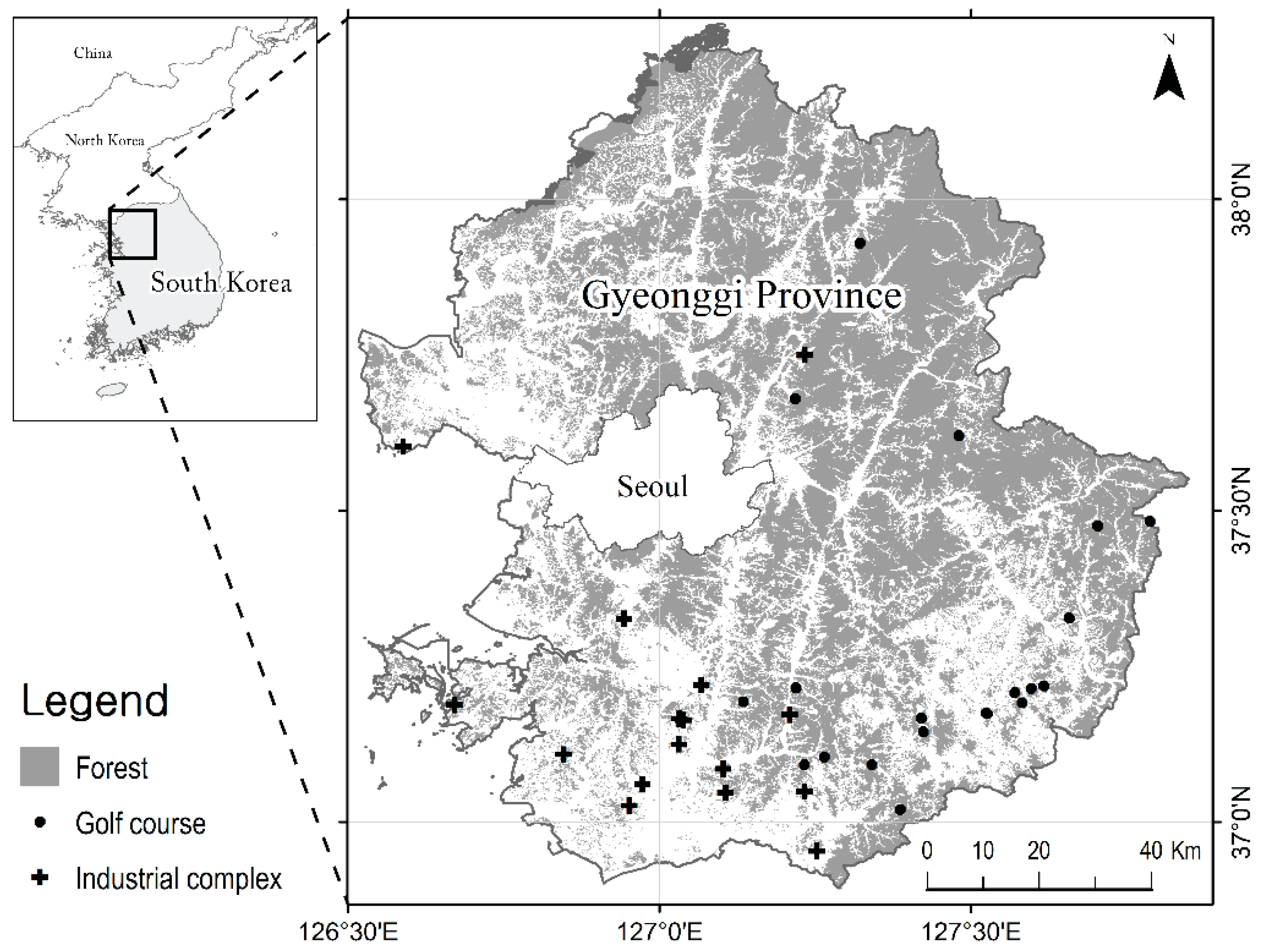
2.1. Study Sites

To collect sample sites, data from Environmental Impact Statements (EISs) between 1982 and 2014 in South Korea were reviewed (about 5000 cases) [26]. A group of developments on forest lands was selected from the EISs according to the following rules, based on previous literature. Development on forest lands was defined in this research as a project that included forest cover greater than 0.1 ha within the project site. Projects having forest cover less than 0.1 ha were excluded to prevent technical errors on spatial analysis using multiple data layers with mutually inconsistent spatial resolutions. Then, for the purpose of statistical analyses, the first and the second largest project types on forest lands were considered study sites. These were “golf course projects” and “industrial complex projects”. To analyze sample sites with similar environmental conditions and levels of development pressure on a regional scale, only sites in the Gyeonggi province were examined in this research (Figure 1).

On a national scale, the industrial complex category accounted for about 20% of existing EIS sites, and sports facility category for about 12%, with golf courses comprising the majority (about 70% of the sports facility category) [26]. Golf courses and industrial complexes were the major types of nationwide development on forest lands during the whole EIA period, and provided a sufficient sample size for this research. In the initial stage, the total number of golf course and industrial complex projects in the Gyeonggi province were 110 and 58, respectively.

Sample sites were defined as the whole development project area upon which a development project is designed. Analysis areas were outside the boundary of the selected sample sites in order to estimate the impact of development on remnant forest in the vicinity of the sample sites, not the sample sites themselves. Through our subjective sampling process, appropriate sample sites were selected based on the following exclusion criteria: (i) forest area at a development site less than 0.1 ha; (ii) sites without updated information on the 1st and 3rd updated land cover maps (LCMs); (iii) development projects on islands; and (iv) linear-shaped developments such as railroads, roads and power lines. By comparing development locations on the two maps using the naked eye, selection of sample sites was undertaken. Considering the land cover changes, 37 study sites were selected: 21 sites for golf courses and 16 sites for industrial complexes.

2.2. Fragmentation Analysis

To investigate land cover changes due to development, fragmentation analysis was introduced, and two national-scale LCMs were used as source data. These maps were provided by South Korea’s Ministry of Environment; one was published in 2007, and the other was updated in 2014. The raster data used in this study have a spatial resolution of 5 m. Three of the 22 categories were related to forest cover: conifer, broadleaf, and mixed forests. While the first LCM was used to select a natural area before development, the second LCM was used to identify the completion of development at project sites. In the initial stage, 17 potential landscape metrics that are frequently used in fragmentation analysis [27,28,29,30,31] were used to accurately detect land cover changes, and a list of the tested metrics is shown in

Table 1. Landscape metrics tested in this study to effectively detect land cover changes caused by development, which were selected after pre- and post-development comparison using analysis of variance (ANOVA). Definitions and formulations of the selected landscape metrics are explained.

	Landscape Metrics
Metrics Selected	- CA, CONNECT, LSI, NP, PD - TE (only for golf courses) or SIMI (only for industrial complexes)
Metrics Excluded	- AREA, CLUMPY, CONTIG, CPLAND, ED, ENN, LPI, NDCA, PLAND, TCA
Definitions (unit)	Formulations
AREA  - Patch Size in Area (ha)	$\mathrm{AREA}=\frac{{{\displaystyle \sum }}_{j=1}^n{X}_{ij}}{n_i}$
CA  - Class Area (ha)	$\mathrm{CA}={\displaystyle \sum _{j=1}^n}{a}_{ij}\left(\frac{1}{10,000}\right)$
CLUMPY  - Clumpiness Index (−)	$\mathrm{CLUMPY}=\left(\frac{G_i-P_i}{P_i}\right)$
CONNECT  - Connectance Index (−)	$\mathrm{CONNECT}=\left[\frac{{{\displaystyle \sum }}_{j=k}^n{\mathrm{e}}_{ijk}}{\frac{n_i\left(n_i-1\right)}{2}}\right]$
CONTIG  - Contiguity Index (−)	$\mathrm{CONTIG}=\frac{\left[\frac{{{\displaystyle \sum }}_{r=1}^z{c}_{ijr}}{a_{ij}}\right]-1}{v-1}$
CPLAND  - Core Area Percentage of Landscape (%)	$\mathrm{CPLAND}=\frac{{{\displaystyle \sum }}_{j=1}^n{a^c}_{ij}}{A}\left(100\right)$
ED  - Edge Density (m/ha)	$\mathrm{ED}=\frac{{{\displaystyle \sum }}_{k=1}^m{e}_{ik}}{A}\left(\frac{1}{10,000}\right)$
ENN  - Euclidean Nearest Neighbor (m)	$\mathrm{ENN}=h_i$
LPI  - Largest Patch Index (%)	$\mathrm{LPI}=\frac{MAX\left(a_{ij}\right)}{A}\left(100\right)$
LSI  - Landscape Shape Index (−)	$\mathrm{LSI}=\frac{e_i}{min{e}_i}$
NDCA  - Number of Disjunct Core Areas (−)	$\mathrm{NDCA}={\displaystyle \sum _{j=1}^n}{a}_{ij}$
NP  - Number of Patches (−)	$\mathrm{NP}=n_i$
PD  - Patch Density (per 100 ha)	$\mathrm{PD}=\frac{n_i}{A}\left(\frac{1}{10,000}\right)\left(\frac{1}{100}\right)$
PLAND  - Percentage of Landscape (%)	$\mathrm{PLAND}=p_i=\frac{{{\displaystyle \sum }}_{j=1}^n{a}_{ij}}{A}\left(100\right)$
SIMI  - Similarity Index (−)	$\mathrm{SIMI}={\displaystyle \sum _{s=1}^n}\frac{a_{ijs}\ast d_{ik}}{h^{2}ijs}$
TCA  - Total Core Area (ha)	$\mathrm{TCA}={\displaystyle \sum _{j=1}^n}{a^c}_{ij}\left(\frac{1}{10,000}\right)$
TE  - Total Edge Length (m)	$\mathrm{TE}={\displaystyle \sum _{k=1}^m}{e}_{ik}$

_i: patch types (from 1 to m); _j: patches (from 1 to m); _k: patch types (from 1 to m); a_ij: area (m²) of patch _ij (or number of cells); G_i: proportion of like adjacency; P_i: proportion of the landscape occupied by patch type _I; C_ijr: contiguity value for pixel _r in patch _ij; v: sum of the value in a 3-by-3 cell template; A: total landscape area (m²); e_ik: total edge length (m) in landscape between patch types _i and _k; h_ij: distance (m) from patch _ij to nearest neighboring patch of the same type (edge-to-edge distance); d_ik: dissimilarity (edge contrast weight) between patch types _i and _k.

.

For the metrics, the following acronyms are used: AREA is used for the mean patch size; CLUMPY for the aggregation of each patch type; CONTIG for the mean contiguity between patches; CPLAND for the percentage of core area in a landscape; ED for Edge Density; ENN for the mean Euclidian distance of the Nearest Neighbors; LPI for Largest Patch Index; PLAND for the Percentage of Landscape; CA for the total Class Area; CONNECT for Connectance Index; LSI for the Landscape Shape Index; NDCA for the Number of Disjunct Core Areas; NP for the Number of Patches; PD for Patch Density; TE for Total Edge length; TCA for Total Core Area; and SIMI for the mean Similarity Index [32]. To examine the impact ranges of forest development, we designed eight concentric buffer zones surrounding individual development sites, from the boundary of a development site to 100, 200, 300, 400, 500, 1000, 1500 and 2000 m away, respectively. Using FRAGSTATS ver. 4.2 [32] (University of Massachussetts, Amherst, MA, USA), the fragmentation values of selected development projects were computed for each buffer zone, and pre- and post-development.

2.3. Statistics

In the EISs, completion dates of projects were not provided, so sample sites were selected based on apparent changes in land use between the two LCMs pre- and post-development. A variety of landscape metrics for pre-development were statistically compared with post-development using repeated measures ANOVA in order to identify which landscape metrics were useful for this analysis. Then, project sites were re-grouped by forest area in order to investigate the effects of size and location on buffer zones. Samples were re-classified and broken down into 30 ha units for within-project-site forest area. The buffer zone effect for the selected landscape metrics was analyzed to examine the development effect based on forest area using repeated measures ANOVA.

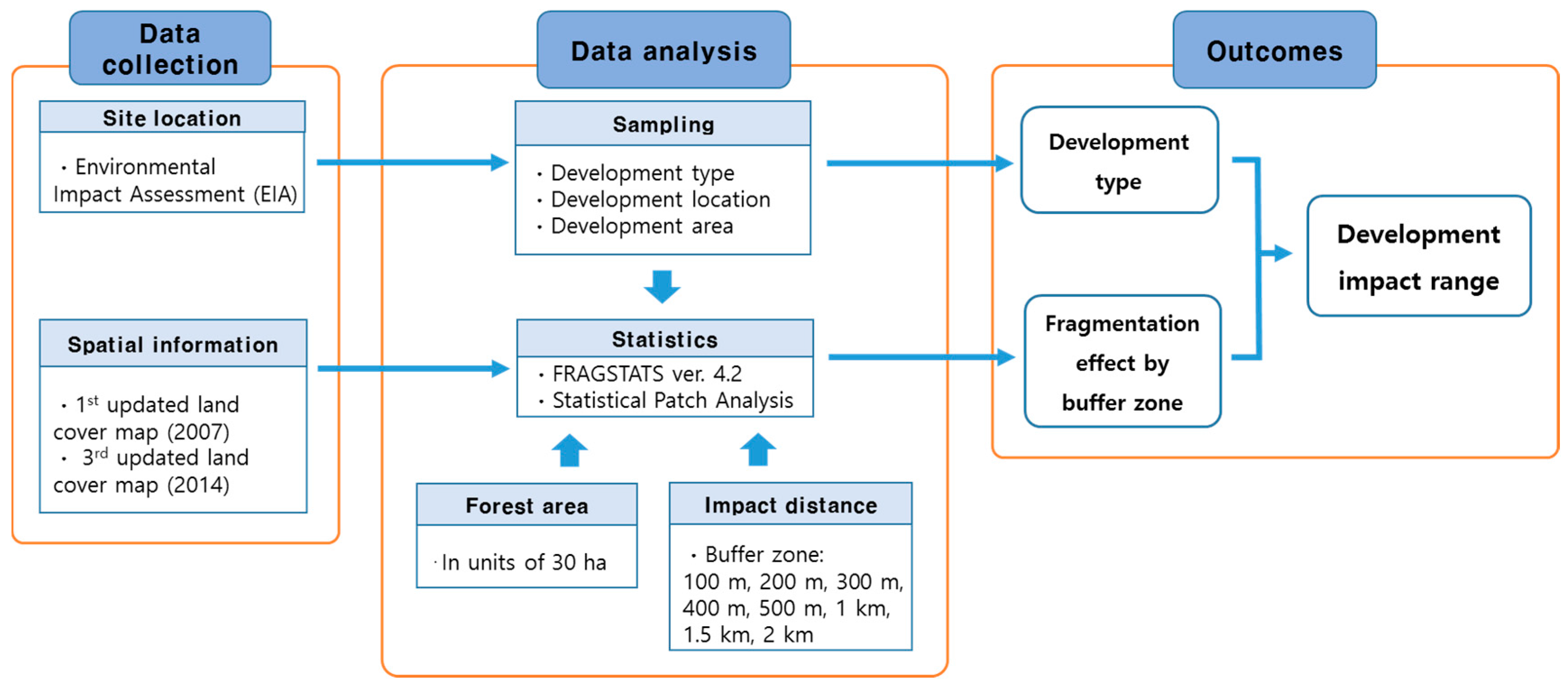
2.4. Analysis Procedure

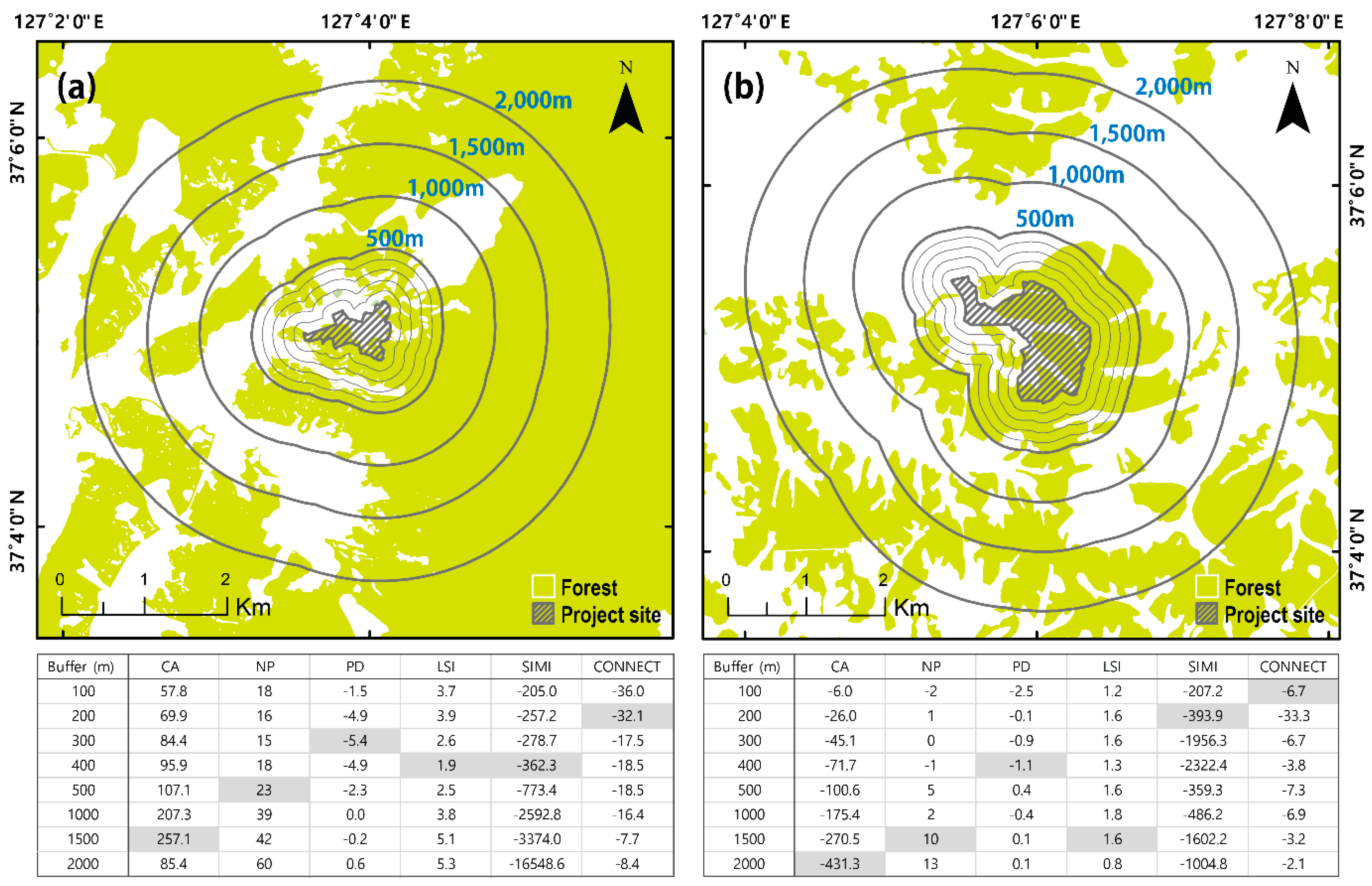
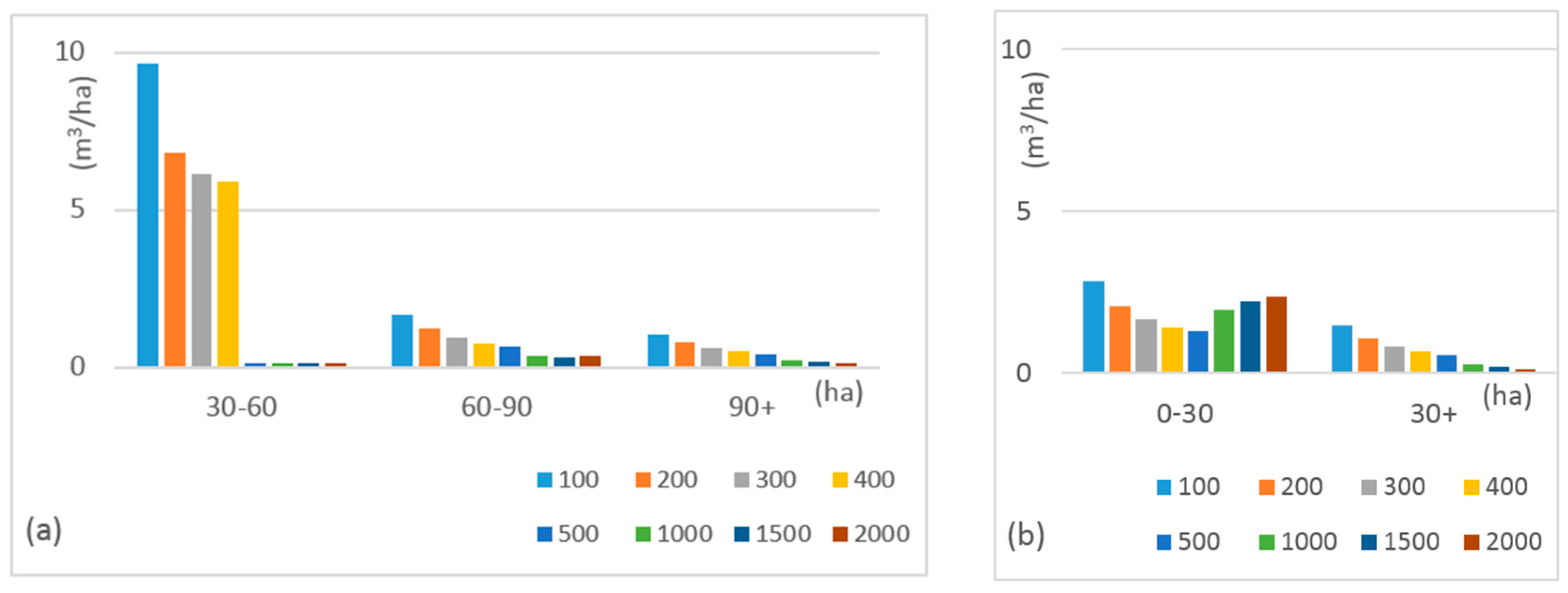
Using the results from fragmentation analysis and repeated measures ANOVA, the impact range for each development, which indicates drastic changes or inconsistent patterns in fragmentation, was investigated in the buffer zone unit. We assumed that a 100 m buffer zone around a project site would be most affected by development, and thus the landscape metrics of the 100 m buffer zone should be compared with those of all the other buffer zones. Because the impact of development on forest is not linear, we explored the differences between buffer zones within the sweep of development impact, which showed consistent fragmentation intensity, and other buffer zones beyond the sweep of development impact, which showed irregular intensity. Based on this concept, we established the impact range for each sample site. The “impact range” was defined in this study as a theoretical distance of equivalent fragmentation impact, regulated by the buffer zone as the unit.

Each metric had a particular distance value indicating the impact ranges, and the results were used to characterize the two development types based on the impact range. As landscape changes over the forested area, including fragmentation, could exert positive or negative effects on the surrounding forest [33,34,35,36,37], the results of this analysis were compared using forestry inventory data in order to examine the ecological effect due to the landscape changes. The overall research process is delineated below in Figure 2.

3. Results

After analysis of land cover changes pre- and post-development for the 17 landscape metrics using repeated measures ANOVA, seven metrics were selected for this research (Table 1) that showed significant changes after the development of golf courses and industrial complexes. The results of repeated measures ANOVA are shown in

Table 2. Analysis of within-subjects effects of all golf courses and industrial complexes with regard to the effects of development and buffer zones for each landscape metric using repeated measures ANOVA.

Golf Course		Type III Sum of Squares	Degree of freedom	Mean Square	F	p-Value
Landscape Metric	Source of Variation
CA	Time	69,435.275	1	69,435.275	2.016	0.158
	Time & buffer	80,134.441	7	11,447.777	0.332	0.938
NP	Time	10,653.762	1	10,653.762	75.248	0.000
	Time & buffer	4743.143	7	677.592	4.786	0.000
PD	Time	44.566	1	44.566	8.316	0.004
	Time & buffer	28.030	7	4.004	0.747	0.632
TE	Time	2.926 × 1010	1	2.926 × 1010	157.822	0.000
	Time & buffer	1.549 × 1010	7	2,213,266,064	11.938	0.000
LSI	Time	469.167	1	469.167	108.217	0.000
	Time & buffer	27.134	7	3.876	0.894	0.513
CONNECT	Time	9033.243	1	9033.243	41.729	0.000
	Time & buffer	4071.675	7	581.668	2.687	0.012
Industrial Complex		Type III Sum of Squares	Degree of freedom	Mean Square	F	p-Value
Landscape Metric	Source of Variation
CA	Time	1,058,086.749	1	1,058,086.749	17.829	0.000
	Time & buffer	466,276.167	7	66,610.881	1.122	0.354
NP	Time	6460.141	1	6460.141	20.904	0.000
	Time & buffer	4654.797	7	664.971	2.152	0.043
PD	Time	528.821	1	528.821	59.177	0.000
	Time & buffer	71.115	7	10.159	1.137	0.345
TE	Time	96.776	1	96.776	13.386	0.000
	Time & buffer	52.607	7	7.515	1.040	0.407
SIMI	Time	353,334,316.7	1	353,334,316.7	13.284	0.000
	Time & buffer	238,791,915.9	7	34,113,130.84	1.282	0.265
CONNECT	Time	1832.154	1	1832.154	5.206	0.024
	Time & buffer	743.772	7	106.253	0.302	0.952

. These results indicate significant differences pre- and post-development in terms of fragmentation impact (p < 0.05).

When samples were re-classified by 30 ha units of forest area, golf courses were separated into three classes—30 to 60 ha, 60 to 90 ha, and over 90 ha, whereas those of industrial complexes were separated into two classes—0 to 30 ha and over 30 ha depending on the overall range of internal forest area of the two project types. The results of buffer zone analysis for golf courses and industrial complexes are shown in Table 2, concentrating on significant landscape metrics including CA, NP, PD, LSI and CONNECT as well as TE for golf courses and SIMI for industrial complexes. The individual effect of all metrics was highly significant except for the CA of golf courses (Table 2). When analyzing the effects of landscape metrics and buffer zones concurrently, however, the effects were, in general, not statistically significant. Thus, there was no consistent significant difference from the 100 m buffer zones to the 2000 m buffer zones. Nevertheless, to identify the fragmentation impacts of the projects, we focused on delimiting a series of buffer zones from the 100 m buffer zone near the epicenter of development to the most distant buffer zone that still showed statistically equivalent fragmentation intensity compared to the rest of the buffer zones. We therefore performed multiple comparison analysis via post hoc testing in repeated measures ANOVA based on forest area for golf courses (

Table 3. Post hoc testing in repeated measures ANOVA analyzing golf course development with a forest area ranging from 30 to >90 ha for six landscape metrics. The values of each buffer zone are compared with those of 100 m buffer zones to identify distinct impact ranges (p < 0.05).

Repeated Measures ANOVA for Golf Courses (Mean Value) 1
Metrics/Buffer Zones	Forest Area (ha)			Metrics/Buffer Zones	Forest Area (ha)
	30~60	60~90	90 +		30~60	60~90	90 +
CA 100 m vs.				TE 100 m vs.
200 m	−25.77	−33.12	−63.21	200 m	−4208.0	−4321.92	−6151.67
300 m	−53.23	−66.50	−124.40	300 m	−9063.0	−8890.77	−10,587.50
400 m	−81.29	−101.04	−184.90	400 m	−13,910.5	−13,704.04	−14,508.33
500 m	−109.43 *	−136.88	−248.56	500 m	−19,201.5	−18,644.35 *	−20,004.17
1000 m	−266.43 *	−367.78 *	−622.87	1000 m	−50,323.0 *	−48,914.42 *	−55,064.17
1500 m	−480.29 *	−697.44 *	−1085.17 *	1500 m	−88,897.5 *	−86,739.23 *	−96,248.33 *
2000 m	−757.57 *	−1105.56 *	−1638.31 *	2000 m	−143,196.5 *	−131,822.69 *	−138,245.83 *
SE2	33.75	61.71	236.24	SE	8970.79	5099.21	20,851.76
NP 100 m vs.				LSI 100 m vs.
200 m	−0.8	−0.23	−1.67	200 m	−0.42	−0.30	0.03
300 m	−2.9	−1.96	−0.33	300 m	−0.94	−0.70	0.15
400 m	−5.4	−4.23	−2.50	400 m	−1.40	−1.16	0.21
500 m	−6.6	−5.04	−8.67	500 m	−1.85	−1.54	−0.10
1000 m	−19.9	−14.39 *	−17.17	1000 m	−4.59 *	−3.76 *	−1.67
1500 m	−34.6 *	−23.62 *	−23.00	1500 m	−7.00 *	−5.59 *	−3.18
2000 m	−56.2 *	−37.58 *	−38.17	2000 m	−9.86 *	−7.42 *	−5.45
SE	6.20	3.93	13.56	SE	1.25	0.77	2.28
PD 100 m vs.				CONNECT 100 m vs.
200 m	2.51	2.72 *	0.64	200 m	6.48	−2.01	3.10
300 m	2.83	3.12 *	1.60	300 m	−1.10	7.29	7.62
400 m	2.77	3.22 *	1.58	400 m	6.49	12.58	12.30
500 m	3.56	3.66 *	1.02	500 m	11.35	12.95	15.34
1000 m	4.21 *	4.16 *	1.64	1000 m	22.35 *	27.16 *	18.40
1500 m	4.66 *	4.54 *	2.19	1500 m	25.44 *	27.31 *	16.14
2000 m	4.71 *	4.63 *	1.41	2000 m	26.85 *	32.10 *	20.11
SE	1.28	0.84	0.80	SE	5.99	6.13	8.42

Tukey HSD test (p = 0.05); ¹ ‘100 m buffer zone’ minus ‘other buffer zones’; * Significant at p-values less than 0.05.

) and industrial complexes (

Table 4. Post hoc testing in repeated measures ANOVA analyzing industrial complex projects with forest areas ranging from 0 to > 30 ha for six landscape metrics. The values of each buffer zone are compared with those of 100 m buffer zones to identify distinct impact ranges (p < 0.05).

Repeated Measures ANOVA for Industrial Complexes (Mean Value) 1
Indexes/Buffer Zones	Forest Area (ha)		Indexes/Buffer Zones	Forest Area (ha)
	0~30	30 +		0~30	30 +
CA 100 m vs.			LSI 100 m vs.
200 m	−18.50	−15.20	200 m	−0.35	−0.32
300 m	−37.86	−29.26	300 m	−0.81	−0.63
400 m	−59.03	−44.70	400 m	−1.24	−1.12
500 m	−82.06	−62.26	500 m	−1.76 *	−1.54
1000 m	−218.12	−192.13 *	1000 m	−4.25 *	−3.22 *
1500 m	−400.04 *	−368.13 *	1500 m	−6.55 *	−5.43 *
2000 m	−629.77 *	−588.48 *	2000 m	−8.59 *	−7.27 *
SE2	74.86	44.31	SE	0.54	0.51
NP 100 m vs.			SIMI 100 m vs.
200 m	−0.92	0.00	200 m	−279.51	−43.82
300 m	−2.92	−3.33	300 m	−596.85	−299.51
400 m	−5.04	−5.83	E	−574.15	−371.26
500 m	−6.19	−6.67	500 m	E	−56.10
E	−18.04 *	−16.83	1000 m	−1505.12	−254.72
1500 m	−32.08 *	−30.00	1500 m	−319.40	−622.45
2000 m	−48.89 *	−46.33 *	2000 m	−5651.88 *	−715.27
SE	3.49	11.11	SE	1515.28	338.71
PD 100 m vs.			CONNECT 100 m vs.
200 m	4.73 *	3.72	200 m	8.66	−2.98
300 m	5.61 *	3.98	300 m	15.07 *	9.21
400 m	5.96 *	4.20	400 m	18.81 *	10.75
500 m	6.78 *	5.00	500 m	19.82 *	12.07
1000 m	7.44 *	5.68 *	1000 m	31.03 *	15.65
1500 m	7.78 *	5.74 *	1500 m	33.03 *	17.75
2000 m	8.00 *	5.82 *	2000 m	35.11 *	19.00
SE	1.09	1.53	SE	4.30	10.11

Tukey HSD test (p = 0.05); ¹ ‘100 m buffer zone’ minus ‘other buffer zones’; * Significant at p-values less than 0.05.

).

Based upon our assumption that a 100 m buffer zone is the most affected by development, the 100 m buffer zones of each project site were compared with all other buffer zones by each landscape metric. In the case of golf courses with forest areas less than 60 ha (Table 3), the CA values of 100 m buffer zones were significantly different than buffer zones equal to or greater than 500 m. Consequently, eight buffer zones were separated into two groups with regard to CA values (p < 0.05): 100 to 400 m buffer zones and 500 to 2000 m buffer zones (Table 3). This outcome implied that the entire region within 400 m of the development site faced the same fragmentation impact intensity, while beyond that range the impact intensity varied. This result with regard to CA varied among the forest area classes; at 60 to 90 ha, the 500 m buffer zones showed uniform CA, while sites over 90 ha had expanded impact ranges up to 2000 m away. This pattern was diverse for the landscape metrics analyzed in this research (Table 3).

For industrial complexes with forest areas less than 30 ha (Table 4), the CONNECT values of 100 m buffer zones varied from those of 300 m buffer zones. Therefore, 100 to 200 m buffer zones were distinguished from 300 to 2000 m buffer zones (p < 0.05; Table 4). Using this approach, the results from multiple fragmentation analysis for both project types are presented in

Table 5. Impact ranges in meters for each landscape metric by forest area for golf courses and industrial complexes.

Golf Courses	Forest Area (ha)	Landscape Metrics (m)
		CA	NP	PD	TE	LSI	CONNECT	Mean	Mean * (Representative)
	30~60	500	1000	500	500	500	500	580	670
	60~90	500	500	100	400	500	500	420	330
	Over 90	1000	2000	2000	1000	2000	2000	1670	1670
Industrial Complexes	Forest Area (ha)	Landscape Metrics (m)
		CA	NP	PD	LSI	SIMI	CONNECT	Mean	Mean * (Representative)
	0~30	1000	500	100	400	1500	200	620	270
	Over 30	500	1500	500	500	2000	2000	1170	1330
Definitions							Major Landscape Metric Elements
CA:  NP:  PD:  TE:  LSI:  SIMI:  CONNECT			class area no. of patches patch density total edge length landscape shape index similarity index connectance index				➔ patch area ➔ no. of patches ➔ no. of patches ➔ edge length ➔ edge length ➔ patch area, distance between patches ➔ joining conditions of a certain patch type (joined or unjoined)

* The average value of the shaded landscape metrics indicating similarity between the impact ranges and the mean values computed from all landscape metrics.

.

In Table 5, samples with forest areas over 90 ha seemed to affect surrounding landscapes most among the three groups. The main pattern of the impact range based on forest area was calculated from the average values of the six selected metircs values for each forest area group, i.e., 580 m for the 30 to 60 ha forest area group, 420 m for the 60 to 90 ha group and 1670 m for the over 90 ha group (Table 5). Three metrics, NP, PD and TE, were most representative of the main pattern. For example, in the case of NP, while sites with 30 to 60 ha of forest area showed an impact range of 1000 m, sites of over 90 ha had a 2000 m impact range. Sites of 60 to 90 ha had the smallest impact range of 500 m, and this phenomenon was similar to the main pattern shown in Table 5. The fundamental attributes characterizing golf courses were summarized as the number of patches derived from NP and PD and the edge length from TE according to the major elements of the representative landscape metrics (Table 5) [32]. In industrial complex analysis, the larger forest area group showed a greater impact, with average values of 620 m for forest areas of 0 to 30 ha and 1170 m for those over 30 ha (Table 5). Three metrics, NP, PD and CONNECT, had a dominant role in determining the main pattern of the impact range (Table 5). CONNECT varied from the values found for golf course analysis, as described above. These three metrics were derived primarily from the number of patches (NP, PD) and the joining conditions of a certain patch type (CONNECT) (Table 5) [32]. In conclusion, this result revealed that while the “edge length” of TE represented the unique characteristic of golf courses, the “joining conditions of patches” of CONNECT was considered as an useful delegate element for industrial complexes (Table 5).

Comparing golf courses with industrial complexes, there was a difference in the most representative landscape metrics of the main patterns shaded in Table 5. While NP and PD were selected for both types, TE was only applicable to golf courses and CONNECT was only applicable to industrial complexes. Because NP and PD were considered the most representative metrics for both development types; however, they were not useful for effectively differentiating between the two development types in terms of landscape change after development. Instead, TE, which originated from the edge length, and CONNECT, which is determined based on configuration by patch type, were considered valuable metrics for distinguishing golf courses from industrial complexes in terms of fragmentation impact.

According to the results from TE (Table 5), golf courses disturbed the forest areas surrounding developments more than industrial complexes. From this, it can be deduced that golf courses triggered additional development, which inevitably affected the edge region. The CONNECT of industrial complexes indicated that this type of development interrupted the aggregation of congeneric patches and/or divided the patches. This implied that industrial complexes might cause more serious changes in adjacent areas on a patch scale, such as damage due to secondary development, than golf course development. Additionally, golf courses with the minimum forest area showed a greater impact range than the medium-sized group, which was an unexpected result in this research (Table 5). In contrast, the impact ranges of industrial complexes increased with the size of forest areas within project sites. Based upon the results explained above, we compared the application of our approach with the actual development of two industrial complexes in Figure 3 ((a) 0 to 30 ha; (b) over 30 ha).

While relatively narrower impact ranges with an average of 550 m were discovered in the case of the smaller project (Figure 3a), in the larger project (Figure 3b), wider ranges with an average of 814 m were identified. These results were mostly consistent with the major findings in this research (Table 5); however, there was an issue concerning the interpretation of the impact range of individual developments. As the impact range values were closely related to the proportion of forest and developed areas around the project sites and their configuration, a comprehensive understanding of the historical background of landscape changes in a target area is needed to estimate such ranges properly. To examine the relationship between the results from our impact range analyses and ecological factors, stem volume growth data from the national vegetation survey of the Korea Forest Service were analyzed. The tree species growth per hectare was computed using datasets from two different selected time periods, 2008 and 2013, and the results in relation to the two project types are presented in Figure 4.

As the sample size was limited due to the resolution of the dataset, statistical analysis of the effects of buffer zones in relation to forest area was not available. In Figure 4, the smallest golf course group of 30 to 60 ha showed the highest growth rate for the same period compared to other larger forest area groups. The smaller forest area group of industrial complexes had a relatively higher growth rate than the larger forest area group, but not to the same extent as golf courses (Figure 4). For both golf courses and industrial complexes, the growth rates in the 100 m buffer zone, regardless of the forest area, were highest (golf courses by forest area: 9.6, 1.7, 1.1 m³/ha/5 years; industrial complexes by forest area: 2.8, 1.5 m³/ha/5 years; Figure 4). This tendency for the growth rates to decrease with greater distance from the project site might be due to the management of development boundaries for the purpose of minimizing environmental impacts. However, further accurate and detailed analysis is needed that is beyond the scope of this study.

4. Discussion

In this study, an approach to quantifying the impacts of development was created based upon landscape change analysis and the buffer zone concept. Differences in metrics between golf courses and industrial complexes emerged from the analysis of several landscape metrics based on forest area within project sites. There was a difference between the two development types in terms of the major landscape changes on the following landscape metrics: NP, PD and TE for golf courses; and NP, PD and CONNECT for industrial complexes. Whereas the impact range of golf courses was not related to forest area in the project site, which of industrial complexes increased with remnant forest size. Consequently, the results of this research indicate that different types of development have varying effect patterns on forest areas. When we tested this outcome with individual projects, each sample bore similarities to the pattern suggested for that development type by our analysis, though there was some individual variation. Therefore, the findings here provide a meaningful basis for creating a useful tool in order to quantify development impacts in a simple and visible manner.

The novel approach in this research can be applied to modeling and assessing environmental impacts in various regions and countries. There has been little research on an international scale that systematically deals with the fragmentation impacts of development projects listed in EIAs, for example, urban development [7,8,27] and golf course development [38,39,40]. As there are significant differences among EIA categories due to the innate attributes of each project type, standardized criteria for evaluating development projects are needed that will also consider multiple categories, especially in relation to forest areas. In this sense, it is essential that future studies cover various development types and create a comprehensive assessment model based on accumulated comparative research.

There are two limitations to this research that should be considered in order to improve the degree of accuracy and reliability of this analysis. First, to better understand the implications of this analysis, a comparison of the changes in landscape patterns and the ecological structure and functions in areas without a history of previous development is needed. From this comparison, the reason for landscape changes and the intensity of impacts could be clarified. The most challenging part of this task is to find comparable sites that share similar characteristics except for the existence of development. Secondly, buffer zone analysis needs to be compared with an equal sized sampling method such as a transect sampling. We tested our buffer zone concept here, in order to minimize the effects of external factors on the fragmentation pattern, which is beyond the scope of this study. In order to obtain more reliable output, the issues of spatial scaling [41] and compatibility with ecological theory [42] should be addressed in the sampling design stage. Follow-up research exploring these points would contribute to the assessment of landscape changes under diverse situations.

References

1. Korea Forest Service. Available online: http://www.forest.go.kr (accessed on 12 August 2015).
2. Nilon, C.H.; Long, C.N.; Zipperer, W.C. Effects of wildland development on forest bird communities. Landsc. Urban Plan. 1995, 32, 81–92. [Google Scholar] [CrossRef]
3. Young, A.; Boyle, T.; Brown, T. The population genetic consequences of habitat fragmentation for plants. Trends Ecol. Evol. 1996, 11, 413–418. [Google Scholar] [CrossRef]
4. Theobald, D.M.; Miller, J.R.; Hobbs, N.T. Estimation the cumulative effects of development on wildlife habitat. Landsc. Urban Plan. 1997, 39, 25–36. [Google Scholar] [CrossRef]
5. Mckinney, M.L. Urbanization, biodiversity, and conservation. Bioscience 2002, 52, 883–890. [Google Scholar] [CrossRef]
6. Marzluff, J.M.; Ewing, K. Restoration of fragmented landscapes for the conservation of birds: A general framework and specific recommendations for urbanizing landscapes. Restor. Ecol. 2001, 9, 280–292. [Google Scholar] [CrossRef]
7. Hansen, A.J.; Knight, R.L.; Marzluff, J.M. Effects of exurban development on biodiversity. Ecol. Appl. 2005, 15, 1893–1905. [Google Scholar] [CrossRef]
8. Munroe, D.K.; Croissant, C.; York, A.M. Land use policy and landscape fragmentation in an urbanizing region: Assessing the impact of zoning. Appl. Geogr. 2005, 25, 121–141. [Google Scholar] [CrossRef]
9. Borgmann, K.B.; Rodewald, A.D. Forest restoration in urbanizing landscapes: Interactions between land uses and exotic shrubs. Restor. Ecol. 2005, 13, 334–340. [Google Scholar] [CrossRef]
10. Gonzalez-Abraham, C.E.; Radeloff, V.C.; Hammer, R.B. Building patterns and landscape fragmentation in northern Wisconsin, USA. Landsc. Ecol. 2007, 22, 217–230. [Google Scholar] [CrossRef]
11. Cho, K.J.; Ro, T.H. Environmental Impact Assessment system. Korea Environ. Policy Bull. 2012, 10, 1–19. [Google Scholar]
12. Lee, J.Y.; Lee, J.H. Actual factors influencing EIA system’s validity. J. Environ. Policy Adm. 1999, 7, 19–46. [Google Scholar]
13. Choi, H.S. A study on the improvements for the legal systems related to the conservation of mountain ridge areas—In case of Whasung. J. Korean Soc. Environ. Restor. Technol. 2009, 12, 133–144. [Google Scholar]
14. Jung, B.G. A note on the problems and alternative improvement of environmental impact Assessment in Korea—Evaluation in an engineer’s viewpoint. Public Law J. 2009, 10, 327–349. [Google Scholar]
15. No, H.W.; Choi, H.S. The improvements for the altitude criteria related to the adaptive reuse permission on mountains district—With special emphasis on ‘Management of Mountains District Act’ and ‘National Land Planning and Utilization Act’. J. Korean Soc. Rural Plan. 2011, 17, 81–90. [Google Scholar] [CrossRef]
16. Gehlhausen, S.M.; Schwartz, M.W.; Augspurger, C.K. Vegetation and microclimatic edge effects in two mixed-mesophytic forest fragments. Plant Ecol. 2000, 147, 21–35. [Google Scholar] [CrossRef]
17. Kupfer, J.A.; Runkle, J.R. Edge-mediated effects on stand dynamic processes in forest interiors: A coupled field and simulation approach. Oikos 2003, 101, 135–146. [Google Scholar] [CrossRef]
18. Harper, K.A.; Macdonald, E.; Burton, P.J. Edge influence on forest structure and composition in fragmented landscapes. Conserv. Biol. 2005, 19, 768–782. [Google Scholar] [CrossRef]
19. McDonald, R.I.; Urban, D.L. Edge effects on species composition and exotic species abundance in the North Carolina Piedmont. Biol. Invasions 2006, 8, 1049–1060. [Google Scholar] [CrossRef]
20. Ewers, R.M.; Didham, R.K. The effect of fragment shape and species’ sensitivity to habitat edges on animal population size. Conserv. Biol. 2007, 21, 926–936. [Google Scholar] [CrossRef] [PubMed]
21. Chas-Amil, M.L.; Touza, J.; García-Martínez, E. Forest fires in the wildland-urban interface: A spatial analysis of forest fragmentation and human impacts. Appl. Geogr. 2013, 43, 127–137. [Google Scholar] [CrossRef]
22. Herzog, F.; Lausch, A.; Müller, E.; Thulke, H.; Steinhardt, U.; Lehmann, S. Landscape metrics for assessment of landscape destruction and rehabilitation. Environ. Manag. 2001, 27, 91–107. [Google Scholar] [CrossRef] [PubMed]
23. Mörtberg, U.M.; Balfors, B.; Knol, W.C. Landscape ecological assessment: A tool for integrating biodiversity issues in strategic environmental assessment and planning. J. Environ. Manag. 2007, 82, 457–470. [Google Scholar] [CrossRef] [PubMed]
24. Sitzia, T.; Campagnaro, T.; Grigolato, S. Ecological risk and accessibility analysis to assess the impact of roads under Habitats Directive. J. Environ. Plan. Manag. 2016. [Google Scholar] [CrossRef]
25. Trentanovi, G.; Lippe, M.; Sitzia, T.; Ziechmann, U.; Kowarik, I.; Cierjacks, A. Biotic homogenization at the community scale: Disentangling the roles of urbanization and plant invasion. Divers. Distrib. 2013, 19, 738–748. [Google Scholar] [CrossRef]
26. Environmental Impact Assessment Support System. Available online: https://eiass.go.kr (accessed on 12 October 2015).
27. Swenson, J.J.; Franklin, J. The effects of future urban development on habitat fragmentation in the Santa Monica Mountains. Landsc. Ecol. 2000, 15, 713–730. [Google Scholar] [CrossRef]
28. Stenhouse, R.N. Fragmentation and internal disturbance of native vegetation reserves in the Perth metropolitan area, Western Australia. Landsc. Urban Plan. 2004, 68, 389–401. [Google Scholar] [CrossRef]
29. Zeng, H.; Wu, X.B. Utilities of edge-based metrics for studying landscape fragmentation. Comput. Environ. Urban 2005, 29, 159–178. [Google Scholar] [CrossRef]
30. Yu, X.; Ng, C. An integrated evaluation of landscape change using remote sensing and landscape metrics: A case study of Panyu, Guangzhou. Int. J. Remote Sens. 2006, 27, 1075–1092. [Google Scholar] [CrossRef]
31. Baskent, E.Z.; Kadioğullari, A.I. Spatial and temporal dynamics of land use pattern in Turkey: A case study in İnegöl. Landsc. Urban Plan. 2007, 81, 316–327. [Google Scholar] [CrossRef]
32. McGarigal, K.; Marks, B.J. FRAGSTATS Ver. 4: Spatial Pattern Analysis Program for Quantifying Landscape Structure; General Technical Report; U.S. Department of Agriculture, Forest Service, Pacific Northwest Research Station: Portland, OR, USA, 1995.
33. Bohn, F.J.; Frank, K.; Huth, A. Of climate and its resulting tree growth: Simulating the productivity of temperate forests. Ecol. Model. 2014, 278, 9–17. [Google Scholar] [CrossRef]
34. Bregman, T.P.; Sekercioglu, C.H.; Tobias, J.A. Global patterns and predictors of bird species responses to forest fragmentation: Implications for ecosystem function and conservation. Biol. Conserv. 2014, 169, 372–383. [Google Scholar] [CrossRef]
35. Faaborg, J.; Brittingham, M.; Donovan, T.; Blake, J. Habitat Fragmentation in the Temperate Zone: A Perspective for Managers. In Ecology and Management of Neotropical Migratory Birds: A Synthesis and Reviews of Critical Issues; Martin, T.E., Finch, D.M., Eds.; Oxford University Press: New York, NY, USA, 1995; pp. 331–338. [Google Scholar]
36. Spiecker, H. Silvicultural management in maintaining biodiversity and resistance of forest in Europe-temperate zone. J. Environ. Manag. 2003, 67, 55–65. [Google Scholar] [CrossRef]
37. Ziter, C.; Bennett, E.M.; Gonzalez, A. Temperate forest fragments maintain aboveground carbon stocks out to the forest edge despite changes in community composition. Oecologia 2014, 176, 893–902. [Google Scholar] [CrossRef] [PubMed]
38. Colding, J.; Folke, C. The role of golf courses in biodiversity conservation and ecosystem management. Ecosystems 2009, 12, 191–206. [Google Scholar] [CrossRef]
39. Porter, E.E.; Forschner, B.R.; Blair, R.B. Woody vegetation and canopy fragmentation along a forest-to-urban gradient. Urban Ecosyst. 2001, 5, 131–151. [Google Scholar] [CrossRef]
40. Saarikivi, J.; Knopp, T.; Granroth, A. The role of golf courses in maintaining genetic connectivity between common frog (Rana temporaria) populations in an urban setting. Conserv. Genet. 2013, 14, 1057–1064. [Google Scholar] [CrossRef]
41. Dungan, J.L.; Perry, J.N.; Dale, M.R.T.; Legendre, P.; Citron-Pousty, S.; Fortin, M.-J.; Jakomulska, A.; Miriti, M.; Rosenberg, M.S. A balanced view of scale in spatial statistical analysis. Ecography 2002, 25, 626–640. [Google Scholar] [CrossRef]
42. Gustafson, E.J. Quantifying landscape spatial pattern: What is the state of the art? Ecosystems 1998, 1, 143–156. [Google Scholar] [CrossRef]
Figure 1. Locations of golf course and industrial complex development sites within Gyeonggi Province, Republic of Korea.
Sustainability 08 01012 g001
Figure 2. Procedure for fragmentation analysis of forest land development using FRAGSTATS ver. 4.2 (University of Massachussetts, Amherst, MA, USA) to analyze source data from two land cover maps (from different time periods) and eight different buffer zones.
Sustainability 08 01012 g002
Figure 3. Examples of the development of industrial complexes: (a) 1 to 30 ha of forest area within the project site; and (b) over 30 ha of forest area. Impact ranges for each landscape metric are shaded.
Sustainability 08 01012 g003
Figure 4. Relative stem volume growth for each buffer zone by forest area between 2008 and 2013: (a) golf courses; and (b) industrial complexes.
Sustainability 08 01012 g004