Stochastic Forecast of the Financial Sustainability of Basic Pension in China

Abstract

The paper focuses on the stochastic forecast of the financial sustainability ofbasic pension, based on predictions for the population of China. The population was calculated iteratively by using Leslie matrix. An auto-regressive moving average model was adapted for the predictions of the fertility rates and the mortality rates. The Monte Carlo stochastic method was adapted for the projections of the dynamic process of the financial sustainability of the basic pension from 2013 to 2087 by 5000 times simulation. The forecasting results show that the imbalance of basic pension will occur in 2026. If the statutory retirement age is postponed by five years, the occurrence of the financial gap of the basic pension may be delayedby about 20 years, and the median deficit of basic pension will be reduced by about 64.25% in 2087.

1. Introduction

A basic pension system is one of the most important parts of a social security system. The sustainable development of it has a close relationship with social harmony as well as economic sustainable development [1]. Therefore, it is essential to keep the long-term balance of contributions and expenditures of a basic pension in order to accomplish sustainable development of the system [2,3,4]. In other words, financial sustainability should be maintained.

A basic pension system represents the most essential social protection for the elderly [5]. At present, many developed countries have already entered an aging society, and many developing countries are or will be on the way to it. With the acceleration of the aging evolution of the population, a basic pension fund is confronted with serious payments crisis and financial crisis, severe challenges to sustainable development. The aging of the population has a serious impact on the sustainable development of a basic pension system [6,7,8,9,10]. Therefore, the sustainability of basic pension systems is becoming a hotly discussed issue across the world. There have been many studies that are in attempts to quantify the contributions and expenditures of the pension systems that result from populations aging [11,12,13,14]. These studies mainly introduced two approaches to forecasting the financial sustainability of a basic pension system: the deterministic forecasting method and the stochastic forecasting method. In the deterministic forecasting method, a series of values are preset as the input variables, and the point-estimated value may be obtained as the output result. In the stochastic forecasting method, the stochastic volatility with time is introduced into the input variables, so it may reveal ideal interval estimation and probability distribution under a certain probability. Therefore, the stochastic forecasting method is much better at assessing the future uncertainty of the contributions and expenditures of pension insurance, evaluating the sustainable development of pension insurance system, and controlling the risk topension funds.

China was one of the first among developing countries to have an aging society, and now has the largest old-age population in the world [15]. In recent decades, population aging in China has progressed rapidly, which contributes to the dramatic increase of the dependency ratio of the basic pension system in the future [16]. The expenditure on a basic pension, which mainly depends on the size of the older population, will face unprecedented payment pressure [17], so the financial sustainability of the basic pension will be vulnerable. This has aroused extensive attention as well as heated discussion among all social circles. In recent years, a lot of native scholars and experts have researched the financial sustainability of China’s basic pension from different perspectives by applying various methods [18,19,20,21,22,23,24,25]. Studies have attempted to forecast the financial sustainability of the pension systems mainly by using the deterministic forecasting method; few studies adopted the stochastic forecasting method.

According to the type of population, China’s current pension system is mainly divided into four parts: a basic pension system for urban employees, an old-age insurance system in government bodies and institutions, an endowment insurance system for urban residents, and a new type of social pension system for rural areas. China’s basic pension system for urban employees was undertaken in 1997 and subsequently has had refinements and become relatively mature. It adopts acombination of the social pool account and the individual account. The social pool account is the unfunded pay-as-you-go (PAYG) system where current workers financially support current pensioners, and the individual account is the funding system. The old-age insurance system in government bodies and institutions is a retirement system through fiscal financing. The endowment insurance system for urban residents and the new type of social pension system for rural areas began, respectively, with a pilot implementation in 2009 and 2011, and developed relatively late. As the biggest obstacle to future pension payment mainly stems from the social pool fund (i.e., basic pension), this paper, therefore, focuses on the stochastic forecast of the financial sustainability of the basic pension.

This paper is composed of six sections. The first section raises research questions. The second section mainly constructs astochastic forecasting model for the financial sustainability of the basic pension and assumes data. The third section defines and estimates parameters. The population and wages parameters in the model are considered as random variables, and the time- series estimation method and Leslie Matrix method are used to project the parameters. The fourth section forecasts and analyzes the results. The Monte Carlo stochastic method is used to forecast the financial sustainability of the basic pension. The following section stochastically simulates the financial status of the basic pension on the assumption of postponing retirement by five years. The final section presents conclusions.

2. Forecasting Models and Data Assumptions

2.1. Forecasting Models

According to the current financial incomes and expenses of the basic pension fund for Chinese urban employees, the contributions of the basic pension are mainly paid by enterprises as a certain proportion of their total amount of taxable salaries. The annuities of retired workers are calculated by multiplying the average wages of staff and workers at post over the previous year by the corresponding coefficient. For a given year, once the values of contributions and annuities have been determined, the amount of end-of-year balances is identified by starting with beginning-of-year balances, adding annual contributions, and subtracting annual expenditures. Therefore, the stochastic actuarial forecasting models for the long-term financial status of the basic pension are established as follows.

The contributions of the basic pension are:

$$C_t=C{R}_t\times W_t\times P_{t,a},$$

(1)

where

$C_t$—Contributions of the basic pension in year t;

$C{R}_t$—Contribution rate of the basic pension in year t;

$W_t$—Average wages of employed person in year t;

$P_{t,a}$—Population of insured employees in year t.

The expenditures of the basic pension are:

$$E_t=R{R}_t\times W_t\times P_{t,b},$$

(2)

where

$E_t$—Expenditures of the basic pension in year t;

$R{R}_t$—Replacement rate of the basic pension in year t;

$P_{t,b}$—Population of retired employees in year t.

The accumulated balances of the basic pension are:

$$T_t=(C_t-E_t)+T_{t-1}\times (1+r_t),$$

(3)

where

$T_t$—Accumulated balances of the basic pension in year t;

$T_{t-1}$—Accumulated balances of the basic pension in year t−1;

$r_t$—Return rate of the basic pension fund in year t.

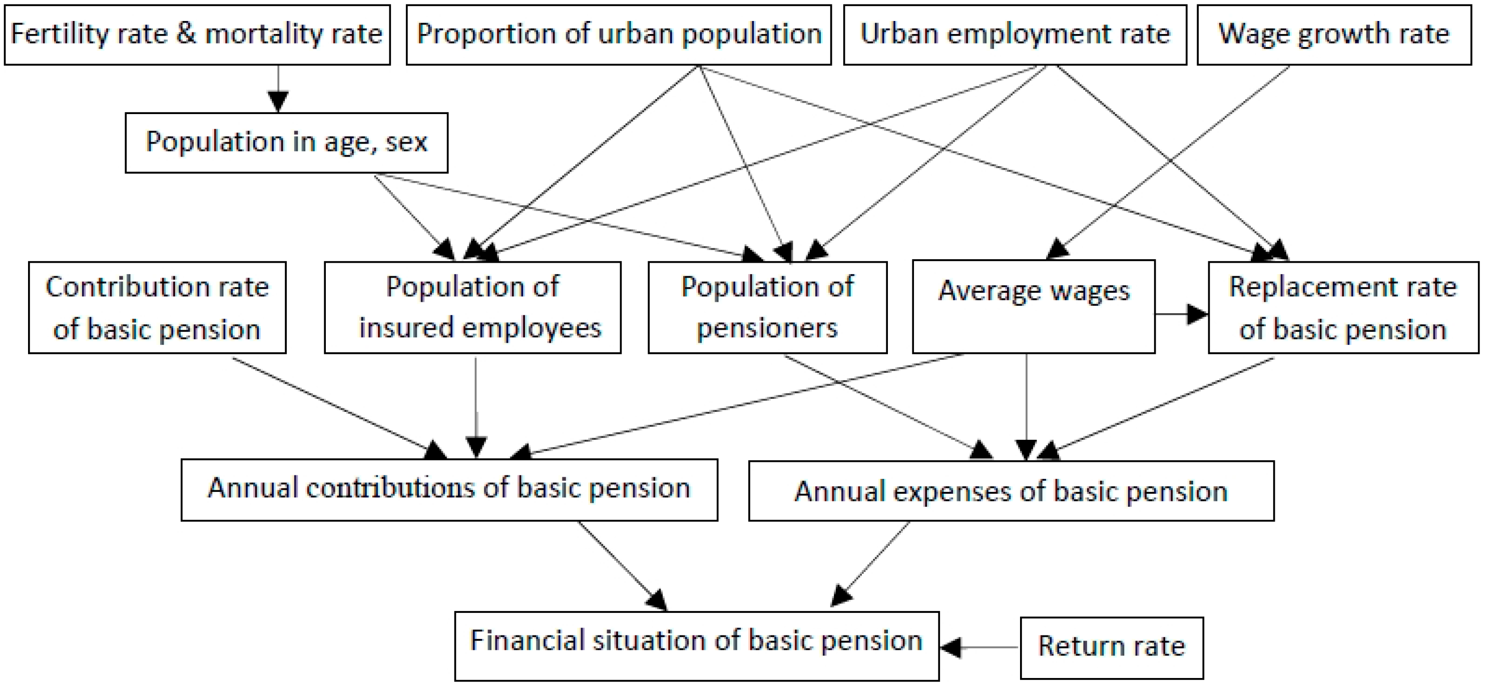
The above models show that the financial situation of the basic pension mainly depends on the number of insured employees and pensioners, average wage for workers, as well as contribution rate, replacement rate, and return rate of the basic pension. Among them, the number of insured employees and pensioners mainly depends on the fertility rate, mortality rate, urban employment rate, and the proportion of the urban population. The average wage of an employed person mainly depends on the wage growth rate. Figure 1 shows the influence path of the above variables on the future financial situation of the basic pension.

Figure 1. Influence path of variables on the future financial situation of the basic pension.

Figure 1. Influence path of variables on the future financial situation of the basic pension.

2.2. Data Assumption

• Initial population data. This paper takes the population data from 2013 as the initial population data.
• Working age. According to the data from China Population & Employment Statistics Yearbook 2014, the educational status of urban employed persons in 2013 was as follows: the proportion of unschooled persons was 0.9%, primary school 9.5%, junior secondary school 39.0%, senior secondary school 24.1%, college 15.0%, university 10.4%, and graduate and higher level 1.0%. Suppose that the urban residents get their jobs when they are 16 years old after receiving primary school education, 17 years old after junior secondary school education, 19 years old after senior secondary school education, 21 years old after college education, 23 years old after university education, and 28 years old after postgraduate and above education. Then, the average working age is calculated from the weighted average of the educational attainment of urban employed persons, and the average working age is about 18.65. Therefore, we suppose that the working age is 19 and everyone may live up to age 100.
• Retirement age. At present, the retirement age in China is 60 for men, 55 for female civil servants, and 50 for female workers. Suppose that the retirement age is 60 for men and 55 for women.
• Percent male births. According to the data from the national statistics bureau, the sex ratio at birth has decreased from 120.56 in 2008 to 115.88 in 2014, or in other words, a decline in the proportion of male births from 54.66% to 53.68%. Keeping the sex ratio at birth in the normal range is one of the key factors for a harmonious society and the normal range declared by the United Nations is 102–107. Therefore, we assume that the sex ratioat birth is 112 during the forecast period, meaning that the percentage of male births is 52.83%.
• Contribution rate. In 2005, the State Council issued a regulation on the establishment of a unified basic old-age insurance system for enterprise employees. According to the regulation, enterprises pay 20% of the sum of taxable salary to form the social pool funds as a basic pension. Then we suppose that the contribution rate of the basic pension is still 20%.
• Coverage rate. The coverage of a basic pension insurance system for urban employees has expanded year by year, increasing from 30.5% in 1990 to 63.23% in 2013. Furthermore, the Chinese government has set a target of universal coverage by 2020. Nevertheless, the coverage rate remains at about 90%, even in developed countries where the endowment insurance system is very sound. Therefore, we suppose that the coverage rate of the basic pension during the forecast period will increase by 1.5% per year and the maximum value is 90%.
• Proportion of urban population. According to data from the National Statistics Bureau, the proportion of the urban population has increased from 17.92% in 1978 to 53.73% in 2013. Population urbanization rate will keep growing in the next few decades. Based on the National Population Development Strategy research report of 2007, we suppose that the urban population grows by 1% per year [26] and the maximum value is 85% (by reference to the current level of urbanization in developed countries).
• Urban employment rate. According to relevant data from the National Statistics Bureau the urban population employment rate has generally remained at about 80% over the past 20 years. Then it is supposed that the employment rate of urban population during the forecast period still remains at 80%.
• Replacement rate. The replacement rate of the basic pension is the proportion of the pension benefit to the pre-retirement salary. It directly influences the living standards of retired people. The average replacement rate of the basic pension for urban workers has gradually decreased from 71.52% in 2000 to 44.62% in 2013. According to the general idea of the pension insurance system in China, the target replacement rate of the basic pension will be 58.5% in the future. However, we must pay attention to the unprecedented pressure of fund paying caused by the population aging; we suppose that the average replacement rate of the basic pension in the future is 50%.
• Return rate. At present, the investment scope of China’s basic pension fund is rigidly limited to depositing in the bank or buying national treasury bonds. These funds are safe to a large degree, but their return rate is very low [27,28]. In order to increase the return and realize the maintenance and increment of value, China’s State Council issued Old-age Insurance Fund Investment Management Regulations on August 23, 2015. Thanks to the reform of the basic pension system, the investment channels of the pension fund will be broadened and thus it will be likely for the return rate of a basic pension fund to increase. As a reference, the investment scope of the National Social Security Fund includes bank deposits, treasuries, securities investment fund, stocks, investment grade corporate bonds, and so on. At the same time, as the most important strategic reserve, the National Social Security Fund has a very high return ratio, more than 8%. Therefore, the return rate of the basic pension is set by reference to that of the National Social Security Fund. In addition, by using the weighted method, the weighted return rate can be obtained by multiplying the proportion of two funds’ capital scale, which is taken as the weight, by the corresponding return rate, as shown in Table 1. Therefore, we suppose that the long-term average return rate is 5%.

Table 1. Weighted return rate for 2010–2012.

Items	2010		2011		2012
	Basic Pension Fund	National Council for Social Security Fund	Basic Pension Fund	National Council for Social Security Fund	Basic Pension Fund	National Council for Social Security Fund
Size of fund/billon yuan	1536.53	837.558	1949.66	838.558	2394.13	1075.357
Proportion of fund	0.647	0.353	0.7	0.3	0.69	0.31
Return rate	3%	9.17%	3%	8.4%	3%	8.29%
Weighted return rate	1.9%	3.2%	2.1%	2.52%	2.07%	2.6%
Total	5.1%		4.62%		4.67%

Table 1. Weighted return rate for 2010–2012.

Items	2010		2011		2012
	Basic Pension Fund	National Council for Social Security Fund	Basic Pension Fund	National Council for Social Security Fund	Basic Pension Fund	National Council for Social Security Fund
Size of fund/billon yuan	1536.53	837.558	1949.66	838.558	2394.13	1075.357
Proportion of fund	0.647	0.353	0.7	0.3	0.69	0.31
Return rate	3%	9.17%	3%	8.4%	3%	8.29%
Weighted return rate	1.9%	3.2%	2.1%	2.52%	2.07%	2.6%
Total	5.1%		4.62%		4.67%

3. Model Parameters and Parameters Estimation

3.1. Model Parameters

3.1.1. Population Parameter

(1) Population of insured employees

The population of insured employees depends on the proportion of the insured urban population in different age groups, the urban employment rate in the same age groups, as well as the coverage rate of the basic pension. Combined with the above actuarial assumptions, the population of insured employees is:

$$P_{t,a}=({\displaystyle \sum _{s=19}^{59}PO{P}_{t,s}^m}+{\displaystyle \sum _{s=19}^{54}PO{P}_{t,s}^f})\times u_t\times j_t\times m_t,$$

(4)

where

$PO{P}_{t,s}^m$—Male population aged s in year t;

$PO{P}_{t,s}^f$—Female population aged s in year t;

$u_t$—Proportion of the urban population in year t, $53.73\%\le u_t\le 85\%$;

$j_t$—Urban employment rate in year t, $j_t=80\%$;

$m_t$—Coverage rate of the basic pension in year t, $63.23\%\le m_t\le 9\%$.

(2) Population of pensioners

The population of pensioners includes new recipients who meet the conditions and the retained pensioners from the previous year. The population of pensioners is:

$$\begin{array}{l}{P}_{t,b}=[{\displaystyle \sum _{s=60}^{100}PO{P}_{t-1,s}^m}\times (1-D_{t-1,s}^m)+{\displaystyle \sum _{s=55}^{100}PO{P}_{t-1,s}^f}\times (1-D_{t-1,s}^f)]\times u_{t-1}\times j_{t-1}\times m_{t-1}\\ \begin{array}{cc}& \end{array}+(PO{P}_{t,60}^m+PO{P}_{t,55}^f)\times u_t\times j_t\times m_t\end{array}$$

(5)

Based on Equations (4) and (5), the population prediction of insured employees and pensioners depends on the prediction of the population. The age-specific populations each year, calculated by iterative algorithm, are:

$$PO{P}_{t+1,s+1}^m=PO{P}_{t,s}^m\times (1-D_{t,s}^m)$$

(6)

$$PO{P}_{t+1,s+1}^f=PO{P}_{t,s}^f\times (1-D_{t,s}^f)$$

(7)

$$PO{P}_{t+1,0}^m=B{R}_t\times {\displaystyle \sum _{s=15}^{49}(PO{P}_{t,s}^f\times F_{t,s})}$$

(8)

$$PO{P}_{t+1,0}^f=(1-B{R}_t)\times {\displaystyle \sum _{s=15}^{49}(PO{P}_{t,s}^f\times F_{t,s})},$$

(9)

where

$D_{t,s}^m$—Male mortality rate aged s in year t;

$D_{t,s}^f$—Female mortality rate aged s in year t;

$B{R}_t$—% male births in year t;

$F_{t,s}$—Fertility rate of childbearing women aged s in year t.

The evolution of population depends on the fertility rate and mortality rate [29,30,31]. Ultimately, the stochastic forecasts of the basic pension are only as good as those of the key input series. As the key inputs for the prediction, time series modeling techniques are adopted to estimate the mortality rate and the fertility rate [32,33,34,35], which will be sufficient not only to identify the long-term level or trend in the input series for forecasting purposes, but also to identify the variances of them [13].

(i) Mortality Rate. Age-specific mortality rates (‰) are calculated for 36 age-sex groups (0–4, 5–9, 10–14, …, 75–79, 80–84, and 85+; male and female) from 1994 to 2013. Historical time-series annual data can be obtained from the National Bureau of Statistics of the People’s Republic of China.

With the application of the time-series analysis, the auto-regressive moving average (ARMA) model is appropriate for mortality rates. According to Akaike information criterion (AIC), the ARMA(3,1) model is perfectly adequate for the series of mortality rates. Thereafter, based on historical data, mortality rates are estimated with the least squares method. Table 2 and Table 3 show the estimating equations of age-specific mortality rates.

Table 2. Time series estimating equations for males of age-specific mortality rates.

Age	Time Series Estimating Equations	${\overline{D}}_s^m$	$R^2$	σ
0–4	$D_{t,s}^m={\overline{D}}_s^m+1.7954d_{t-1,s}^m-0.6957d_{t-2,s}^m-0.1258d_{t-3,s}^m+{\mathsf{\epsilon }}_t-0.9544{\mathsf{\epsilon }}_{t-1}$	3.9940	0.95	0.5364
5–9	$D_{t,s}^m={\overline{D}}_s^m+0.6792d_{t-1,s}^m-0.3239d_{t-2,s}^m+0.4652d_{t-3,s}^m+{\mathsf{\epsilon }}_t-0.3843{\mathsf{\epsilon }}_{t-1}$	0.5590	0.36	0.1627
10–14	$D_{t,s}^m={\overline{D}}_s^m+0.6826d_{t-1,s}^m-0.1150d_{t-2,s}^m+0.1115d_{t-3,s}^m+{\mathsf{\epsilon }}_t-0.5924{\mathsf{\epsilon }}_{t-1}$	0.4515	0.77	0.1473
15–19	$D_{t,s}^m={\overline{D}}_s^m-0.2560d_{t-1,s}^m+0.5826d_{t-2,s}^m+0.3676d_{t-3,s}^m+{\mathsf{\epsilon }}_t+0.9679{\mathsf{\epsilon }}_{t-1}$	0.7570	0.62	0.1673
20–24	$D_{t,s}^m={\overline{D}}_s^m+0.0394d_{t-1,s}^m+0.5913d_{t-2,s}^m+0.0838d_{t-3,s}^m+{\mathsf{\epsilon }}_t+1.9865{\mathsf{\epsilon }}_{t-1}$	1.1420	0.90	0.1199
25–29	$D_{t,s}^m={\overline{D}}_s^m+0.1758d_{t-1,s}^m+0.3481d_{t-2,s}^m+0.3383d_{t-3,s}^m+{\mathsf{\epsilon }}_t+0.9643{\mathsf{\epsilon }}_{t-1}$	1.2500	0.75	0.1402
30–34	$D_{t,s}^m={\overline{D}}_s^m+0.5262d_{t-1,s}^m-0.0254d_{t-2,s}^m+0.4489d_{t-3,s}^m+{\mathsf{\epsilon }}_t-0.0461{\mathsf{\epsilon }}_{t-1}$	1.6310	0.50	0.2470
35–39	$D_{t,s}^m={\overline{D}}_s^m-0.1740d_{t-1,s}^m+0.1483d_{t-2,s}^m+0.3970d_{t-3,s}^m+{\mathsf{\epsilon }}_t+0.9999{\mathsf{\epsilon }}_{t-1}$	2.0335	0.65	0.1952
40–44	$D_{t,s}^m={\overline{D}}_s^m+0.0490d_{t-1,s}^m+0.5174d_{t-2,s}^m-0.0464d_{t-3,s}^m+{\mathsf{\epsilon }}_t+0.9516{\mathsf{\epsilon }}_{t-1}$	2.7830	0.72	0.1829
45–49	$D_{t,s}^m={\overline{D}}_s^m+0.2657d_{t-1,s}^m+0.3664d_{t-2,s}^m+0.1508d_{t-3,s}^m+{\mathsf{\epsilon }}_t+0.0289{\mathsf{\epsilon }}_{t-1}$	4.0885	0.60	0.3605
50–54	$D_{t,s}^m={\overline{D}}_s^m-0.3241d_{t-1,s}^m+0.0374d_{t-2,s}^m+0.1660d_{t-3,s}^m+{\mathsf{\epsilon }}_t+0.8276{\mathsf{\epsilon }}_{t-1}$	6.0730	0.67	0.7285
55–59	$D_{t,s}^m={\overline{D}}_s^m+0.3689d_{t-1,s}^m+0.5546d_{t-2,s}^m-0.2961d_{t-3,s}^m+{\mathsf{\epsilon }}_t+0.1781{\mathsf{\epsilon }}_{t-1}$	9.7050	0.58	1.0898
60–64	$D_{t,s}^m={\overline{D}}_s^m-0.1378d_{t-1,s}^m+0.6580d_{t-2,s}^m+0.2738d_{t-3,s}^m+{\mathsf{\epsilon }}_t+0.6650{\mathsf{\epsilon }}_{t-1}$	16.2840	0.76	1.8119
65–69	$D_{t,s}^m={\overline{D}}_s^m+0.0103d_{t-1,s}^m+0.6292d_{t-2,s}^m+0.2241d_{t-3,s}^m+{\mathsf{\epsilon }}_t+0.9702{\mathsf{\epsilon }}_{t-1}$	25.9845	0.86	1.7188
70–74	$D_{t,s}^m={\overline{D}}_s^m+1.2006d_{t-1,s}^m+0.2802d_{t-2,s}^m-0.6315d_{t-3,s}^m+{\mathsf{\epsilon }}_t-1.8236{\mathsf{\epsilon }}_{t-1}$	43.6485	0.93	2.0365
75–79	$D_{t,s}^m={\overline{D}}_s^m+0.0692d_{t-1,s}^m+0.5308d_{t-2,s}^m+0.2000d_{t-3,s}^m+{\mathsf{\epsilon }}_t+0.9995{\mathsf{\epsilon }}_{t-1}$	69.0750	0.87	3.9300
80–84	$D_{t,s}^m={\overline{D}}_s^m+1.4834d_{t-1,s}^m-0.1788d_{t-2,s}^m-0.3934d_{t-3,s}^m+{\mathsf{\epsilon }}_t-0.9276{\mathsf{\epsilon }}_{t-1}$	109.4740	0.83	9.2841
85+	$D_{t,s}^m={\overline{D}}_s^m-0.0772d_{t-1,s}^m+0.4457d_{t-2,s}^m+0.1305d_{t-3,s}^m+{\mathsf{\epsilon }}_t+0.9381{\mathsf{\epsilon }}_{t-1}$	178.5780	0.60	23.2378

Note: $D_{t,s}^m$—Male mortality rate aged s in year t; ${\overline{D}}_s^m$—Historical mean of male mortality rate aged s; $d_{t,s}^m$—Deviation of the male mortality rate aged s in year t from the historical mean, $d_{t,s}^m=D_{t,s}^m-{\overline{D}}_s^m$; $R^2$—R-squared value of the estimating equations; ${\mathsf{\epsilon }}_t$—Random error in year t.

Table 2. Time series estimating equations for males of age-specific mortality rates.

Age	Time Series Estimating Equations	${\overline{D}}_s^m$	$R^2$	σ
0–4	$D_{t,s}^m={\overline{D}}_s^m+1.7954d_{t-1,s}^m-0.6957d_{t-2,s}^m-0.1258d_{t-3,s}^m+{\mathsf{\epsilon }}_t-0.9544{\mathsf{\epsilon }}_{t-1}$	3.9940	0.95	0.5364
5–9	$D_{t,s}^m={\overline{D}}_s^m+0.6792d_{t-1,s}^m-0.3239d_{t-2,s}^m+0.4652d_{t-3,s}^m+{\mathsf{\epsilon }}_t-0.3843{\mathsf{\epsilon }}_{t-1}$	0.5590	0.36	0.1627
10–14	$D_{t,s}^m={\overline{D}}_s^m+0.6826d_{t-1,s}^m-0.1150d_{t-2,s}^m+0.1115d_{t-3,s}^m+{\mathsf{\epsilon }}_t-0.5924{\mathsf{\epsilon }}_{t-1}$	0.4515	0.77	0.1473
15–19	$D_{t,s}^m={\overline{D}}_s^m-0.2560d_{t-1,s}^m+0.5826d_{t-2,s}^m+0.3676d_{t-3,s}^m+{\mathsf{\epsilon }}_t+0.9679{\mathsf{\epsilon }}_{t-1}$	0.7570	0.62	0.1673
20–24	$D_{t,s}^m={\overline{D}}_s^m+0.0394d_{t-1,s}^m+0.5913d_{t-2,s}^m+0.0838d_{t-3,s}^m+{\mathsf{\epsilon }}_t+1.9865{\mathsf{\epsilon }}_{t-1}$	1.1420	0.90	0.1199
25–29	$D_{t,s}^m={\overline{D}}_s^m+0.1758d_{t-1,s}^m+0.3481d_{t-2,s}^m+0.3383d_{t-3,s}^m+{\mathsf{\epsilon }}_t+0.9643{\mathsf{\epsilon }}_{t-1}$	1.2500	0.75	0.1402
30–34	$D_{t,s}^m={\overline{D}}_s^m+0.5262d_{t-1,s}^m-0.0254d_{t-2,s}^m+0.4489d_{t-3,s}^m+{\mathsf{\epsilon }}_t-0.0461{\mathsf{\epsilon }}_{t-1}$	1.6310	0.50	0.2470
35–39	$D_{t,s}^m={\overline{D}}_s^m-0.1740d_{t-1,s}^m+0.1483d_{t-2,s}^m+0.3970d_{t-3,s}^m+{\mathsf{\epsilon }}_t+0.9999{\mathsf{\epsilon }}_{t-1}$	2.0335	0.65	0.1952
40–44	$D_{t,s}^m={\overline{D}}_s^m+0.0490d_{t-1,s}^m+0.5174d_{t-2,s}^m-0.0464d_{t-3,s}^m+{\mathsf{\epsilon }}_t+0.9516{\mathsf{\epsilon }}_{t-1}$	2.7830	0.72	0.1829
45–49	$D_{t,s}^m={\overline{D}}_s^m+0.2657d_{t-1,s}^m+0.3664d_{t-2,s}^m+0.1508d_{t-3,s}^m+{\mathsf{\epsilon }}_t+0.0289{\mathsf{\epsilon }}_{t-1}$	4.0885	0.60	0.3605
50–54	$D_{t,s}^m={\overline{D}}_s^m-0.3241d_{t-1,s}^m+0.0374d_{t-2,s}^m+0.1660d_{t-3,s}^m+{\mathsf{\epsilon }}_t+0.8276{\mathsf{\epsilon }}_{t-1}$	6.0730	0.67	0.7285
55–59	$D_{t,s}^m={\overline{D}}_s^m+0.3689d_{t-1,s}^m+0.5546d_{t-2,s}^m-0.2961d_{t-3,s}^m+{\mathsf{\epsilon }}_t+0.1781{\mathsf{\epsilon }}_{t-1}$	9.7050	0.58	1.0898
60–64	$D_{t,s}^m={\overline{D}}_s^m-0.1378d_{t-1,s}^m+0.6580d_{t-2,s}^m+0.2738d_{t-3,s}^m+{\mathsf{\epsilon }}_t+0.6650{\mathsf{\epsilon }}_{t-1}$	16.2840	0.76	1.8119
65–69	$D_{t,s}^m={\overline{D}}_s^m+0.0103d_{t-1,s}^m+0.6292d_{t-2,s}^m+0.2241d_{t-3,s}^m+{\mathsf{\epsilon }}_t+0.9702{\mathsf{\epsilon }}_{t-1}$	25.9845	0.86	1.7188
70–74	$D_{t,s}^m={\overline{D}}_s^m+1.2006d_{t-1,s}^m+0.2802d_{t-2,s}^m-0.6315d_{t-3,s}^m+{\mathsf{\epsilon }}_t-1.8236{\mathsf{\epsilon }}_{t-1}$	43.6485	0.93	2.0365
75–79	$D_{t,s}^m={\overline{D}}_s^m+0.0692d_{t-1,s}^m+0.5308d_{t-2,s}^m+0.2000d_{t-3,s}^m+{\mathsf{\epsilon }}_t+0.9995{\mathsf{\epsilon }}_{t-1}$	69.0750	0.87	3.9300
80–84	$D_{t,s}^m={\overline{D}}_s^m+1.4834d_{t-1,s}^m-0.1788d_{t-2,s}^m-0.3934d_{t-3,s}^m+{\mathsf{\epsilon }}_t-0.9276{\mathsf{\epsilon }}_{t-1}$	109.4740	0.83	9.2841
85+	$D_{t,s}^m={\overline{D}}_s^m-0.0772d_{t-1,s}^m+0.4457d_{t-2,s}^m+0.1305d_{t-3,s}^m+{\mathsf{\epsilon }}_t+0.9381{\mathsf{\epsilon }}_{t-1}$	178.5780	0.60	23.2378

Note: $D_{t,s}^m$—Male mortality rate aged s in year t; ${\overline{D}}_s^m$—Historical mean of male mortality rate aged s; $d_{t,s}^m$—Deviation of the male mortality rate aged s in year t from the historical mean, $d_{t,s}^m=D_{t,s}^m-{\overline{D}}_s^m$; $R^2$—R-squared value of the estimating equations; ${\mathsf{\epsilon }}_t$—Random error in year t.

Table 3. Time series estimating equations for females of age-specific mortality rates.

Age	Time Series Estimating Equations	${\overline{D}}_s^f$	$R^2$	$\sigma$
0–4	$D_{t,s}^f={\overline{D}}_s^f+1.7169d_{t-1,s}^f-0.5201d_{t-2,s}^f-0.2351d_{t-3,s}^f+{\mathsf{\epsilon }}_t-0.9420{\mathsf{\epsilon }}_{t-1}$	4.7025	0.93	0.8299
5–9	$D_{t,s}^f={\overline{D}}_s^f-0.2140d_{t-1,s}^f+0.6099d_{t-2,s}^f+0.4126d_{t-3,s}^f+{\mathsf{\epsilon }}_t+0.6410{\mathsf{\epsilon }}_{t-1}$	0.3335	0.56	0.1022
10–14	$D_{t,s}^f={\overline{D}}_s^f+0.0824d_{t-1,s}^f+0.2135d_{t-2,s}^f+0.0797d_{t-3,s}^f+{\mathsf{\epsilon }}_t+0.9547{\mathsf{\epsilon }}_{t-1}$	0.3420	0.48	0.1013
15–19	$D_{t,s}^f={\overline{D}}_s^f-0.0343d_{t-1,s}^f+0.5140d_{t-2,s}^f+0.1318d_{t-3,s}^f+{\mathsf{\epsilon }}_t+0.9379{\mathsf{\epsilon }}_{t-1}$	0.4825	0.70	0.1322
20–24	$D_{t,s}^f={\overline{D}}_s^f-0.3122d_{t-1,s}^f+0.6599d_{t-2,s}^f+0.2827d_{t-3,s}^f+{\mathsf{\epsilon }}_t+0.9998{\mathsf{\epsilon }}_{t-1}$	0.6750	0.56	0.2278
25–29	$D_{t,s}^f={\overline{D}}_s^f+1.1380d_{t-1,s}^f+0.6654d_{t-2,s}^f-0.8379d_{t-3,s}^f+{\mathsf{\epsilon }}_t-0.9588{\mathsf{\epsilon }}_{t-1}$	0.7790	0.85	0.1473
30–34	$D_{t,s}^f={\overline{D}}_s^f+0.2906d_{t-1,s}^f+0.5015d_{t-2,s}^f+0.0837d_{t-3,s}^f+{\mathsf{\epsilon }}_t+0.0438{\mathsf{\epsilon }}_{t-1}$	0.8785	0.65	0.1571
35–39	$D_{t,s}^f={\overline{D}}_s^f+0.3583d_{t-1,s}^f+0.2545d_{t-2,s}^f+0.1029d_{t-3,s}^f+{\mathsf{\epsilon }}_t+0.2396{\mathsf{\epsilon }}_{t-1}$	1.0815	0.48	0.2273
40–44	$D_{t,s}^f={\overline{D}}_s^f-0.3060d_{t-1,s}^f+0.6508d_{t-2,s}^f+0.2289d_{t-3,s}^f+{\mathsf{\epsilon }}_t+0.9547{\mathsf{\epsilon }}_{t-1}$	1.5280	0.74	0.2640
45–49	$D_{t,s}^f={\overline{D}}_s^f-0.3563d_{t-1,s}^f+0.6711d_{t-2,s}^f+0.1577d_{t-3,s}^f+{\mathsf{\epsilon }}_t+2.0805{\mathsf{\epsilon }}_{t-1}$	2.2820	0.89	0.1853
50–54	$D_{t,s}^f={\overline{D}}_s^f+0.3675d_{t-1,s}^f+0.0867d_{t-2,s}^f+0.2285d_{t-3,s}^f+{\mathsf{\epsilon }}_t+0.0746{\mathsf{\epsilon }}_{t-1}$	3.5985	0.82	0.5095
55–59	$D_{t,s}^f={\overline{D}}_s^f+0.0077d_{t-1,s}^f+0.4749d_{t-2,s}^f+0.2045d_{t-3,s}^f+{\mathsf{\epsilon }}_t+0.9586{\mathsf{\epsilon }}_{t-1}$	5.7470	0.69	0.6710
60–64	$D_{t,s}^f={\overline{D}}_s^f+0.4269d_{t-1,s}^f+0.2582d_{t-2,s}^f+0.1805d_{t-3,s}^f+{\mathsf{\epsilon }}_t+0.0812{\mathsf{\epsilon }}_{t-1}$	9.8145	0.69	1.3659
65–69	$D_{t,s}^f={\overline{D}}_s^f-0.2021d_{t-1,s}^f+0.6471d_{t-2,s}^f+0.2807d_{t-3,s}^f+{\mathsf{\epsilon }}_t+0.9513{\mathsf{\epsilon }}_{t-1}$	16.8735	0.80	1.6429
70–74	$D_{t,s}^f={\overline{D}}_s^f+0.3700d_{t-1,s}^f+0.6063d_{t-2,s}^f-0.0537d_{t-3,s}^f+{\mathsf{\epsilon }}_t+0.2818{\mathsf{\epsilon }}_{t-1}$	29.0745	0.80	2.5179
75–79	$D_{t,s}^f={\overline{D}}_s^f+1.3476d_{t-1,s}^f+0.1136d_{t-2,s}^f-0.4783d_{t-3,s}^f+{\mathsf{\epsilon }}_t-0.9994{\mathsf{\epsilon }}_{t-1}$	48.3085	0.74	3.8012
80–84	$D_{t,s}^f={\overline{D}}_s^f-0.0482d_{t-1,s}^f+0.4212d_{t-2,s}^f+0.3156d_{t-3,s}^f+{\mathsf{\epsilon }}_t+2.2620{\mathsf{\epsilon }}_{t-1}$	81.5275	0.92	3.8404
85+	$D_{t,s}^f={\overline{D}}_s^f-0.6224d_{t-1,s}^f+0.4984d_{t-2,s}^f+0.2978d_{t-3,s}^f+{\mathsf{\epsilon }}_t+2.0160{\mathsf{\epsilon }}_{t-1}$	143.599	0.82	9.6016

Note: $D_{t,s}^f$—Female mortality rate aged s in year t; ${\overline{D}}_s^f$—Historical mean of female mortality rate aged s; $d_{t,s}^f$—Deviation of the female mortality rate aged s in year t from the historical mean, $d_{t,s}^f=D_{t,s}^f-{\overline{D}}_s^f$; $R^2$—R-squared value of the estimating equations; ε_t—Random error in year t.

Table 3. Time series estimating equations for females of age-specific mortality rates.

Age	Time Series Estimating Equations	${\overline{D}}_s^f$	$R^2$	$\sigma$
0–4	$D_{t,s}^f={\overline{D}}_s^f+1.7169d_{t-1,s}^f-0.5201d_{t-2,s}^f-0.2351d_{t-3,s}^f+{\mathsf{\epsilon }}_t-0.9420{\mathsf{\epsilon }}_{t-1}$	4.7025	0.93	0.8299
5–9	$D_{t,s}^f={\overline{D}}_s^f-0.2140d_{t-1,s}^f+0.6099d_{t-2,s}^f+0.4126d_{t-3,s}^f+{\mathsf{\epsilon }}_t+0.6410{\mathsf{\epsilon }}_{t-1}$	0.3335	0.56	0.1022
10–14	$D_{t,s}^f={\overline{D}}_s^f+0.0824d_{t-1,s}^f+0.2135d_{t-2,s}^f+0.0797d_{t-3,s}^f+{\mathsf{\epsilon }}_t+0.9547{\mathsf{\epsilon }}_{t-1}$	0.3420	0.48	0.1013
15–19	$D_{t,s}^f={\overline{D}}_s^f-0.0343d_{t-1,s}^f+0.5140d_{t-2,s}^f+0.1318d_{t-3,s}^f+{\mathsf{\epsilon }}_t+0.9379{\mathsf{\epsilon }}_{t-1}$	0.4825	0.70	0.1322
20–24	$D_{t,s}^f={\overline{D}}_s^f-0.3122d_{t-1,s}^f+0.6599d_{t-2,s}^f+0.2827d_{t-3,s}^f+{\mathsf{\epsilon }}_t+0.9998{\mathsf{\epsilon }}_{t-1}$	0.6750	0.56	0.2278
25–29	$D_{t,s}^f={\overline{D}}_s^f+1.1380d_{t-1,s}^f+0.6654d_{t-2,s}^f-0.8379d_{t-3,s}^f+{\mathsf{\epsilon }}_t-0.9588{\mathsf{\epsilon }}_{t-1}$	0.7790	0.85	0.1473
30–34	$D_{t,s}^f={\overline{D}}_s^f+0.2906d_{t-1,s}^f+0.5015d_{t-2,s}^f+0.0837d_{t-3,s}^f+{\mathsf{\epsilon }}_t+0.0438{\mathsf{\epsilon }}_{t-1}$	0.8785	0.65	0.1571
35–39	$D_{t,s}^f={\overline{D}}_s^f+0.3583d_{t-1,s}^f+0.2545d_{t-2,s}^f+0.1029d_{t-3,s}^f+{\mathsf{\epsilon }}_t+0.2396{\mathsf{\epsilon }}_{t-1}$	1.0815	0.48	0.2273
40–44	$D_{t,s}^f={\overline{D}}_s^f-0.3060d_{t-1,s}^f+0.6508d_{t-2,s}^f+0.2289d_{t-3,s}^f+{\mathsf{\epsilon }}_t+0.9547{\mathsf{\epsilon }}_{t-1}$	1.5280	0.74	0.2640
45–49	$D_{t,s}^f={\overline{D}}_s^f-0.3563d_{t-1,s}^f+0.6711d_{t-2,s}^f+0.1577d_{t-3,s}^f+{\mathsf{\epsilon }}_t+2.0805{\mathsf{\epsilon }}_{t-1}$	2.2820	0.89	0.1853
50–54	$D_{t,s}^f={\overline{D}}_s^f+0.3675d_{t-1,s}^f+0.0867d_{t-2,s}^f+0.2285d_{t-3,s}^f+{\mathsf{\epsilon }}_t+0.0746{\mathsf{\epsilon }}_{t-1}$	3.5985	0.82	0.5095
55–59	$D_{t,s}^f={\overline{D}}_s^f+0.0077d_{t-1,s}^f+0.4749d_{t-2,s}^f+0.2045d_{t-3,s}^f+{\mathsf{\epsilon }}_t+0.9586{\mathsf{\epsilon }}_{t-1}$	5.7470	0.69	0.6710
60–64	$D_{t,s}^f={\overline{D}}_s^f+0.4269d_{t-1,s}^f+0.2582d_{t-2,s}^f+0.1805d_{t-3,s}^f+{\mathsf{\epsilon }}_t+0.0812{\mathsf{\epsilon }}_{t-1}$	9.8145	0.69	1.3659
65–69	$D_{t,s}^f={\overline{D}}_s^f-0.2021d_{t-1,s}^f+0.6471d_{t-2,s}^f+0.2807d_{t-3,s}^f+{\mathsf{\epsilon }}_t+0.9513{\mathsf{\epsilon }}_{t-1}$	16.8735	0.80	1.6429
70–74	$D_{t,s}^f={\overline{D}}_s^f+0.3700d_{t-1,s}^f+0.6063d_{t-2,s}^f-0.0537d_{t-3,s}^f+{\mathsf{\epsilon }}_t+0.2818{\mathsf{\epsilon }}_{t-1}$	29.0745	0.80	2.5179
75–79	$D_{t,s}^f={\overline{D}}_s^f+1.3476d_{t-1,s}^f+0.1136d_{t-2,s}^f-0.4783d_{t-3,s}^f+{\mathsf{\epsilon }}_t-0.9994{\mathsf{\epsilon }}_{t-1}$	48.3085	0.74	3.8012
80–84	$D_{t,s}^f={\overline{D}}_s^f-0.0482d_{t-1,s}^f+0.4212d_{t-2,s}^f+0.3156d_{t-3,s}^f+{\mathsf{\epsilon }}_t+2.2620{\mathsf{\epsilon }}_{t-1}$	81.5275	0.92	3.8404
85+	$D_{t,s}^f={\overline{D}}_s^f-0.6224d_{t-1,s}^f+0.4984d_{t-2,s}^f+0.2978d_{t-3,s}^f+{\mathsf{\epsilon }}_t+2.0160{\mathsf{\epsilon }}_{t-1}$	143.599	0.82	9.6016

Note: $D_{t,s}^f$—Female mortality rate aged s in year t; ${\overline{D}}_s^f$—Historical mean of female mortality rate aged s; $d_{t,s}^f$—Deviation of the female mortality rate aged s in year t from the historical mean, $d_{t,s}^f=D_{t,s}^f-{\overline{D}}_s^f$; $R^2$—R-squared value of the estimating equations; ε_t—Random error in year t.

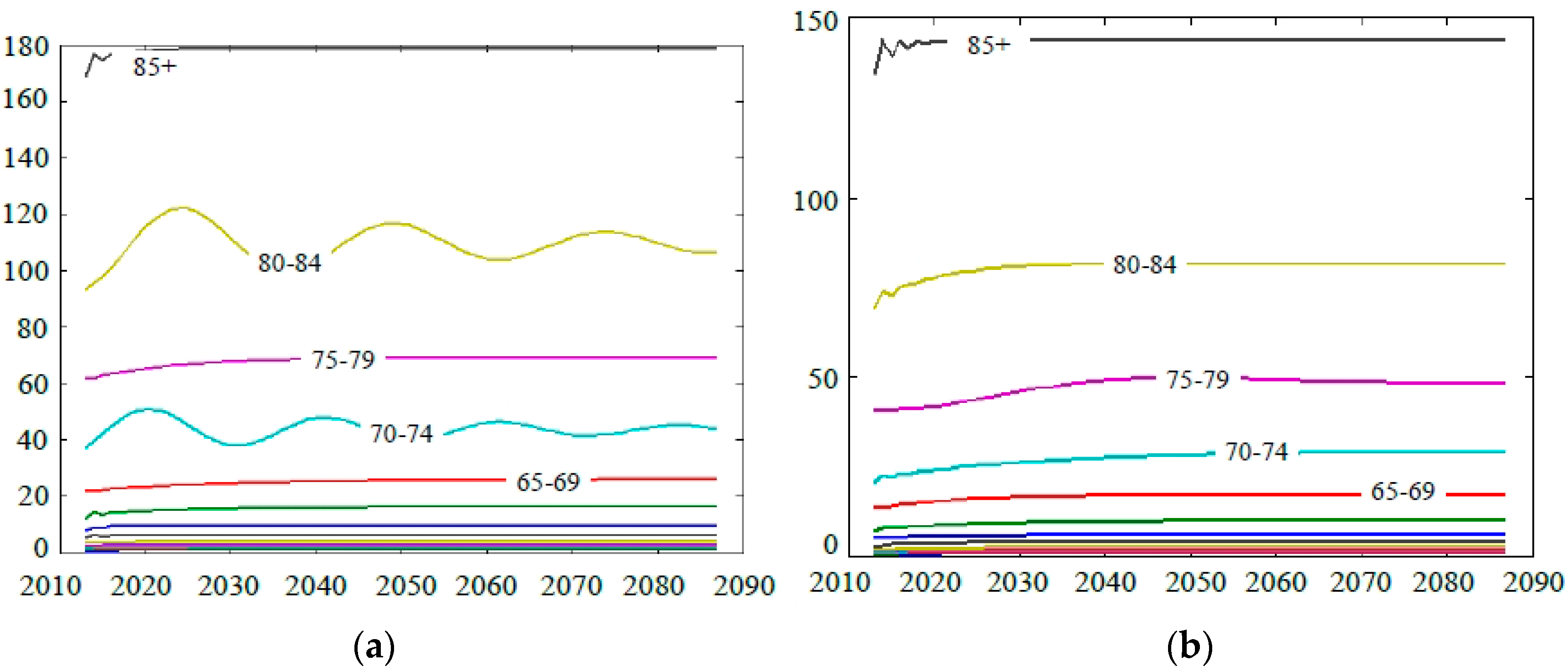
Time series models have the advantage of being stochastic, enabling the calculation of the probabilistic prediction interval for the forecast value, but a major disadvantage of such an approach is that the independent forecasting of mortality at each age may lead to implausible age patterns, especially in the long run [30]. Figure 2a,b show the age patterns of male mortality and female mortality after age 20, separately. Notice that the age patterns of male mortality and female mortality aged 20–50 are too narrow to resolve the age value. We can see that mortality rates for all simulations show a continual increase with age (after age 20), which indicates that their age patterns of mortality do not yield odd patterns by age.

Figure 2. (a) Age patterns of male mortality after age 20; (b) Age patterns of female mortality after age 20.

Figure 2. (a) Age patterns of male mortality after age 20; (b) Age patterns of female mortality after age 20.

(ii) Fertility Rate. Age-specific fertility rates (‰) of women at childbearing ages are calculated for seven age groups (15–19, 20–24, 25–29, 30–34, 35–39, 40–44, and 45–49) in 1994–2013. Historical time-series annual data can be obtained from the National Bureau of Statistics of the People’s Republic of China.

The same analysis approach is used and the ARMA(2,2) model is adopted to forecast the fertility rate. Table 4 shows the estimating equations of age-specific fertility rates.

Table 4. Time series estimating equations of age-specific fertility rates.

Age	Time Series Estimating Equations	${\overline{F}}_s$	$R^2$	$\sigma$
15–19	$F_{t,s}={\overline{F}}_s-0.0114f_{t-1,s}-0.0645f_{t-2,s}+{\mathsf{\epsilon }}_t+0.6121{\mathsf{\epsilon }}_{t-1}+0.1540{\mathsf{\epsilon }}_{t-2}$	5.1195	0.27	1.5653
20–24	$F_{t,s}={\overline{F}}_s+1.1055f_{t-1,s}-0.2821f_{t-2,s}+{\mathsf{\epsilon }}_t-0.2295{\mathsf{\epsilon }}_{t-1}+0.2688{\mathsf{\epsilon }}_{t-2}$	109.1060	0.84	11.3101
25–29	$F_{t,s}={\overline{F}}_s-0.3345f_{t-1,s}-0.0103f_{t-2,s}+{\mathsf{\epsilon }}_t+0.7694{\mathsf{\epsilon }}_{t-1}+0.9763{\mathsf{\epsilon }}_{t-2}$	104.0725	0.55	11.6693
30–34	$F_{t,s}={\overline{F}}_s+0.7494f_{t-1,s}+0.0222f_{t-2,s}+{\mathsf{\epsilon }}_t-0.1695{\mathsf{\epsilon }}_{t-1}-0.1531{\mathsf{\epsilon }}_{t-2}$	41.6465	0.52	5.6856
35–39	$F_{t,s}={\overline{F}}_s+0.5746f_{t-1,s}-0.0172f_{t-2,s}+{\mathsf{\epsilon }}_t+0.4756{\mathsf{\epsilon }}_{t-1}+0.8686{\mathsf{\epsilon }}_{t-2}$	12.3760	0.77	2.7875
40–44	$F_{t,s}={\overline{F}}_s+0.4756f_{t-1,s}+0.1367f_{t-2,s}+{\mathsf{\epsilon }}_t+0.5237{\mathsf{\epsilon }}_{t-1}+0.8911{\mathsf{\epsilon }}_{t-2}$	3.5620	0.82	1.2606
45–49	$F_{t,s}={\overline{F}}_s+1.6732f_{t-1,s}-0.8135f_{t-2,s}+{\mathsf{\epsilon }}_t-0.6098{\mathsf{\epsilon }}_{t-1}-0.2981{\mathsf{\epsilon }}_{t-2}$	1.8340	0.79	1.0541

Note: $F_{t,s}$—Female fertility rate aged s in year t; ${\overline{F}}_s$—Historical mean of female fertility rate aged s; $f_{t,s}$—Deviation of the female fertility rate aged s in year t from the historical mean, $f_{t,s}=F_{s,t}-{\overline{F}}_s$; $R^2$—R-squared value of the estimating equations; ${\mathsf{\epsilon }}_t$—Random error in year t.

Table 4. Time series estimating equations of age-specific fertility rates.

Age	Time Series Estimating Equations	${\overline{F}}_s$	$R^2$	$\sigma$
15–19	$F_{t,s}={\overline{F}}_s-0.0114f_{t-1,s}-0.0645f_{t-2,s}+{\mathsf{\epsilon }}_t+0.6121{\mathsf{\epsilon }}_{t-1}+0.1540{\mathsf{\epsilon }}_{t-2}$	5.1195	0.27	1.5653
20–24	$F_{t,s}={\overline{F}}_s+1.1055f_{t-1,s}-0.2821f_{t-2,s}+{\mathsf{\epsilon }}_t-0.2295{\mathsf{\epsilon }}_{t-1}+0.2688{\mathsf{\epsilon }}_{t-2}$	109.1060	0.84	11.3101
25–29	$F_{t,s}={\overline{F}}_s-0.3345f_{t-1,s}-0.0103f_{t-2,s}+{\mathsf{\epsilon }}_t+0.7694{\mathsf{\epsilon }}_{t-1}+0.9763{\mathsf{\epsilon }}_{t-2}$	104.0725	0.55	11.6693
30–34	$F_{t,s}={\overline{F}}_s+0.7494f_{t-1,s}+0.0222f_{t-2,s}+{\mathsf{\epsilon }}_t-0.1695{\mathsf{\epsilon }}_{t-1}-0.1531{\mathsf{\epsilon }}_{t-2}$	41.6465	0.52	5.6856
35–39	$F_{t,s}={\overline{F}}_s+0.5746f_{t-1,s}-0.0172f_{t-2,s}+{\mathsf{\epsilon }}_t+0.4756{\mathsf{\epsilon }}_{t-1}+0.8686{\mathsf{\epsilon }}_{t-2}$	12.3760	0.77	2.7875
40–44	$F_{t,s}={\overline{F}}_s+0.4756f_{t-1,s}+0.1367f_{t-2,s}+{\mathsf{\epsilon }}_t+0.5237{\mathsf{\epsilon }}_{t-1}+0.8911{\mathsf{\epsilon }}_{t-2}$	3.5620	0.82	1.2606
45–49	$F_{t,s}={\overline{F}}_s+1.6732f_{t-1,s}-0.8135f_{t-2,s}+{\mathsf{\epsilon }}_t-0.6098{\mathsf{\epsilon }}_{t-1}-0.2981{\mathsf{\epsilon }}_{t-2}$	1.8340	0.79	1.0541

Note: $F_{t,s}$—Female fertility rate aged s in year t; ${\overline{F}}_s$—Historical mean of female fertility rate aged s; $f_{t,s}$—Deviation of the female fertility rate aged s in year t from the historical mean, $f_{t,s}=F_{s,t}-{\overline{F}}_s$; $R^2$—R-squared value of the estimating equations; ${\mathsf{\epsilon }}_t$—Random error in year t.

3.1.2. Wage Parameter

The average wage of urban workers is:

$$W_t=W_{t-1}\times (1+G_t),$$

(10)

where

$G_t$—Growth rate of average wage in year t.

Historical time-series annual data for the growth rate of the average wage of urban workers in China from 1953 to 2013 are available from the National Bureau of Statistics of the People’s Republic of China.

The same analysis approach is used and the AR(5) model is adopted to estimate the growth rate of urban workers’ average wage. The R-square value is 0.74 and the estimating equation of the growth rate of average wage is:

$$G_t={\overline{G}}_t+0.6403g_{t-1}+0.0693g_{t-2}-0.1707g_{t-3}+0.1818g_{t-4}+0.1014g_{t-5}+{\epsilon }_t,$$

(11)

where

${\overline{G}}_t$—Historical mean of the growth rate of the average wage of urban workers in year t; it is 8.3727%;

$g_t$—Deviation of the growth rate of the average wage of urban workersin year t from the historical mean, $g_t=G_t-{\overline{G}}_t$;

${\mathsf{\epsilon }}_t$—Random error in year t.

3.2. Parameter Estimation

The population can be calculated iteratively by using the initial population adding births and subtracting deaths to age-specific population in the year. This paper constructs a Leslie transfer matrix [36] with fertility rate, mortality rate, and sex rate at birth, then uses the Monte Carlo stochastic simulation method to predict the evolution of the population [37,38].

The population is divided into 36 age-sex groups (0–4, 5–9, 10–14, …, 75–79, 80–84, 85+; male and female). Suppose that the initial population is:

$$PO{P}^{(0)}={(PO{P}_0^f,PO{P}_5^f,\dots ,PO{P}_{80}^f,PO{P}_{85+}^f,PO{P}_0^m,PO{P}_5^m,\dots ,PO{P}_{80}^m,PO{P}_{85+}^m)}_{36\times 1}^T$$

(12)

where

POP⁽⁰⁾—initial population, superscript (0) represents the starting-point of prediction, superscript $f$ represents female, superscript $m$ represents male.

For any age group with a period of five years, the predicted values of the mortality rate D in the age group can be estimated using the above time series models. Then the predicted values of the survival rate may be expressed as 1-D during the same period.

The matrix S^f of the female survival rate is:

$$S^f={\left[\begin{array}{cccccc}0& \cdots & \cdots & \cdots & \cdots & 0\\ 1-D_0^f& & & & & \\ & 1-D_5^f& & & & \\ & & \ddots & & & \\ & & & \ddots & & \\ & & & & 1-D_{80}^f& 1-D_{85+}^f\end{array}\right]}_{18\times 18}.$$

(13)

The matrix S^m of the male survival rate is:

$$S^m={\left[\begin{array}{cccccc}0& \cdots & \cdots & \cdots & \cdots & 0\\ 1-D_0^m& & & & & \\ & 1-D_5^m& & & & \\ & & \ddots & & & \\ & & & \ddots & & \\ & & & & 1-D_{80}^m& 1-D_{85+}^m\end{array}\right]}_{18\times 18}.$$

(14)

The matrix B^f of the female birth rate is:

$$B^f={\left[\begin{array}{ccccc}{b}_0^f& b_5^f& \cdots & b_{80}^f& b_{85+}^f\\ 0& 0& \cdots & 0& 0\\ ⋮& ⋮& ⋮& ⋮& ⋮\\ 0& 0& \cdots & 0& 0\end{array}\right]}_{18\times 18}.$$

(15)

The matrix B^m of the male birth rate is:

$$B^m={\left[\begin{array}{ccccc}{b}_0^m& b_5^m& \cdots & b_{80}^m& b_{85+}^m\\ 0& 0& \cdots & 0& 0\\ ⋮& ⋮& ⋮& ⋮& ⋮\\ 0& 0& \cdots & 0& 0\end{array}\right]}_{18\times 18}.$$

(16)

Obviously, each element in the first line of matrix B^f corresponds to that of matrix B^m. Suppose that F_s represents the fertility rate of any age group and BR represents the birth rate of baby boys. Thus, the relevant elements of a birth matrix can be calculated by the following equations: $b_s^m=BR\times F_s$, $b_s^f=(1-BR)\times F_s$.

Based on the fertility rate, mortality rate, and sex rate at birth, the Leslie transfer matrix L is:

(17)

The five-year population can be forecasted by the following equation:

$$P^{(5)}=L^{(5)}\times P^{(0)}.$$

(18)

By iterative method, Equation(18) can be extended as follows:

$$P^{(n+5)}=L^{(n+5})\times P^{(n)},$$

(19)

where

$P^{(n+5)}$—Population in n+5 year;

$L^{(n+5)}$—Leslie transfer matrix in n+5 year;

$P^{(n)}$—Population in n year.

Through the independent implementation of Monte Carlo simulations many times, we obtain the distribution of population $P^{(n+5)}$. Figure 3 and Figure 4 show the estimated probability intervals of the total population size and the proportion of the elderly population aged over 60, respectively. Notice that the smooth curves do not represent the path of any particular simulation. Instead, for each given year, the curves represent the distribution of prediction parameters based on all stochastic simulation results for that year. The two extreme curves in the figures comprise a 95-percent probability interval, and deciles are shown for the range of the 10th through the 90th percentiles. The simulation result indicates that the total population increases slightly from 2013 to 2022 and then decreases continuously. Meanwhile, the median value of the total population is 1418.56 million in 2015 and 1414.86 million in 2030. In 2050, there is a 90% chance that the total population is 1350.44 million. On these same plots, the official UN forecasts for the total population in China are 1376.04 million, 1415.54 million, and 1348.05 million, respectively [39].

Figure 3. Total population size.

Figure 3. Total population size.

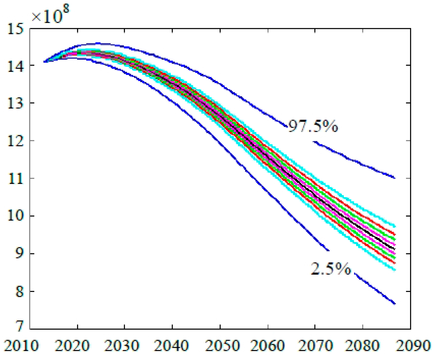
Figure 4. The proportion of the elderly population.

Figure 4. The proportion of the elderly population.

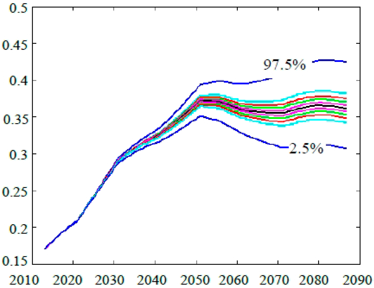
Figure 4 shows that the proportion of the population aged over 60 will increase quickly from 2013 to 2050 and then slowly decline from 2051 to 2071. After 2072, it will slowly rise again. The median value of the population aged over 60 is 15.68% in 2015 and 36.53% in 2050. On these same plots, the official UN forecasts for the proportion of the population aged over 60 in China are 15.2% and 36.5% [39]. Both forecast results are very close.

(1) Number of insured employees

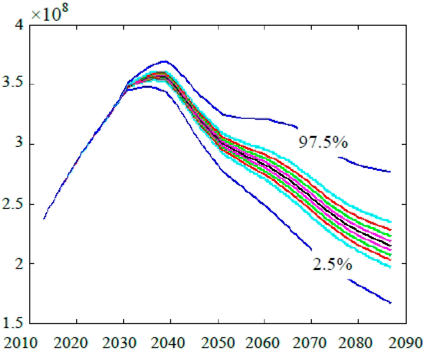
The number of insured employees directly determines the contributions of the basic pension. Figure 5 shows the estimated probability intervals of the annual number of insured employees. The two extreme curves in the figure comprise a 95-percent probability interval, and deciles are shown for the range of the 10th through the 90th percentiles. The number of insured employees increases quickly at first, culminating with a median value of 369.81 million in 2038, and then decreases continuously.

Figure 5. Number of insured employees.

Figure 5. Number of insured employees.

(2) Number of pensioners

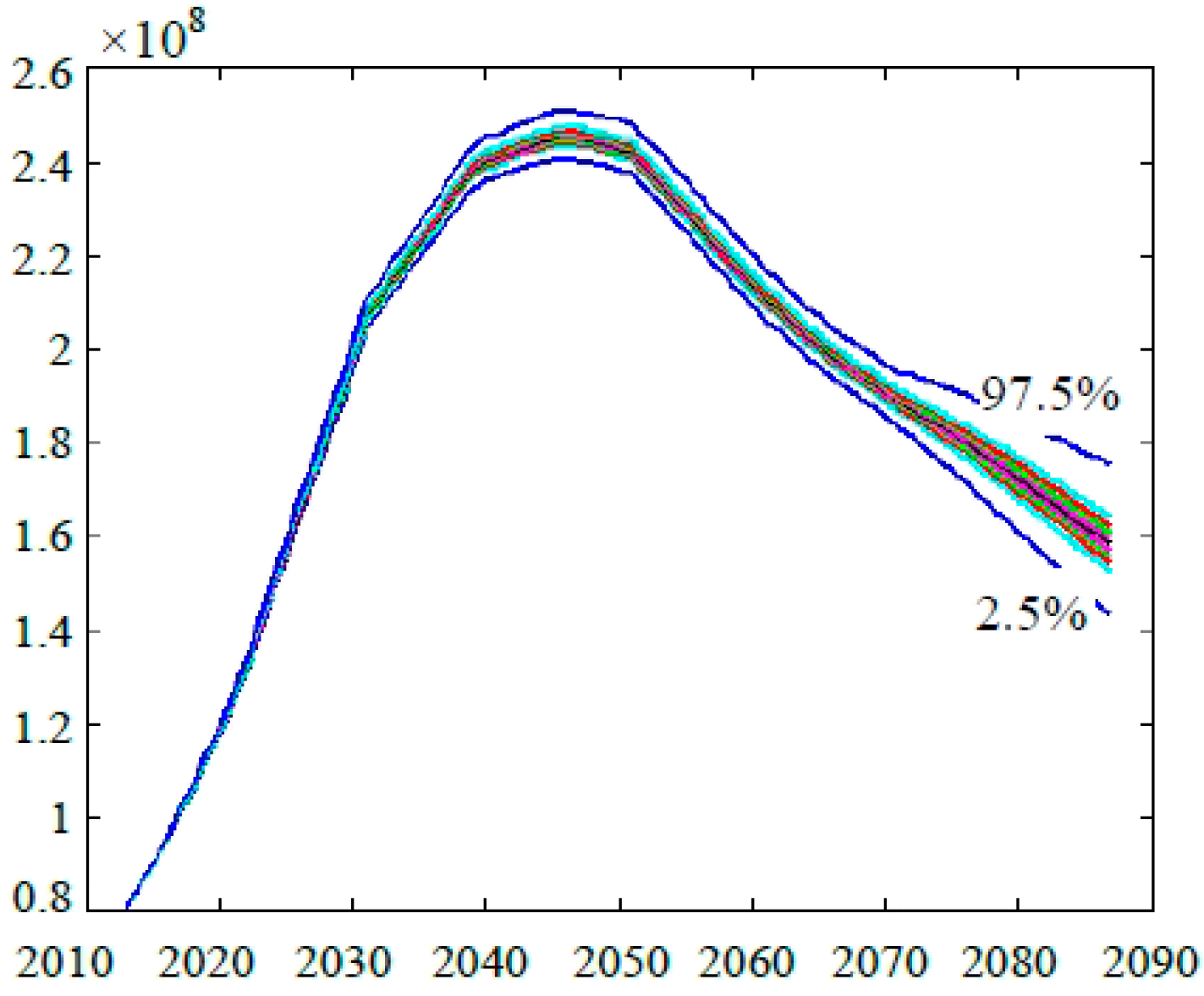
The number of pensioners directly determines the expenditures on the basic pension. Figure 6 shows the estimated probability intervals of the annual number of pensioners. As before, the two extreme curves in the figure comprise a 95-percent probability interval, and deciles are shown for the range of the 10th through the 90th percentiles. As shown in Figure 6, the number of pensioners increases quickly from 2013 to 2032. Then it shows a decelerated upward evolution from 2033 to 2052, culminating with a median value of 246.54 million in 2046. After 2053, the number of pensioners decreases year by year.

Figure 6. Number of pensioners.

Figure 6. Number of pensioners.

(3) Average wage of urban workers

The annual average wage of urban workers affects the contributions and expenditures of the basic pension. Figure 7 shows the estimated probability intervals of the annual average wage of urban workers. As before, the two extreme curves in the figure comprise a 95-percent probability interval, and deciles are shown for the range of the 10th through the 90th percentiles. As shown in Figure 7, the average wage of urban workers increases steadily over the following 75 years. The median value increases from 52,308 Yuan (the actual value was about 51,483 Yuan) in 2013 to 5.6238 million Yuan in 2087.

Figure 7. Average wage of urban workers.

Figure 7. Average wage of urban workers.

4. Simulation Results

The Monte Carlo stochastic simulation method is carried out based on the above parameter estimation and assumption. Through 5000 times of simulation, the dynamic processes of the financial sustainability of the basic pension over the next 75 years are shown as follows.

4.1. Contributions of the Basic Pension

Figure 8 shows the estimated probability intervals of the annual contributions of the basic pension from 2013 to 2087. As before, the two extreme curves in the figure comprise a 95-percent probability interval, and deciles are shown for the range of the 10th through the 90th percentiles. It should be noted that the results of the smooth curves do not represent the path of any particular simulation. Instead, for each given year, the curved lines represent the distribution of the contributions of the basic pension based on all stochastic simulation results for that year. As shown in Figure 8, contributions to the basic pension increase rapidly during the forecast period and the median estimation of contributions increases from 2.197 trillion Yuan (the real contribution is 2.268 trillion Yuan) in 2013 to 148.12 trillion Yuan in 2087.

Figure 8. Contributions of basic pension.

Figure 8. Contributions of basic pension.

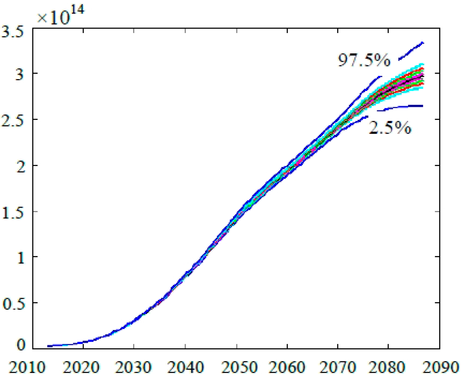
4.2. Expenditures of the Basic Pension

Figure 9 shows the estimated probability intervals of the annual expenditures of the basic pension from 2013 to 2087. As before, the two extreme curves in the figure comprise a 95-percent probability interval, and deciles are shown for the range of the 10th through the 90th percentiles. According to the results, the expenditures of the basic pension from 2013 to 2052 increase quickly, while from 2053 to the end of the forecast period the growth of the expenditures becomes slower. During the forecast period, the expenditures of the basic pension are on the rise, and the median forecast of expenditures goes up from 1.8032 trillion Yuan (the real expenses are 1.847 trillion Yuan) in 2013 to 298.02 trillion Yuan in 2087.

Figure 9. Expenditures of the basic pension.

Figure 9. Expenditures of the basic pension.

4.3. Cumulative Balance of the Basic Pension

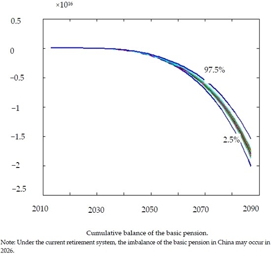
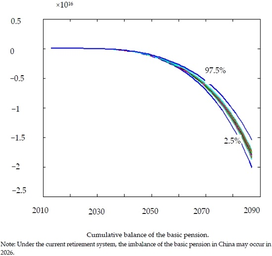
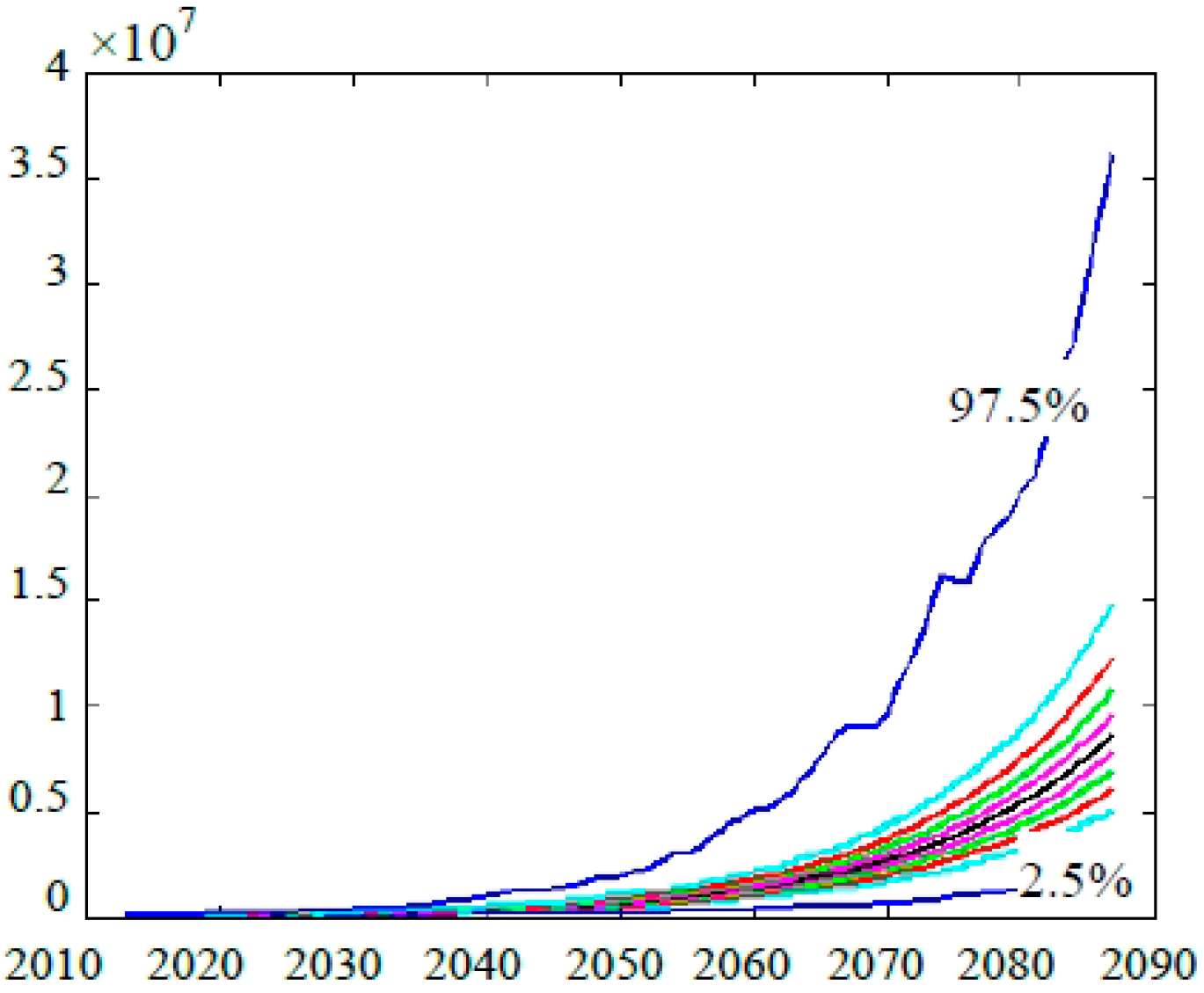
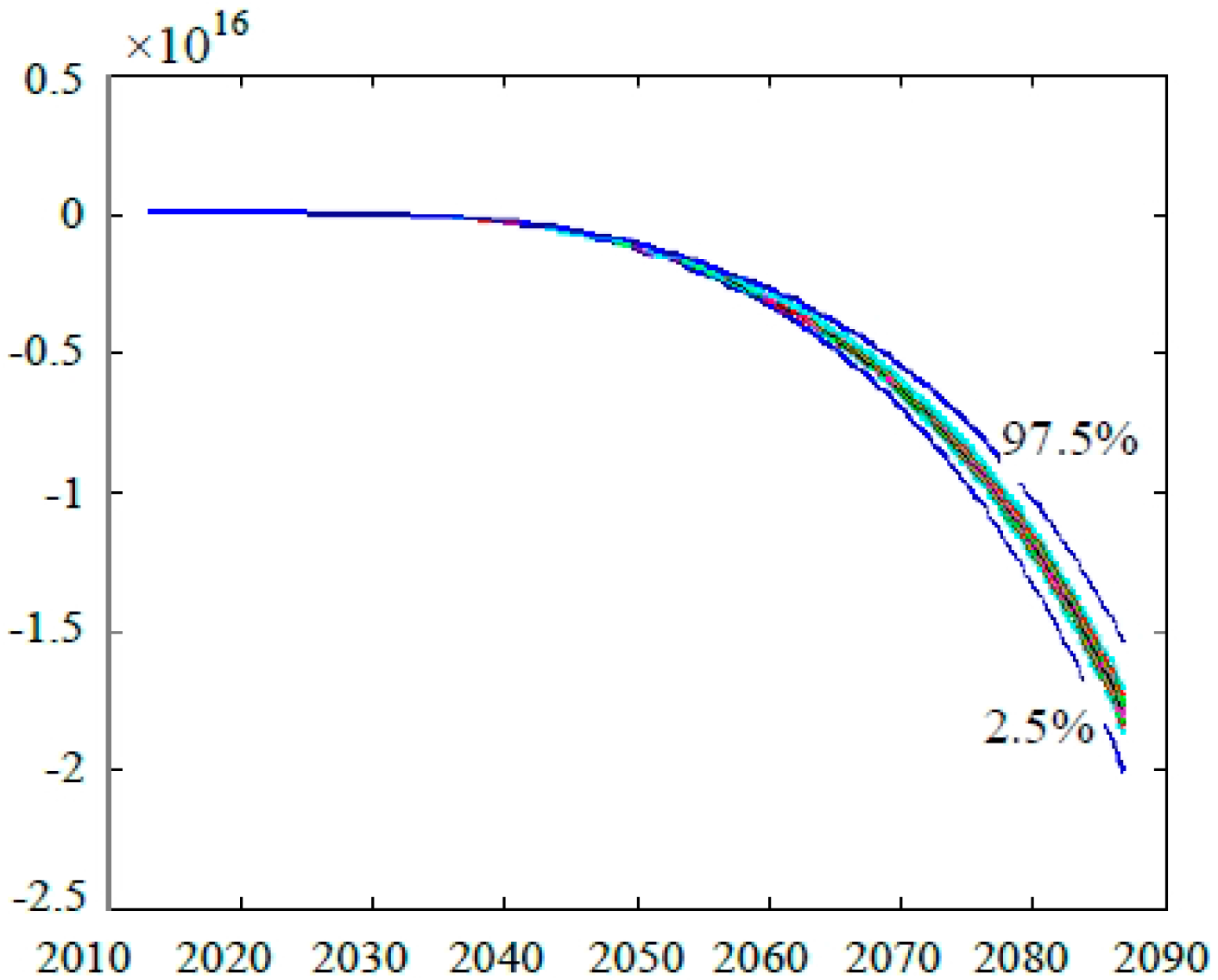
Figure 10 shows the estimated probability intervals of the annual cumulative balance of the basic pension from 2013 to 2087. As before, the two extreme curves in the figure comprise a 95-percent probability interval, and deciles are shown for the range of the 10th through the 90th percentiles. It shows that the basic pension from 2013 and 2025 is profitable, and the median forecast of the cumulative balance of the basic pension increases slowly from 2.8573 trillion Yuan (the real cumulative balance is 2.8269 trillion Yuan) to 7.3516 trillion Yuan; then it declines. There is a 95% chance that the system could become insolvent in 2026. At the same time, the median deficit will increase from 1.8869 trillion Yuan in 2026 to 1795.12 trillion Yuan in 2087.

Figure 10. Cumulative balance of the basic pension.

Figure 10. Cumulative balance of the basic pension.

5. Effect of the Delay of Retirement on Pension Sustainability

The retirement age is the key factor affecting the balance of the pension payment [40,41]. The delay of retirement is conducive to increasing the contributions and decreasing the expenditures of the basic pension. Therefore, it would be useful in relieving the financial imbalance of pension payment and reducing the possibility of a pension payment gap. In 2013, the third session of the 18th Conference of the Chinese Communist Party adopted a decision that China would raise the retirement age in progressive steps. Moreover, the Ministry of Human Resources and Social Security of China also pointed out that the policy of postponing retirement age would be approved before 2020.

Under the assumption that other things remain equal, suppose that the retirement age is raised from 55 to 60 for women and from 60 to 65 for men. Then, using the Monte Carlo method, the dynamic process of the financial sustainability of the basic pension over the next 75 years was stochastically simulated again.

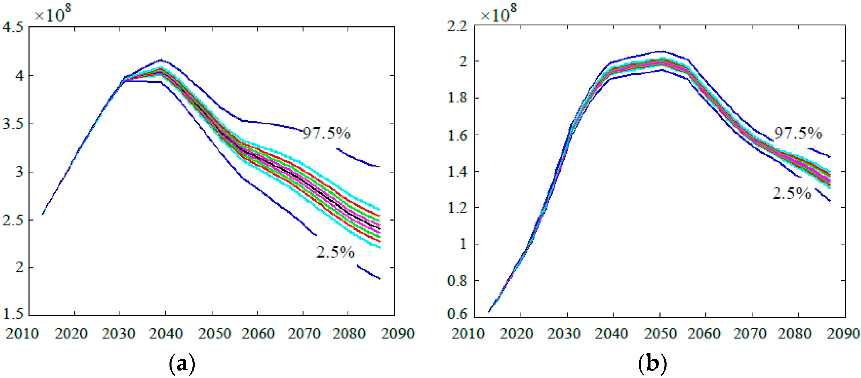
Figure 11a,b show the estimated probability intervals of the number of insured employees and pensioners under the assumption of raising the retirement age. As before, the two extreme curves in the figure comprise a 95-percent probability interval, and deciles are shown for the range of the 10th through the 90th percentiles. Compared with the previous predictions, these changing trends of the population are roughly the same, whereas the degree of variations is different. Furthermore, with the delay of retirement by five years, the median value of the number of insured employees will increase by about 10%, and the number of pensioners will decrease by about 30% at the same time.

Figure 11. (a) Number of insured employees under the assumption of postponing the retirement age by five years; (b) Number of pensioners under the assumption of postponing the retirement age by five years.

Figure 11. (a) Number of insured employees under the assumption of postponing the retirement age by five years; (b) Number of pensioners under the assumption of postponing the retirement age by five years.

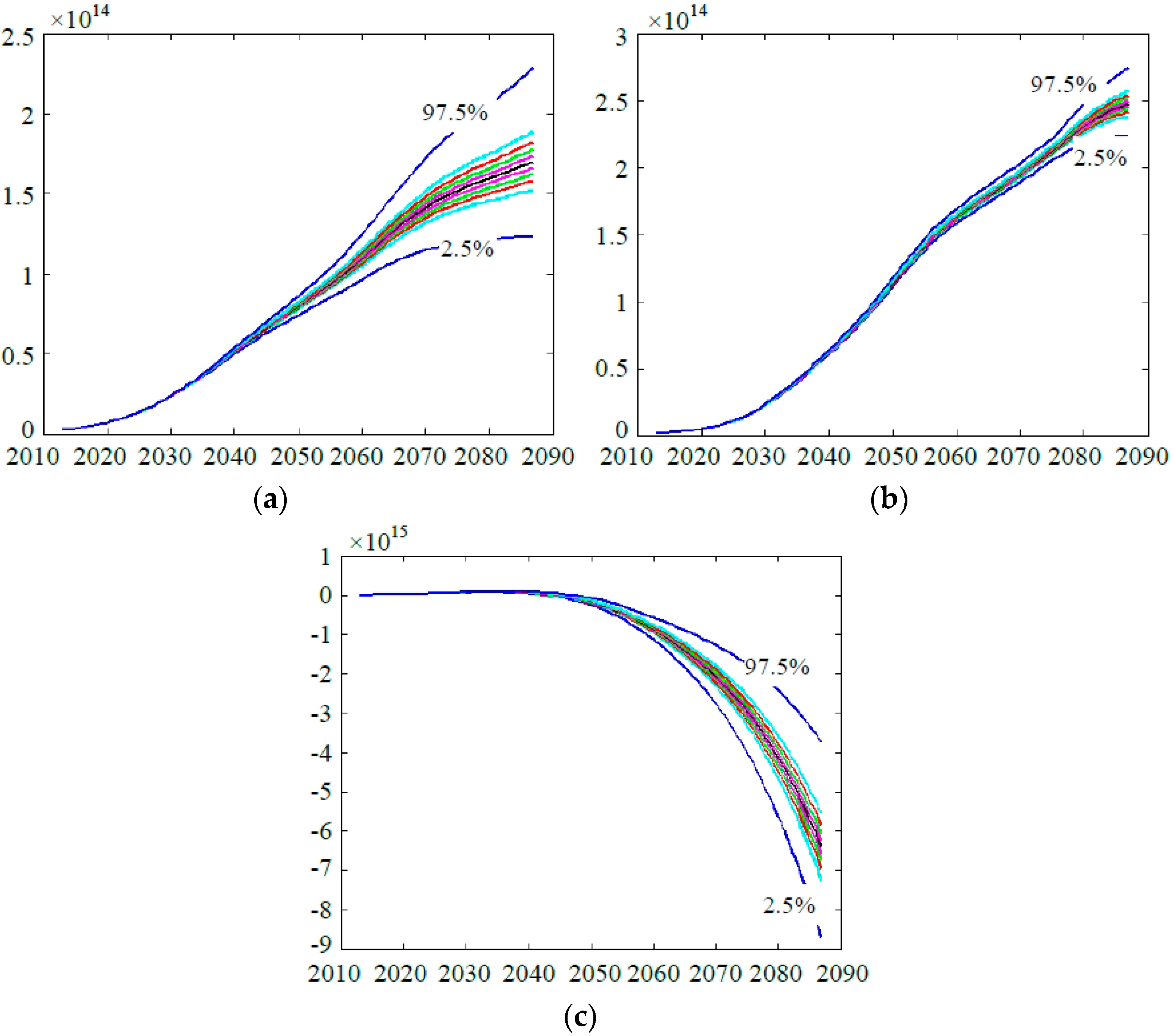
Figure 12a–c show the estimated probability intervals of the contributions, expenditures, and cumulative balance of the basic pension under the assumption of raising the retirement age. As before, the two extreme curves in the figure comprise a 95-percent probability interval, and deciles are shown for the range of the 10th through the 90th percentiles. Compared with previous predictions, the changing tendencies of the financial status of the basic pension are also roughly the same, whereas their values change substantially. With the delay of retirement by five years, the median value of the contributions of the basic pension will increase by about 10%, and the expenditures of the basic pension will decrease by about 30%. As shown in Figure 12c, there is a 10% chance that the basic pension system will become insolvent in 2044, 70% in 2045, and 90% in 2046. This indicates that the occurrence of financial deficit of the basic pension will be postponed by about 20 years. Moreover, at the end of the forecast period, the median cumulative deficit is about 641.7 trillion Yuan, which is reduced by more than 64.25%.

Figure 12. (a) Contributions to the basic pension under the assumption of postponing the retirement age by five years; (b) expenditures of the basic pension under the assumption of postponing the retirement age by five years; (c) cumulative balance of the basic pension under the assumption of postponing the retirement age by five years.

Figure 12. (a) Contributions to the basic pension under the assumption of postponing the retirement age by five years; (b) expenditures of the basic pension under the assumption of postponing the retirement age by five years; (c) cumulative balance of the basic pension under the assumption of postponing the retirement age by five years.

6. Conclusions

This paper stochastically simulated the financial sustainability of the basic pension. The predicted results above illustrate that the basic pension will face unprecedented payment pressure. With the fast aging process, an imbalance of the basic pension will occur in 2026 and the median deficit will be 1.8869 trillion Yuan. Then, the financial gap will expand year by year. Therefore, we suggest that the Chinese government should adopt a stable and long-term fiscal subsidy policy to fill the huge gap the basic pension will experience in the future. Furthermore, the special fund reserved for pension payments is helpful for achieving the financial sustainability of the basic pension.

It is also found that if the government postpones the retirement age by five years (for both men and women), the occurrence of financial deficit of the basic pension may be postponed by about 20 years and the median cumulative deficit will also be reduced by more than 64.25% in 2087. In the end, the delay of retirement in China is inevitable as a way of dealing with the population aging. Meanwhile, it is also an effective method of relieving the enormous pressure on payments of the basic pension. Therefore, the reformation of endowment insurance system should be broadened and the top-design of progressively raising the retirement age should be finished as soon as possible in accordance with the current economy, population, employment, and other actualities of China.

References

- Dorfman, M.; Holzmann, R.; O’Keefe, P.; Wang, D.W.; Sin, Y.; Hinz, R. China’s Pension System : A Vision; World Bank Publications: Washington, DC, USA, 2013. [Google Scholar]
- European Commission. Adequate and Sustainable Pensions, Joint Report of the Commission and the Council; Official Publications of the European Communities: Brussels, Beligum, 2003. [Google Scholar]
- Holzmann, R.; Hinz, R.; von Gersdorff, H.; Gill, I.; Impavido, G.; Musalem, A.R.; Rutkowski, M.; Palacios, R.; Sin, Y.; Subbarao, K.; et al. Old-Age Income Support in the Twenty-first Century: An International Perspective on Pension Systems and Reform; World Bank Publications: Washington, DC, USA, 2005. [Google Scholar]
- Grech, A.G. Assessing the Sustainability of Pension Reforms in Europe; London School of Economics & Political Science: London, UK, 2010. [Google Scholar]
- Pânzaru, C. Some Considerations of Population Dynamics and the Sustainability of Social Security System. Procedia Soc. Behav. Sci. 2015, 183, 68–76. [Google Scholar] [CrossRef]
- Roseveare, D.; Leibfritz, W.; Fore, D.; Wurzel, E. Ageing Populations, Pension Systems and Government Budgets: Simulations for 20 OECD Countries; Economics Department Working Papers No. 168; The Organisation for Economic Co-operation and Development (OECD) iLibrary: Paris, France, 1996. [Google Scholar]
- Petersen, J.H. Recent research on public pension systems. A review. Labour Econ. 1998, 5, 91–108. [Google Scholar] [CrossRef]
- Andersen, T.M. Increasing longevity and social security reforms—A legislative procedure approach. J. Public Econ. 2008, 92, 633–646. [Google Scholar] [CrossRef]
- Heijdra, B.; Romp, W. Retirement, pensions, and ageing. J. Public Econ. 2009, 93, 586–604. [Google Scholar] [CrossRef]
- Kaganovich, M.; Zilcha, I. Pay-as-you-go or funded social security? A general equilibrium comparison. J. Econ. Dyn. Control 2012, 36, 455–467. [Google Scholar] [CrossRef]
- Lee, R.; Tuljapurkar, S. Stochastic Forecasts for Social Security. Front. Econ. Aging 1998, 1, 393–428. [Google Scholar]
- Lee, R.; Yamagata, H. Sustainable Social Security: What Would It Cost? Natl. Tax J. 2003, 56, 27–43. [Google Scholar] [CrossRef]
- Lee, R.; Miller, T.; Anderson, M. Stochastic Infinite Horizon Forecasts for Social Security and Related Studies; NBER Working Paper No. 10917; The National Bureau of Economic Research: Cambridge, MA, USA, 2004. [Google Scholar]
- Social Security Administrate, Office of the Chief Actuary. A Stochastic Model of the Long-Range Financial Status of the OASDI Program; Actuarial Study No. 117; Social Security Administrate, Office of the Chief Actuary: Baltimore, MD, USA, 2004. [Google Scholar]
- World Bank. Averting the Old Age Crisis: Policies to Protect the Old and Promote Growth; World Bank Publications: Washington, DC, USA, 1994. [Google Scholar]
- Williamson, J.; Price, M.; Shen, C. Pension policy in China, Singapore, and South Korea: An assessment of the potential value of the notional defined contribution model. J. Aging Stud. 2012, 26, 79–89. [Google Scholar] [CrossRef]
- Wang, L.; béland, D.; Zhang, S. Pension financing in China: Is there a looming crisis? China Econ. Rev. 2014, 30, 143–154. [Google Scholar] [CrossRef]
- Wang, X.; Ren, W. Studies on the Financial Sustainability of Social Pension System in China. Insur. Stud. 2013, 4, 118–127. [Google Scholar]
- Zhao, B.; Yuan, H. The Analysis of Financial Balance and Sustainability for China’s Basic Pension: Based on the Perspective of Rational Fiscal Payment. Financ. Econ. 2013, 7, 38–46. [Google Scholar]
- Liu, X. Study on the Financing Gap and Sustainability of China’s Pension System. China Ind. Econ. 2014, 9, 25–37. [Google Scholar]
- Zhang, X.; Shi, L. Sustainability of Pension System and Public Debt in An Overlapping Generation Model. Nankai Econ. Stud. 2014, 2, 136–152. [Google Scholar]
- Feng, T.; Gao, X. A Simulation Study on the Sustainability of Rural Pension Based on Parameters Adjusting of Actuarial Models. Chin. J. Manag. Sci. 2015, 9, 153–161. [Google Scholar]
- Ding, S.; Wang, X. A Study on Rural Aging and Sustainable Old-age Security System in China. Econ. Issues China 2012, 2, 52–60. [Google Scholar]
- Feng, T.; Gao, X. The Population Aging Impact on the Sustainability of Rural Pension: An Empirical Study Based on VAR Model. Manag. Rev. 2015, 6, 30–41. [Google Scholar]
- Yu, H.; Zhong, H. On Sustainable Operation of China’s Basic Pension Insurance System: Analysis of Three Simulation Conditions. J. Financ. Econ. 2009, 9, 26–35. [Google Scholar]
- Research Group of National Population Development Strategy. National Population Development Strategy Research. J. China Popul. Res. 2007, 31, 1–10. (In Chinese) [Google Scholar]
- Yang, H. How to Improve the Investment and Operation Mechanism on the Basic Old-age Insurance Fund. J. Cent. Univ. Financ. Econ. 2012, 9, 7–11. [Google Scholar]
- Zhou, P. An Exploration into the Business Model of Basic Pension Insurance Fund Investment and Operation--Based on the Perspective of Three-dimension Value. J. Liaoning Univ. Philos. Soc. Sci. 2015, 1, 99–104. [Google Scholar]
- Jimeno, J.; Rojas, J.; Puente, S. Modelling the impact of aging on social security expenditures. Econ. Model. 2008, 25, 201–224. [Google Scholar] [CrossRef]
- Booth, H.; Tickle, L. Mortality Modelling and Forecasting: A Review of Methods. Ann. Actuar. Sci. 2008, 1–2, 3–43. [Google Scholar]
- Bell, W.R. Comparing and Assessing Time Series Methods for Forecasting Age-specific Fertility and Mortality rates. J. Off. Stat. 1997, 3, 279–303. [Google Scholar]
- Lee, R.; Tuljapurkar, S. Population Forecasting for Fiscal Planning: Issues and Innovations; Burch Working Paper No. B98–05; University of California: Berkeley, CA, USA, 1998. [Google Scholar]
- Lutz, W.; Sanderson, W.C.; Scherbov, S. Expert-based Probabilistic Population Projections. Popul. Dev. Rev. 1998, 24, 139–155. [Google Scholar] [CrossRef]
- Lutz, W.; Sanderson, W.C.; Scherbov, S. The End of World Population Growth. Nature 2001, 412, 543–545. [Google Scholar] [CrossRef] [PubMed]
- Ren, Q.; Hou, D. Stochastic Model for Population Forecast: Based on Leslie Matrix and ARMA Model. Popul. Res. 2011, 2, 28–42. [Google Scholar]
- Keyfitz, N.; Caswell, H. Applied Mathematical Demography, 3rd ed.; Springer: New York, NY, USA, 2005. [Google Scholar]
- Mielczarek, B. Simulation model to forecast the consequences of changes introduced into the 2nd pillar of the Polish pension system. Econ. Model. 2013, 30, 706–714. [Google Scholar] [CrossRef]
- MacDonald, B.; Cairns, A. Three retirement decision models for defined contribution pension plan members: A simulation study. Insur. Math. Econ. 2011, 48, 1–18. [Google Scholar] [CrossRef]
- United Nations. Department of Economic and Social Affairs. World Population Prospects: The 2015 Revision, Key Findings and Advance Tables; Working Paper No. ESA/P/WP.241; United Nations: New York, NY, USA, 2015. [Google Scholar]
- Martín, A. Endogenous retirement and public pension system reform in Spain. Econ. Model. 2010, 27, 336–349. [Google Scholar] [CrossRef]
- Galasso, V. Postponing retirement: The political effect of aging. J. Public Econ. 2008, 92, 2157–2169. [Google Scholar] [CrossRef]
© 2016 by the authors; licensee MDPI, Basel, Switzerland. This article is an open access article distributed under the terms and conditions of the Creative Commons by Attribution (CC-BY) license (http://creativecommons.org/licenses/by/4.0/).
Share and Cite
MDPI and ACS Style
Tian, Y.; Zhao, X. Stochastic Forecast of the Financial Sustainability of Basic Pension in China. Sustainability 2016, 8, 46. https://doi.org/10.3390/su8010046
AMA Style
Tian Y, Zhao X. Stochastic Forecast of the Financial Sustainability of Basic Pension in China. Sustainability. 2016; 8(1):46. https://doi.org/10.3390/su8010046
Chicago/Turabian StyleTian, Yuehong, and Xianglian Zhao. 2016. "Stochastic Forecast of the Financial Sustainability of Basic Pension in China" Sustainability 8, no. 1: 46. https://doi.org/10.3390/su8010046
Note that from the first issue of 2016, this journal uses article numbers instead of page numbers. See further details here.