Analysis of Geo-Temperature Restoration Performance under Intermittent Operation of Borehole Heat Exchanger Fields

Abstract

Intermittent operation can improve the coefficient of performance (COP) of a ground source heat pump (GSHP) system. In this paper, an analytical solution to analyze the geo-temperature restoration performance under intermittent operation of borehole heat exchanger (BHE) fields is established. For this purpose, the moving finite line source model is combined with the g-function and the superposition principle. The model takes into account the heat transfer along the borehole, thermal interference between BHEs, and the influence of groundwater flow. The accuracy of the model is validated through comparison with an experiment carried out under intermittent operation. The model makes it possible to analyze the geo-temperature restoration performance and its influencing factors, such as BHE spacing, heat flow rate, operation mode, and groundwater flow. The main conclusions of this work are as follows. The heat transfer along the borehole should be considered when analyzing the geo-temperature restoration performance. When the BHE spacing increases, the soil temperature change decreases and the heat recovery improves. Therefore, adequate borehole separation distance is essential in the case of a multiple BHE system with unbalanced load. The presence of groundwater flow is associated with interference between the BHEs, which should not be ignored. In the case of long-term operation, the groundwater flow is beneficial to the geo-temperature recovery process, even for downstream BHEs. Finally, a greater groundwater flux leads to a better geo-temperature recovery.

1. Introduction

The use of geothermal energy in space conditioning of buildings has increased rapidly during the past several decades. This is achieved through the utilization of ground source heat pumps (GSHP). Compared to conventional air conditioning systems, GSHP can offer higher energy efficiency for air-conditioning [1,2,3,4], as they provide lower temperatures for cooling, higher temperatures for heating, and smaller temperature fluctuations than the ambient air temperature changes. Because of these advantages, more and more underground projects use GSHP. However, the load in the underground projects is usually unbalanced, especially in southern China where the cooling load is much greater than the heating load. This imbalance reduces the geothermal potential of the heat sink associated with the heat pump units [5,6]. This causes a decrease of the GSHP efficiency, and can eventually lead to a halt [7,8]. In this connection, the ASHRAE manual [9] was the first to discuss the advantages of a hybrid ground source heat pump (HGSHP) system, which uses a cooling tower as a supplemental heat rejecter. Significant research has been done by now on the application of HGSHP systems [10,11]. While promising, these systems are characterized by an increased complexity when running and maintaining GSHP [12]. Also, in some underground projects with special purposes, cooling towers are not recommended. Studies show that intermittent operation of the GSHP can reduce the heat accumulation in the vicinity of BHEs [13], which can improve to some degree the coefficient of performance (COP) of the pump. Therefore, more sophisticated models are required to predict the temperature changes under intermittent operation, so as to assure reasonable operation of the heat pump, and to avoid low performance due to heat transfer attenuation.

Over the years, many models have been developed for analyzing heat transfer in and around boreholes. This has been done using analytical, numerical, and hybrid methods. Classic analytical solutions include the line and cylindrical source models [14,15], which can provide results rather quickly. With the advent of computer science, numerical models have been rapidly developed, such as those based on finite difference, finite volume, and finite element methods [16,17]. The numerical models provide accurate solutions, but compared with the analytical methods, are of limited flexibility and time-consuming. Therefore, at present numerical models are rarely incorporated into simulation programs alone. The need to achieve both high precision and computational speed has led to hybrid models, a feasible alternative [18]. Such models are used to calculate special temperature response functions, which are then incorporated as databases into the simulation software. This type of software includes TRNSYS, Energy Plus, and GLEHEPRO [19].

In order to investigate the intermittent operation performance of a GSHP system, Cui et al. [20] developed a finite element numerical model for the GHEs in alternative operation modes. They found that the discontinuous operation mode and the alternative cooling/heating modes can effectively alleviate heat accumulation in the soil around BHEs, thus improving the performance of the system. Gao et al. [21] made a comparison of the energy efficiency in the case of a continuous operation versus intermittent control systems. Several factors were taken into account, such as thermal inertia, temperature levels, and lag time, in order to observe how they affect the efficiency. Shang et al. [22] presented a three-dimensional model to study influencing factors during the soil temperature recovery period, such as thermal conductivity, porosity, backfill material, air temperature, solar radiation, and wind velocity. The results reported by these authors show that the soil properties have a great impact on the heat recovery process. Signorelli [23] used 3D numerical models to study the sustainability of single and multi-BHE fields. It was shown that for a single BHE field, the temperature change at 50-m depth and at a distance of 0.1 m from the BHE was smaller than 0.1 K, after a 24-year recovery period. The recovery period increases to 70 years for a multi-BHE field, with array spacing of 7.5 m. Lazzari et al. [24] investigated the long-term performance of both single- and multi-BHE fields, with a periodic heat load in a conduction-dominated heat transfer system. They concluded that an almost complete heat load compensation is needed in the case of an infinite square BHE field, even when the spacing between the individual BHEs is large (14 m). A similar study of under groundwater flow was carried out by Zanchini et al. [25]. These authors point out that the performance of a BHE field becomes more sustainable when the Peclet number increases. Dehkordi and Schincariol [26] used a fully discretized finite-element model to study the thermal recovery realized 25 years after the decommissioning of a geothermal heat pump system. It was found that groundwater flow is the most important factor in the process of thermal recovery, while the impact of thermal conductivity is relatively minor.

The main objective of this paper was to obtain an analytical solution to be used in the analysis of the performance of an intermittently operating BHE field, in terms of geo-temperature restoration, and with the consideration of the groundwater flow. This solution is obtained by combining the moving finite line source model with a g-function, while observing the superposition principle. The model takes into account the heat transfer along boreholes, thermal interference between BHEs, and the effect of groundwater flow. The model was validated through a comparison with an experiment that was carried out under the conditions of intermittent operation. By studying five years’ intermittent operation under heating mode, which involves four months in active mode and eight months idle in a year, the geo-temperature restoration performance and the factors influencing geo-temperature recovery in the BHE fields was analyzed by the model. This paper provides a reference for the rational utilization in underground projects of intermittently operating GSHP systems.

2. Modeling

According to the geothermal literature, the existing infinite line source model and cylindrical heat source models, applied with a constant heat load, may provide a satisfactory estimate of the temperature change in the vicinity of the BHEs during GSHP operation. However, it is still difficult to analyze the geo-temperature recovery process, due to discontinuous operation. In addition, studies show that the two methods may not be appropriate in all cases, because of the following three phenomena [27]: (1) the axial effect, which is very small for short and medium time scales, but should not be ignored for long-term operations; (2) thermal interference between boreholes where more than one borehole is used [28]; and (3) groundwater flow, particularly when Darcy’s velocity is larger than 10 e⁻⁸ m/s [29,30].

Molina-Giraldo et al. [31] calculated the flowing analytical solution for a moving finite line source model:

$$\Delta T_{\text{MFLS}}(x,y,z,\mathsf{\tau })=\frac{q_l}{2\mathsf{\pi }\mathsf{\lambda }}\exp \left[\frac{v_{T}x}{2\mathsf{\alpha }}\right]\left[{\displaystyle \underset{0}{\overset{H}{\int }}f(x,y,z,\mathsf{\tau })\text{d}h-{\displaystyle \underset{-H}{\overset{0}{\int }}f(x,y,z,\mathsf{\tau })\text{d}h}}\right]$$

(1)

where

$$\begin{array}{l}f(x,y,z,\mathsf{\tau })=\frac{1}{4r}[\exp (-\frac{v_T\sqrt{r^2+{(z-h)}^2}}{2\mathsf{\alpha }})erfc(\frac{\sqrt{r^2+{(z-h)}^2}-v_T\mathsf{\tau }}{2\sqrt{\mathsf{\alpha }\mathsf{\tau }}})+...\\ \exp (\frac{v_T\sqrt{r^2+{(z-h)}^2}}{2\mathsf{\alpha }})erfc(\frac{\sqrt{r^2+{(z-h)}^2}+v_T\mathsf{\tau }}{2\sqrt{\mathsf{\alpha }\mathsf{\tau }}})]\end{array}$$

$$\mathsf{\alpha }=\mathsf{\lambda }/\mathsf{\rho }c$$

$$\mathsf{\lambda }=\mathsf{\epsilon }{\mathsf{\lambda }}_{\text{w}}+\left(1-\mathsf{\epsilon }\right){\mathsf{\lambda }}_{\text{s}}$$

$$\mathsf{\rho }c=\mathsf{\epsilon }{\mathsf{\rho }}_{\text{w}}{c}_{\text{w}}+\left(1-\mathsf{\epsilon }\right){\mathsf{\rho }}_{\text{s}}{c}_{\text{s}}$$

and

$$v_T=u{\mathsf{\rho }}_{\text{w}}{c}_{\text{w}}/\mathsf{\rho }c$$

Furthermore, in Equation (1), $q_l$ is the heat flow rate per unit length, $\mathsf{\alpha }$ is the thermal diffusivity of porous media, $\mathsf{\lambda }$ is the conductivity, $\mathsf{\rho }c$ is the volumetric heat capacity of the bulk porous medium, $v_T$ is the effective heat transport velocity, $\mathsf{\epsilon }$ is the soil porosity, $u$ is the groundwater flux, $H$ is the borehole length, $r=\sqrt{{\left(x-x_i\right)}^2+{\left(y-y_i\right)}^2}$ is the distance between the borehole and the point for which the calculations are carried out, $\left(x,y,z\right)$ denotes the location of that point (at depth z), $\left(x_i,y_i\right)$ marks the coordinates of the borehole, and the subscripts s and w denote soil and water, respectively.

The g-function of a single or multiple BHEs under the conditions of a step heat flow is as follows [32,33]:

$$g\left(\mathsf{\tau }\right)=\frac{2\mathsf{\pi }\mathsf{\lambda }\Delta T}{q_l}$$

(2)

During the periodic operation of the GSHP system, we assume that the cycle time is ${\mathsf{\tau }}_c$, the running time is ${\mathsf{\tau }}_1$, and the geo-temperature restoration time after the operation stops is then ${\mathsf{\tau }}_c-{\mathsf{\tau }}_1$. Therefore, the geo-temperature change in the vicinity of a BHE under periodic load is as follows [34]:

$$\Delta T=\frac{q_l}{2\mathsf{\pi }\mathsf{\lambda }}{\displaystyle \sum _{m=0}^{\infty }\left\{g\left(\mathsf{\tau }-m{\mathsf{\tau }}_c\right)-g\left(\mathsf{\tau }-m{\mathsf{\tau }}_c-{\mathsf{\tau }}_1\right)\right\}}$$

(3)

Since the conduction equation is linear, the geo-temperature change in the case of multiple boreholes can be calculated by superimposing the temperature changes caused by the individual boreholes. Therefore, under the conditions of an intermittent operation, the temperature change in the subsurface surrounding a borehole system consisting of n boreholes can be expressed as:

$$\Delta T_{\left(x,y,z,\mathsf{\tau }\right)}={\displaystyle \sum _{i=1}^n{\displaystyle \sum _{m=0}^k\frac{q_i}{2\mathsf{\pi }\mathsf{\lambda }}\exp (\frac{v_{T}x}{2\mathsf{\alpha }})\left\{\begin{array}{l}{\displaystyle \underset{0}{\overset{H}{\int }}\left[f(x,y,z,\mathsf{\tau }-m{\mathsf{\tau }}_c)-f(x,y,z,\mathsf{\tau }-m{\mathsf{\tau }}_c-{\mathsf{\tau }}_1)\right]}-\mathrm{...}\\ {\displaystyle \underset{-H}{\overset{0}{\int }}\left[f(x,y,z,\mathsf{\tau }-m{\mathsf{\tau }}_c)-f(x,y,z,\mathsf{\tau }-m{\mathsf{\tau }}_c-{\mathsf{\tau }}_1)\right]}\end{array}\right\}}}$$

(4)

where

$$\begin{array}{l}f(x,y,z,t)=\frac{1}{4r_{ij}}[\exp (-\frac{v_T\sqrt{{r_{ij}}^2+{(z-h)}^2}}{2\mathsf{\alpha }})erfc(\frac{\sqrt{{r_{ij}}^2+{(z-h)}^2}-v_{T}t}{2\sqrt{\mathsf{\alpha }t}})+\mathrm{...}\\ \exp (\frac{v_T\sqrt{{r_{ij}}^2+{(z-h)}^2}}{2\mathsf{\alpha }})erfc(\frac{\sqrt{{r_{ij}}^2+{(z-h)}^2}+v_{T}t}{2\sqrt{\mathsf{\alpha }t}})]\end{array}$$

In Equation (4) above, i is the number of boreholes, m is the number of cycles, and q_j is the heat flow rate per unit length of borehole i.

3. Model Validation

During the operation of BHEs, the soil temperature change in their fields is small and slow. It is difficult to test the soil temperature change at a certain distance from the borehole. Therefore, in order to verify the accuracy of the model, we combine the heat transfer models inside and outside of the borehole to calculate the outlet of circulating water temperature change under certain operating conditions. The proposed model can be validated through comparison of the calculated results with the experimental outlet circulating water.

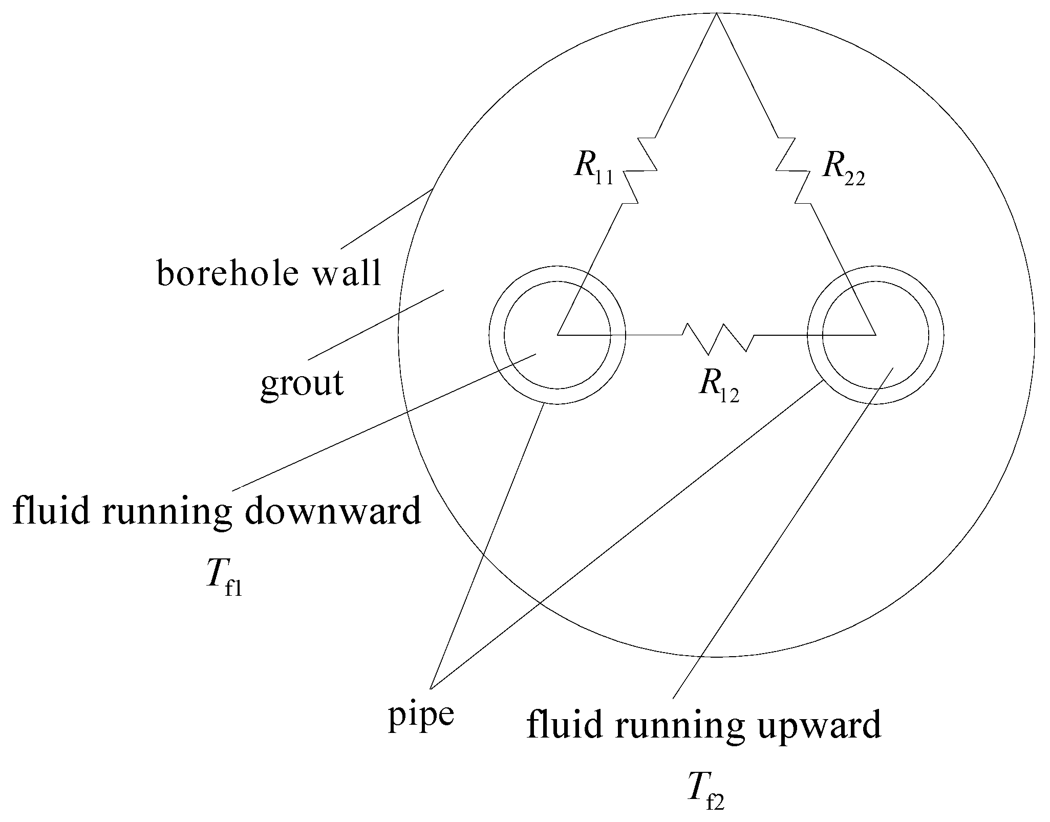
3.1. Heat Transfer Model inside the Boreholes

Zeng et al. [35] proposed a quasi-three-dimensional model, which takes into account the fluid axial convective heat transfer and the thermal “short-circuiting” among the U-tube legs. In addition, the conduction in the grout and ground is neglected in the axial direction, in order to simplify the model. The analytical solution for this model is as follows [35]:

$$\frac{T_{out}-T_b}{T_{in}-T_b}=\left[\cosh \left(\frac{H}{mc\sqrt{\left(R_{11}^2-R_{12}^2\right)}}\right)-\sqrt{\frac{R_{11}-R_{12}}{R_{11}+R_{12}}}\sinh \left(\frac{H}{mc\sqrt{R_{11}^2-R_{12}^2}}\right)\right]$$

(5)

where $T_{\text{b}}$ denotes the temperature of the borehole wall, $T_{\text{in}}$ and $T_{\text{out}}$ are the temperatures of the circulating water at the inlet and outlet, H is the borehole length, m is the mass flow rate of the circulating water, and c is the specific heat.

Furthermore, $R_{11}$ and $R_{22}$ in Equation (5) are the values of the thermal resistance between the circulating water and the borehole wall, and $R_{12}$ is the resistance between two individual pipes, as shown in Figure 1. They can be expressed as:

$$\{\begin{array}{l}{R}_{11}=R_{22}=\frac{1}{2\mathsf{\pi }{\mathsf{\lambda }}_g}\left(\ln \frac{r_b}{r_o}+\frac{{\mathsf{\lambda }}_g-{\mathsf{\lambda }}_s}{{\mathsf{\lambda }}_g+{\mathsf{\lambda }}_s}\ln \frac{4r_b^2}{4r_b^2-D^2}\right)+\frac{1}{2\mathsf{\pi }{\mathsf{\lambda }}_p}\ln \frac{r_b}{r_i}+\frac{1}{2\mathsf{\pi }{h}_i{r}_i}\\ R_{12}=\frac{1}{2\mathsf{\pi }{\mathsf{\lambda }}_g}\left(\ln \frac{r_b}{D}+\frac{{\mathsf{\lambda }}_g-{\mathsf{\lambda }}_s}{{\mathsf{\lambda }}_g+{\mathsf{\lambda }}_s}\ln \frac{4r_b^2}{4r_b^2+D^2}\right)\end{array}$$

(6)

where $r_{\text{i}}$ denotes the inner radius of the pipe, $r_{\text{o}}$ is the outer radius of the pipe, $r_{\text{b}}$ is the radius of the borehole, D is the spacing of U-tube shanks, and ${\mathsf{\lambda }}_{\text{g}}$, ${\mathsf{\lambda }}_{\text{p}}$, and ${\mathsf{\lambda }}_{\text{s}}$ denote the conductivity of the grout, pipe, and soil, respectively.

Figure 1. Thermal resistances in the borehole.

Figure 1. Thermal resistances in the borehole.

Also, in Equation (6) above, $h_{\text{i}}$ denotes the convective heat transfer coefficient of the circulating water, which can be calculated as follows [36]:

$$h_{\text{i}}=\frac{0.023{\mathrm{Re}}^{0.8}{\mathrm{Pr}}^{0.35}{\mathsf{\lambda }}_{\text{w}}}{2r_{\text{i}}}$$

(7)

where $\mathrm{Re}$ denotes the Reynolds number of the circulating water, and $\mathrm{Pr}$ is the Prandtl number.

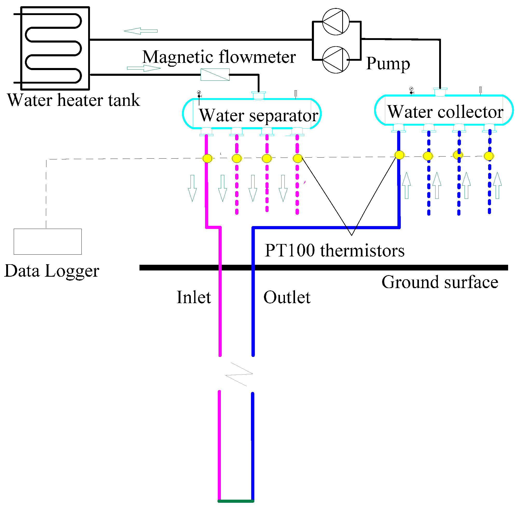
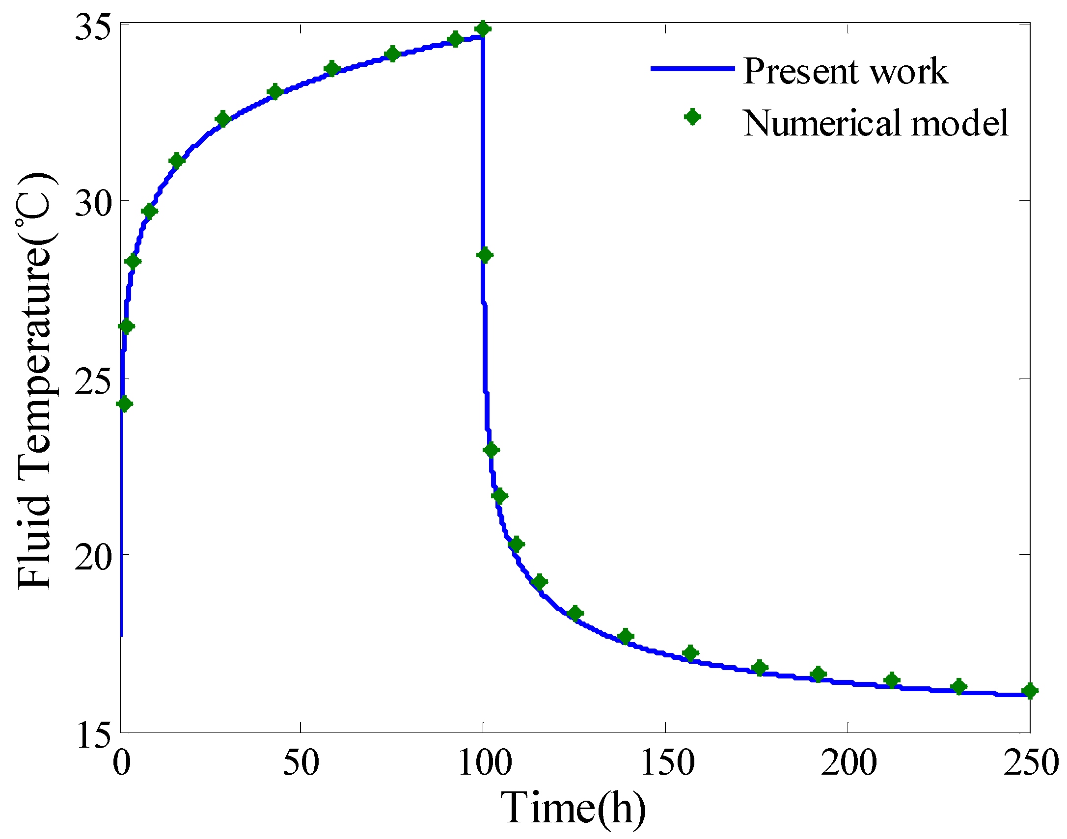
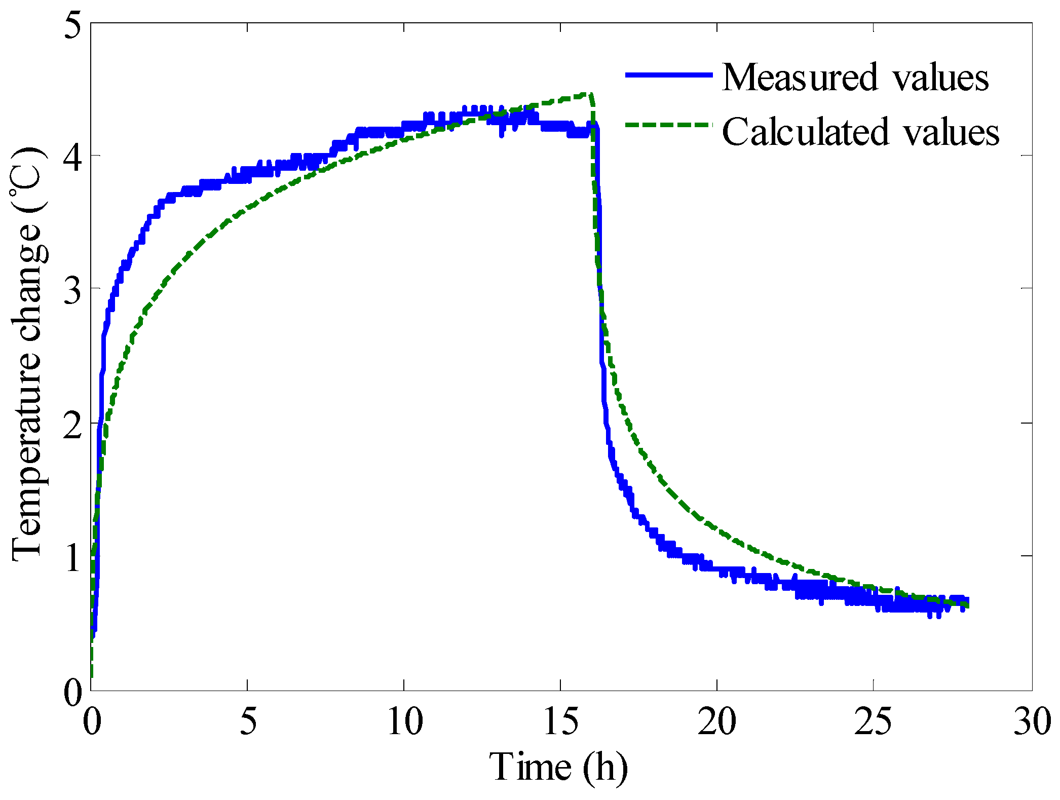
3.2. Experiment and Validation

In order to validate the accuracy of the model, an in situ test was done in Nanjing, China. The test system consisted of circulating heated water in a closed loop, a pump, BHEs, PT100 temperature sensors, a magnetic flow gauge, and other auxiliary devices. All sensors and the magnetic flow gauge were connected to a data acquisition system. The measurements were recorded every minute. The accuracy was calibrated before the experiment for all devices. The experiment was carried out with one BHE. During the test, the electric heater worked continuously for 16 h continuously. The water continued circulating inside the pipe for 12 h after the heating was stopped. The inlet and outlet water temperatures were recorded by the data acquisition system. The diagram of the system is shown in Figure 2. The parameters of the soil and the buried pipe are shown in Table 1.

Figure 2. Diagram of the test system.

Figure 2. Diagram of the test system.

Table 1. Parameters of the soil and borehole exchanger.

Item	Value
Borehole length, H	100 m
Borehole radius, rb	0.06 m
Internal pipe radius, ri	0.014 m
External pipe radius, ro	0.016 m
Thermal conductivity of pipe, λp	0.6 W·m−1·K−1
Thermal conductivity of soil, λs	2.13 W·m−1·K−1
Volumetric thermal capacity of soil, ρscs	1.76 × 106 J·m−3·K−1
Thermal conductivity of grout, λg	2.4 W·m−1·K−1
Thermal conductivity of water, λw	0.6 W·m−1·K−1
Volumetric thermal capacity of water, ρwcw	4.2 × 106 J·m−3·K−1
Fluid velocity inside pipe, u	0.4 m·s−1

Table 1. Parameters of the soil and borehole exchanger.

Item	Value
Borehole length, H	100 m
Borehole radius, rb	0.06 m
Internal pipe radius, ri	0.014 m
External pipe radius, ro	0.016 m
Thermal conductivity of pipe, λp	0.6 W·m−1·K−1
Thermal conductivity of soil, λs	2.13 W·m−1·K−1
Volumetric thermal capacity of soil, ρscs	1.76 × 106 J·m−3·K−1
Thermal conductivity of grout, λg	2.4 W·m−1·K−1
Thermal conductivity of water, λw	0.6 W·m−1·K−1
Volumetric thermal capacity of water, ρwcw	4.2 × 106 J·m−3·K−1
Fluid velocity inside pipe, u	0.4 m·s−1

Since it was unclear if there was groundwater flow in the experimental area, and what its flux was, that flux was set to 0 m·s⁻¹ when we calculated the temperature change of the circulating water at the outlet. The comparison of the calculated values with the experimental results is shown in Figure 3. There is good agreement between the two sets, which validates the model and confirms that it can be used with confidence in further research. Compared to the calculated values, the experimental measurements reach near-steady state more quickly. This may be due to the groundwater flow, which promotes the heat exchange of the BHE and accelerates the heat diffusion downstream. In addition, the groundwater flow leads to a faster recovery of the geo-temperature.

In order to verify the accuracy of the model in predicting the long-term operation and restoration process, the model was also validated with the numerical model presented by Ozudogru et al. [37]. A test was performed in a borehole with a single loop, by applying a constant heat rate of 50 W·m⁻¹ for the duration of 100 h. After loading, the temperatures were recorded for a recovery period of 150 h. The ground surface was kept at a constant temperature, equal to the undisturbed temperature, in both the model presented here and the numerical model from the literature. The input parameters used in our model and numerical analysis were the same as those in the literature.

Figure 3. Comparison of the calculated values with the experimental results.

Figure 3. Comparison of the calculated values with the experimental results.

Figure 4 shows a comparison between the mean fluid temperatures in the geothermal loops predicted in the present work and the numerical model. This figure shows that the results from the two models are in good agreement.

Figure 4. Comparison between the proposed model (solid line) and the numerical model.

Figure 4. Comparison between the proposed model (solid line) and the numerical model.

4. Results and Discussion

In order to evaluate the geo-temperature restoration performance, the geo-temperature recovery rate can be defined as:

$$\mathsf{\xi }=\frac{t\prime -t}{t_0-t}=\frac{\Delta t-\Delta t\prime }{\Delta t}$$

(8)

where all parameters characterize the soil—t₀ is the initial temperature, t is the temperature after the GSHP stops, t′ is the temperature after recovery, $\Delta t$ is the temperature change after the GSHP stops, and Δt′ is the temperature change after recovery.

4.1. Soil Temperature Recovery at Different Depths of the BHE

Calculations in heating mode were carried out in order to evaluate the geo-temperature recovery characteristics at different depths along the borehole. For this purpose, a single BHE was considered during five years of intermittent operation, which involved each year a sequence of four months in active mode and eight months in idle mode. The parameters of the soil and the BHE are shown in Table 1. The groundwater flux was set at 0 m/s, i.e., the groundwater flow was ignored.

Figure 5 shows the temperature changes around the borehole wall at depths of 0.25, 0.5, 0.75, 50, and 99 m. The figure shows that the geo-temperature changes are smaller at the two ends of the BHE, compared to temperature changes in the middle (at depth of 50 m), when considering the heat transfer along the borehole axis. For example, in the first cycle, when t = 120 d, the maximum temperature changes are 4.604, 6.194, 6.884, 10.11, and 8.842 °C at the five depths, respectively. The geo-temperature restoration rate has the opposite trend. For example, at the end of the cycle, for t = 360 days, the recovery rates are 0.9975, 0.9960, 0.9950, 0.9547, and 0.9715 at the five depths, the minimum being observed at a depth of 50 m. It can also be shown that, while the operation cycle is in progress, the maximum soil temperature change increases gradually, while the growth rate decreases. In that case the soil temperature recovery rate also decreases, with values of 0.9960, 0.9939, 0.9917, 0.9103, and 0.9431 at the end of the fifth operation cycle.

Figure 5. Temperature changes in different depths of the BHE.

Figure 5. Temperature changes in different depths of the BHE.

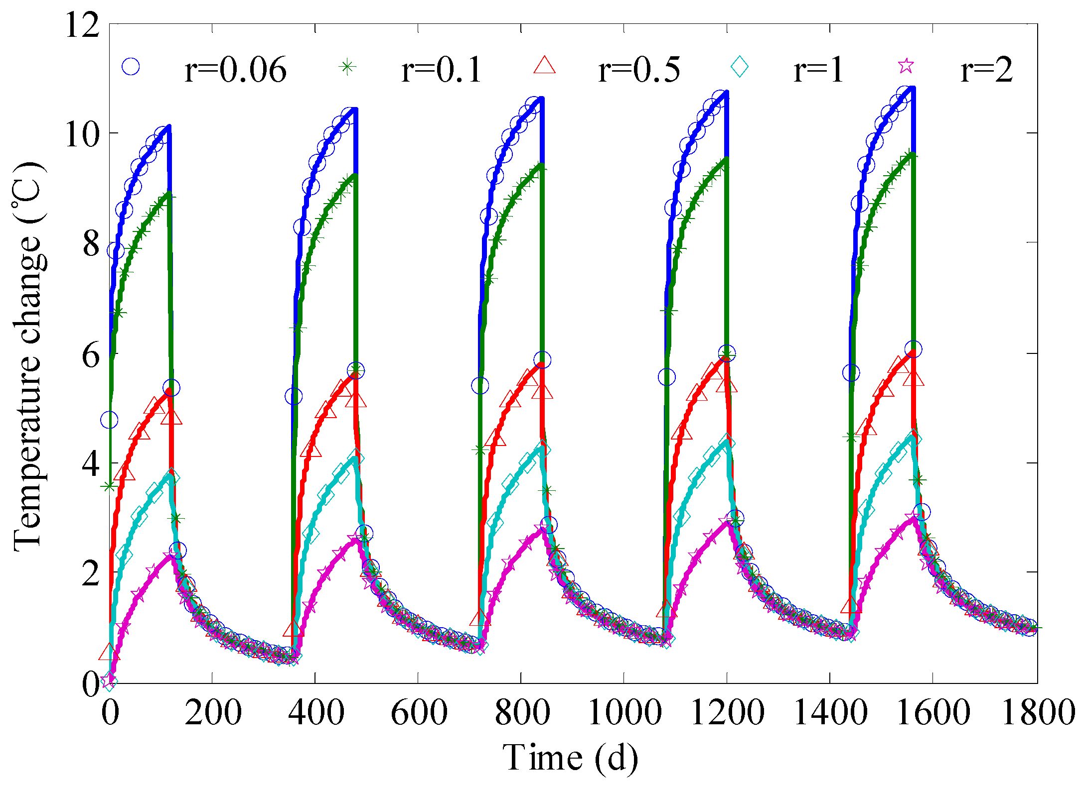
4.2. Geo-Temperature Recovery Characteristic at Different Distances from the BHE

Figure 6 shows the geo-temperature changes at different distances from the BHE, r = 0.06, 0.1, 0.5, 1, 2, and 4 m, for the same depth z = 50 m.The initial and boundary conditions are the same as those in Section 4.1. From Figure 6 it can be seen that, the closer to the borehole wall, the greater the amplitude variation of the soil temperature change, and the faster the soil temperature recovery. For example, at a distance of r = 0.06 m in the fifth operation cycle, after 240 d of geo-temperature recovery, the recovery rate is 0.9090. In contrast, at the larger distance of r = 2 m, the recovery rate is only 0.6830. In addition, it is also possible to establish that, due to the low thermal diffusivity of the soil, the time at which a maximum soil temperature is observed increases as the distance r increases.

In practice, depending on the size of the heat pump units and the ground properties, more than one BHE are used, with various geometrical configurations. After a long time of operation, the temperature variations at the various BHEs begin to interact. The soil temperature recovery process in such arrays of BHEs becomes more complex. For this reason, we further analyze the geo-temperature recovery characteristics of the BHE fields from four different aspects—BHE spacing, heat flow rate per unit length, operation strategy, and effect of the groundwater flow. To simplify the calculations, we use the example of an array with nine BHEs in a 3 × 3 grid (Figure 7).

Figure 6. Geo-temperature recovery at different distances from the BHE.

Figure 6. Geo-temperature recovery at different distances from the BHE.

Figure 7. 3 × 3 square layout of nine BHEs.

Figure 7. 3 × 3 square layout of nine BHEs.

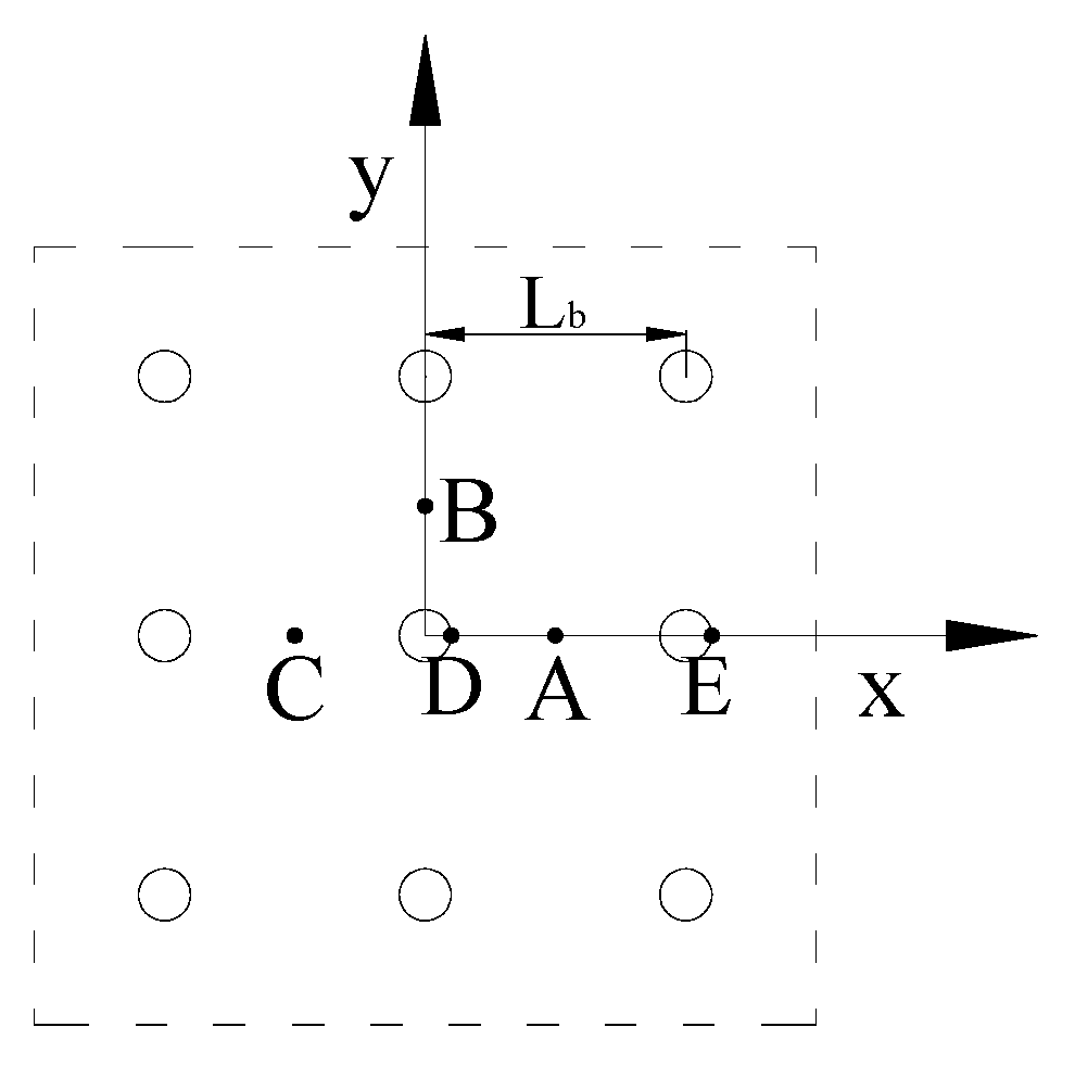
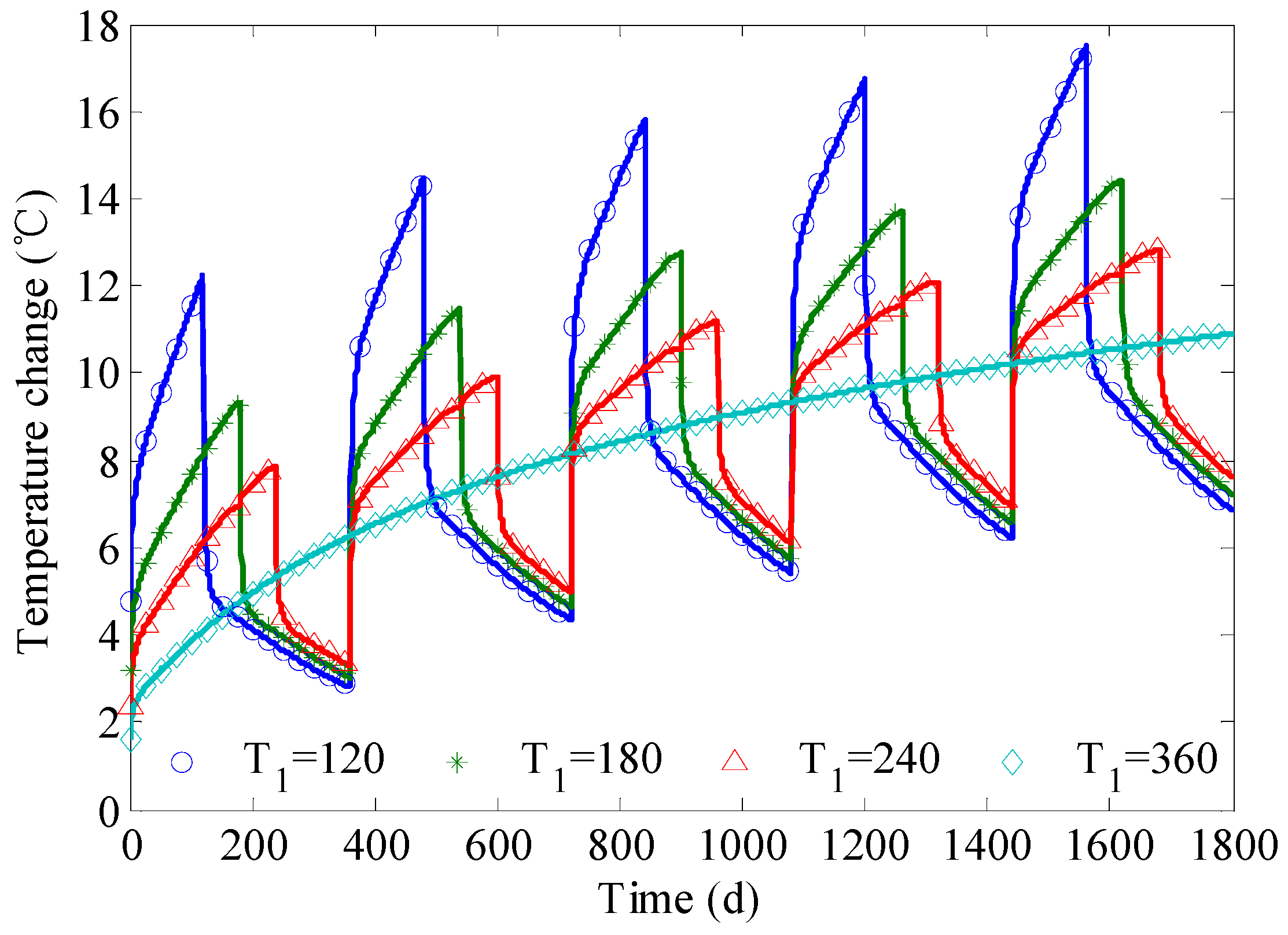
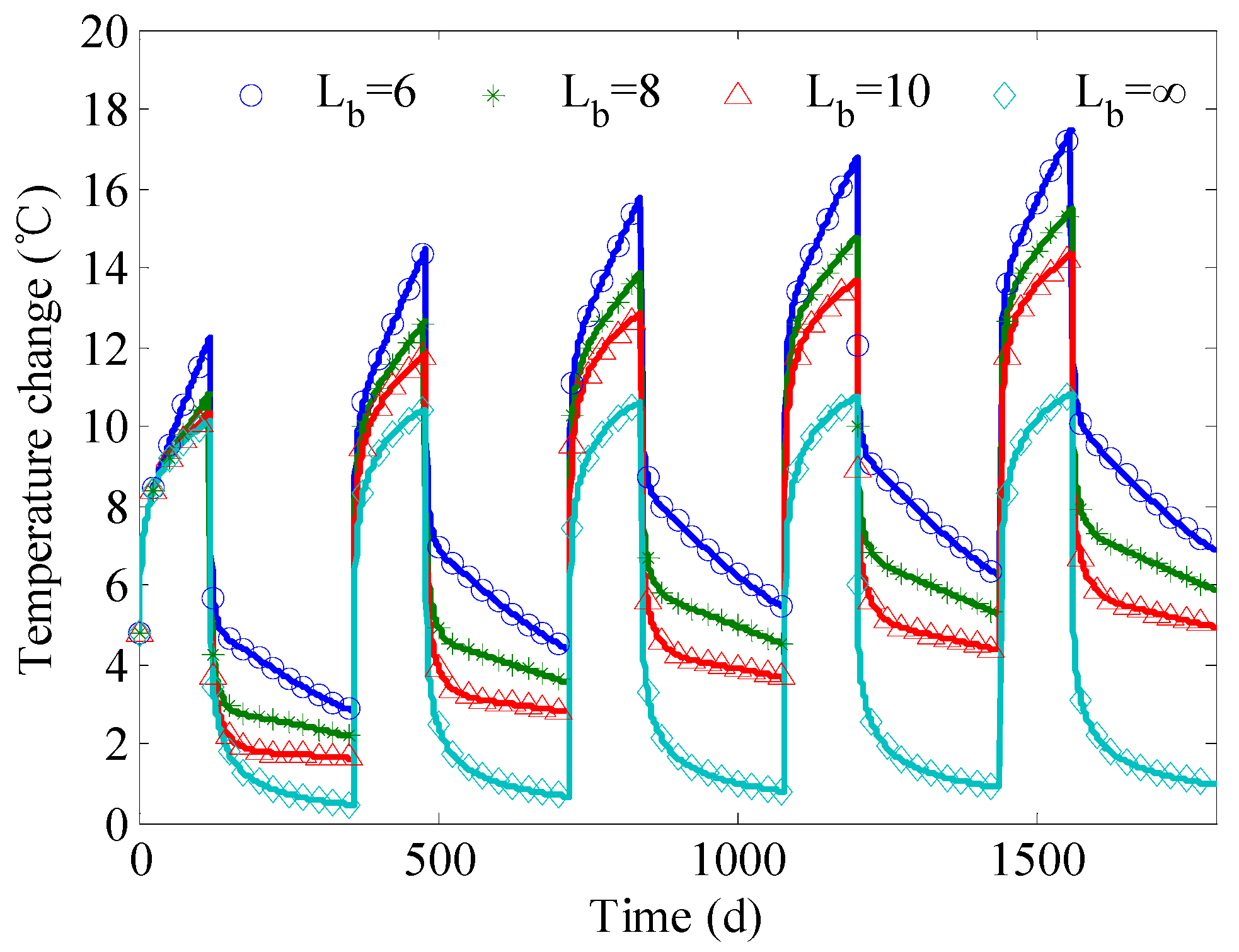
4.3. Effect of BHE Spacing

To explore the effect of BHE spacing on the soil temperature change and heat recovery rate, point D(0.06, 0) from Figure 7 is considered as an example, for inter pipe spacing of L_b = 6, L_b = 8, L_b = 10, and L_b = ∞ m. The calculations for L_b = ∞ are in fact for a single BHE, as the influence of the other BHEs can be ignored. The initial and boundary conditions are the same as in Section 4.1.

The soil temperature changes at a depth of 50 m for different values of the BHE spacing are presented in Figure 8. As the BHE spacing increases, the interference between the BHEs decreases, the maximum geo-temperature change also decreases, and the heat recovery gets better. Considering the fifth cycle as an example, the temperature change after recovery drops to 6.876, 5.878, 4.932, and 0.964 °C for the four different values of BHE spacing. The heat recovery rates in this case are 0.6069, 0.6200, 0.6556, and 0.9108. Therefore, for long-term sustainability of a multiple BHE system with an unbalanced thermal load, an adequate borehole separation distance is essential. This distance should be coordinated with the load and operation time of the BHE so as to avoid occupying too large of an area.

Figure 8. Soil temperature changes at point D for different values of the BHE spacing.

Figure 8. Soil temperature changes at point D for different values of the BHE spacing.

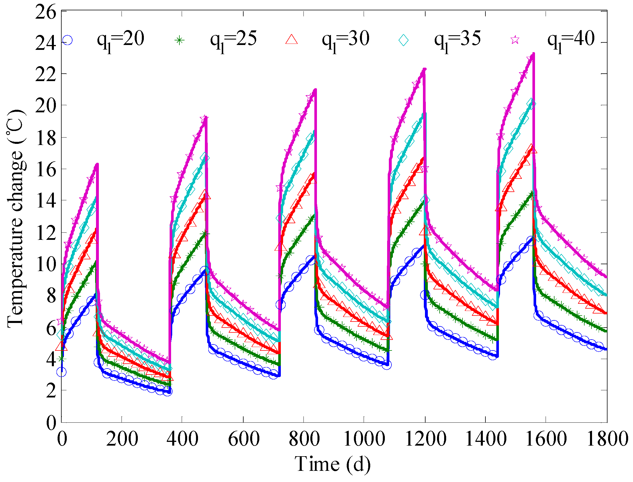
4.4. Effect of Heat Flow Rate per Unit Length

To analyze the influence of the heat flow rate on the geo-temperature change of the BHE fields, the temperature changes at point D(0.06, 0) are considered for five different heat flow rates per unit length: 20, 25, 30, 35, and 40 W·m⁻¹. The pipe spacing used is 6 m. The effect of ground water flow is ignored in this case. Initial and boundary conditions are same as before.

The calculated results are shown in Figure 9. At the end of the first cycle, the maximum temperature changes are 8.147, 10.18, 12.22, 14.26, and 16.29 °C, for the five values of the heat flow rates. The heat recovery rate is 0.7695 for all heat flow rates. At the end of the fifth cycle, the maximum temperature changes are 11.66, 14.57, 17.49, 20.4, and 23.32 °C, respectively, and the heat recovery rate is still a constant, but reduced by 19% to 0.6069, compared to the first cycle. It can then be concluded that the heat flow rate strongly influences the soil temperature change, but is inconsequential for the geo-temperature recovery rate. The heat recovery rate depends on the ground conditions, meteorological parameters, and some other factors.

Figure 9. Geo-temperature changes at point D for different heat flow rates.

Figure 9. Geo-temperature changes at point D for different heat flow rates.

4.5. Effect of the Operation Mode

Studies show that the operation model significantly affects the coefficient of performance (COP) of the GSHP system. When considering the influence of the operation mode, we must ensure that the heat discharged into the ground is the same for all operation modes, otherwise the comparison is meaningless. For this reason, this section discusses the analysis of the soil temperature changes at point D(0.06, 0) for five different operation modes. The operation times are 120, 180, 240, and 360 d. The corresponding heat flow rates per unit length are 30, 20, 15, and 10 W·m⁻¹.

Figure 10 shows the calculated results for the different operation modes, ignoring the influence of the ground water flow. This figure shows that the greater the heat flow rate, the greater the temperature change of the soil, and the faster the geo-temperature recovery. The reason is that the intermittent operation allows the soil enough time to recover, in contrast to a continuous operation with a low heat flow rate. In addition, excessively high heat flow rates lead to increased outlet temperatures, which impair the COP of the GSHP system. Therefore, when choosing the heat flow rate under intermittent operation, both the geo-temperature recovery and the COP of the GSHP must be taken into account.

Figure 10. Geo-temperature changes at point D for different operation modes.

Figure 10. Geo-temperature changes at point D for different operation modes.

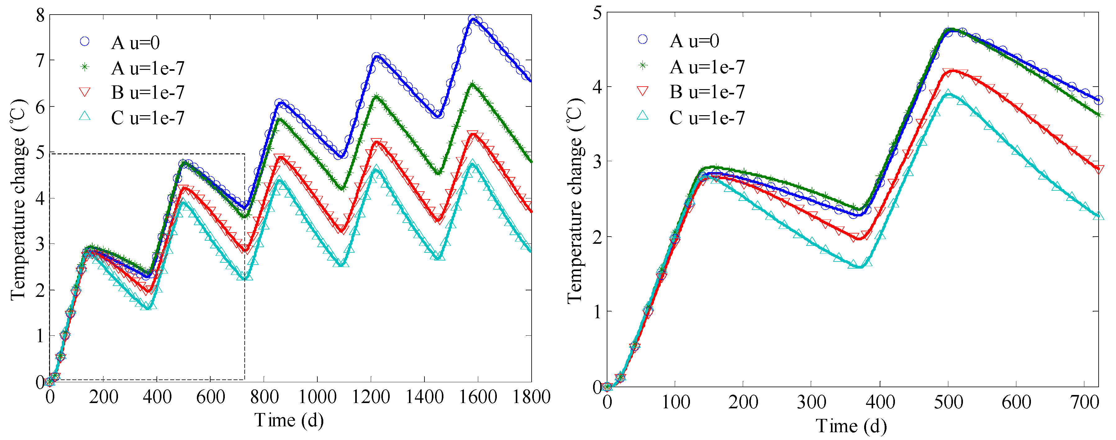
4.6. Effect of the Ground Water Flow on the Temperature Changes at Different Locations

In the case of multiple boreholes interacting with the groundwater flow, the interference between the BHEs becomes evident and the temperature changes vary at different locations of the array. In order to investigate the influence of the groundwater flow in this case, the temperature changes at three symmetrical points are analyzed—A(3, 0), B(0, 3), and C(−3, 0). In these calculations, we assume that the groundwater flux along the x axis is 1 e⁻⁷ m·s⁻¹, the heat flow rate per unit length is 30 W·m⁻¹, the soil porosity is 0.25, and the pipe spacing is 6 m.

The temperature changes at the three points are shown in Figure 11 for five different cycles. This figure shows that the temperature changes at point B and C increase at a smaller rate compared with the temperature change at point A because the groundwater flow accelerates the diffusion of heat downstream, rendering the geo-temperature change more complex. By comparing the temperature changes at point A in two cases, with and without groundwater flow, at the beginning of the operation, for t < 520 d, the soil temperature change is greater in the presence of groundwater flow, However for t > 520 d, the temperature change rapidly increases in the absence of groundwater flow. Therefore, in the case of a short-term operation, if the BHE fields are arranged improperly, it is possible that the groundwater flow causes damage to the running of downstream BHEs.

It is to be noted that in the case of a long-term operation, the groundwater flow accelerates the geo-temperature recovery process. As an example, in the fifth cycle, the geo-temperature recovery rates at point A with and without groundwater flow are 0.2599 and 0.1740, respectively.

Figure 11. Geo-temperature changes at different locations, considering groundwater flow.

Figure 11. Geo-temperature changes at different locations, considering groundwater flow.

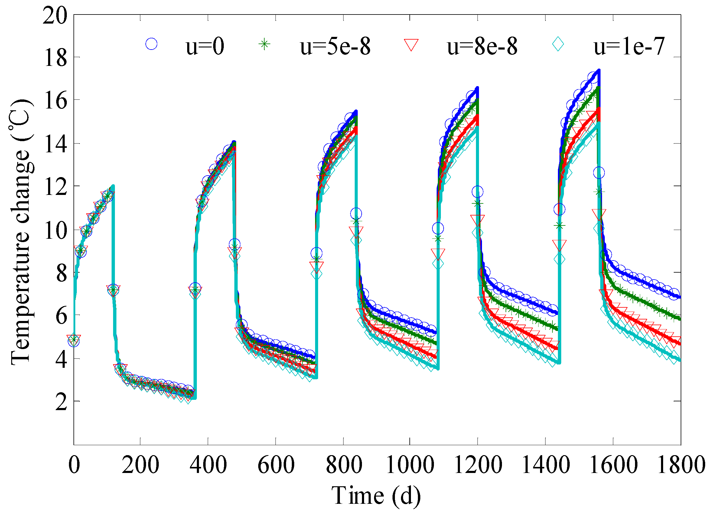
4.7. Effect of Groundwater Flux

Groundwater flux is influenced by the hydraulic gradient and the hydraulic conductivity coefficient. The differences between the hydrogeological conditions and soil properties in different regions can be significant, so that the groundwater flux is different from one place to another. In order to investigate its influence on the geo-temperature recovery rate, we calculate the temperature changes at the BHE fields for five different cycles, for four groundwater fluxes values—0 m·s⁻¹, 5 e⁻⁸ m·s⁻¹, 8 e⁻⁸ m·s⁻¹, and 1 e⁻⁷ m·s⁻¹. The parameters of the BHEs and the ground are the same as above.

The temperature changes at point D(0.06, 0) are shown in Figure 12. It can be seen that the greater the groundwater flux, the lower the temperature change and the better the soil heat recovery. For example, at the end of the fifth cycle, the temperature changes for the four different values of the groundwater flux are 6.827, 5.817, 4.66, and 3.906 °C. The corresponding heat recovery rates are 0.6076, 0.6494, 0.7011, and 0.7379, respectively.

Figure 12. Effect of the groundwater flux on the geo-temperature changes at point D.

Figure 12. Effect of the groundwater flux on the geo-temperature changes at point D.

5. Conclusions

In this work we establish the analytical solution for analyzing the geo-temperature restoration performance of the BHE fields, considering the effect of groundwater flow. This is achieved by combining the moving finite line source model with the g-function and the superposition principle. The factors influencing the geo-temperature recovery in the BHE fields are also analyzed. The conclusions of this work are as follows:

(1)

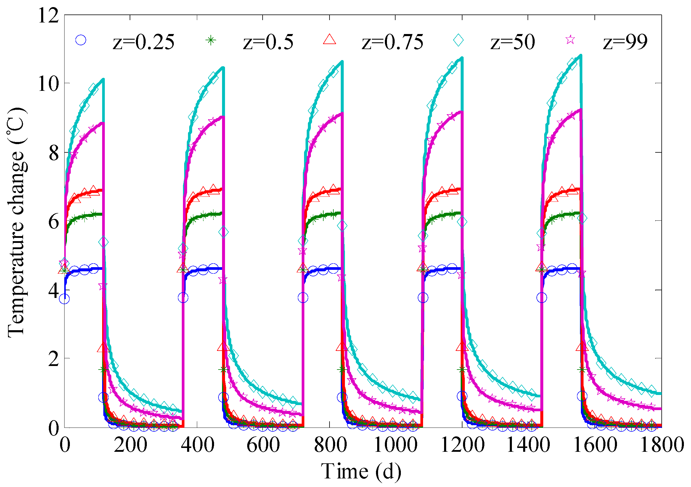
Due to the influence of the ground surface and the heat transfer along the borehole, the geo-temperature changes are smaller at the two ends of the BHE compared to the change in the middle. The heat transfer along the borehole significantly influences the geo-temperature restoration rate. Therefore, in the case of long-term operations, the axial effect should be taken into account.

(2)

Closer to the borehole wall, the amplitude variations of the soil temperature change are greater and the geo-temperature recovery is better.

(3)

With the increase of BHE spacing, the thermal interference between the BHEs decreases, the maximum soil temperature change is reduced, and the heat recovery improves. Thus, for long-term sustainability of a multiple BHE system with an unbalanced load, adequate borehole separation distance is essential.

(4)

The heat flow rate significantly influences the soil temperature change, but has no effect on the geo-temperature recovery rate. This rate only depends on the ground conditions, meteorological parameters, and other factors.

(5)

Compared to continuous operation with a low load, intermittent operation with a higher load performs better.

(6)

Groundwater flow accelerates the diffusion of heat to downstream. Therefore, if the BHE fields are arranged improperly, the groundwater flow can cause damage to the running of downstream BHE. For a long-term operation, the groundwater flow is beneficial to the geo-temperature recovery process even for downstream BHEs.

(7)

For a given point in the BHE fields, the greater the groundwater flux, the lower the temperature change and the better the geo-temperature recovery.

References

1. Capozza, A.; de Carli, M.; Zarrella, A. Design of borehole heat exchangers for ground-source heat pumps: A literature review, methodology comparison and analysis on the penalty temperature. Energy Build. 2012, 55, 369–379. [Google Scholar] [CrossRef]
2. Koohi-Fayegh, S.; Rosen, M.A. On thermally interacting multiple boreholes with variable heating strength: Comparison between analytical and numerical approaches. Sustainability 2012, 4, 1848–1866. [Google Scholar] [CrossRef]
3. Yang, H.; Cui, P.; Fang, Z. Vertical-borehole ground-coupled heat pumps: A review of models and systems. Appl. Energy 2010, 87, 16–27. [Google Scholar] [CrossRef]
4. Yuan, Y.; Cao, X.; Sun, L.; Lei, B.; Yu, N. Ground source heat pump system: A review of simulation in China. Renew. Sustain. Energy Rev. 2012, 16, 6814–6822. [Google Scholar] [CrossRef]
5. Li, S.; Yang, W.; Zhang, X. Soil temperature distribution around a U-tube heat exchanger in a multi-function ground source heat pump system. Appl. Therm. Eng. 2009, 29, 3679–3686. [Google Scholar] [CrossRef]
6. Gao, J.; Zhang, X.; Liu, J.; Li, K.S.; Yang, J. Thermal performance and ground temperature of vertical pile-foundation heat exchangers: A case study. Appl. Therm. Eng. 2008, 28, 2295–2304. [Google Scholar] [CrossRef]
7. Qian, H.; Wang, Y. Modeling the interactions between the performance of ground source heat pumps and soil temperature variations. Energy Sustain. Dev. 2014, 23, 115–121. [Google Scholar] [CrossRef]
8. Yang, W.; Chen, Y.; Shi, M.; Spitler, J.D. Numerical investigation on the underground thermal imbalance of ground-coupled heat pump operated in cooling-dominated district. Appl. Therm. Eng. 2013, 58, 626–637. [Google Scholar] [CrossRef]
9. ASHRAE. Commercial/Institutional Ground-Source Heat Pump Engineering Manual; American Society of Heating, Refrigerating and Air-Conditioning Engineerings Inc.: Atlanta, GA, USA, 1995. [Google Scholar]
10. Yavuzturk, C.; Spitler, J.D. Comparative study of operating and control strategies for hybrid ground-source heat pump systems using a short time step simulation model. Ashrae Trans. 2000, 106, 192–209. [Google Scholar]
11. Sayyadi, H.; Nejatolahi, M. Thermodynamic and thermoeconomic optimization of a cooling tower-assisted ground source heat pump. Geothermics 2011, 40, 221–232. [Google Scholar] [CrossRef]
12. Qi, Z.; Gao, Q.; Liu, Y.; Yan, Y.Y.; Spitler, J.D. Status and development of hybrid energy systems from hybrid ground source heat pump in China and other countries. Renew. Sustain. Energy Rev. 2014, 29, 37–51. [Google Scholar] [CrossRef]
13. Cao, X.; Yuan, Y.; Sun, L.; Lei, B.; Yu, N.; Yang, X. Restoration performance of vertical ground heat exchanger with various intermittent ratios. Geothermics 2015, 54, 115–121. [Google Scholar] [CrossRef]
14. Ingersoll, L.R.; Plass, H.J. Theory of the ground pipe heat source for the heat pump. ASHVE Trans. 1948, 47, 339–348. [Google Scholar]
15. Bernier, M.A. Ground-coupled heat pump system simulation. Ashrae Trans. 2001, 107, 605–616. [Google Scholar]
16. Michopoulos, Α.; Κyriakis, Ν. Predicting the fluid temperature at the exit of the vertical ground heat exchangers. Appl. Energy 2009, 86, 2065–2070. [Google Scholar] [CrossRef]
17. Lee, C.K. Effects of multiple ground layers on thermal response test analysis and ground-source heat pump simulation. Appl. Energy 2011, 88, 4405–4410. [Google Scholar] [CrossRef]
18. Yavuzturk, C.; Spitler, J.D.; Rees, S.J. A transient two-dimensional finite volume model for the simulation of vertical U-tube ground heat exchangers. ASHRAE Trans. 1999, 105, 465–474. [Google Scholar]
19. Javed, S.; Fahlén, P.; Claesson, J. Vertical ground heat exchangers: A review of heat flow models. In Proceedings of the Effstock 2009, Stockholm, Sweden, 14–17 June 2009.
20. Cui, P.; Yang, H.; Fang, Z. Numerical analysis and experimental validation of heat transfer in ground heat exchangers in alternative operation modes. Energy Build. 2008, 40, 1060–1066. [Google Scholar] [CrossRef]
21. Gao, Q.; Li, M.; Yu, M. Experiment and simulation of temperature characteristics of intermittently-controlled ground heat exchanges. Renew. Energy 2010, 35, 1169–1174. [Google Scholar] [CrossRef]
22. Shang, Y.; Li, S.; Li, H. Analysis of geo-temperature recovery under intermittent operation of ground-source heat pump. Energy Build. 2011, 43, 935–943. [Google Scholar] [CrossRef]
23. Signorelli, S. Geoscientific Investigations for the Use of Shallow Low-Enthalpy Systems. Ph.D. Thesis, Swiss Federal Institute of Technology Zürich, Zürich, Switzerland, 2004. [Google Scholar]
24. Lazzari, S.; Priarone, A.; Zanchini, E. Long-term performance of BHE (borehole heat exchanger) fields with negligible groundwater movement. Energy 2010, 35, 4966–4974. [Google Scholar] [CrossRef]
25. Zanchini, E.; Lazzari, S.; Priarone, A. Long-term performance of large borehole heat exchanger fields with unbalanced seasonal loads and groundwater flow. Energy 2012, 38, 66–77. [Google Scholar] [CrossRef]
26. Dehkordi, S.E.; Schincariol, R.A. Effect of thermal-hydrogeological and borehole heat exchanger properties on performance and impact of vertical closed-loop geothermal heat pump systems. Hydrogeol. J. 2013, 22, 189–203. [Google Scholar] [CrossRef]
27. Erol, S.; Hashemi, M.A.; François, B. Analytical solution of discontinuous heat extraction for sustainability and recovery aspects of borehole heat exchangers. Int. J. Therm. Sci. 2015, 88, 47–58. [Google Scholar] [CrossRef]
28. Lamarche, L.; Beauchamp, B. A new contribution to the finite line-source model for geothermal boreholes. Energy Build. 2007, 39, 188–198. [Google Scholar] [CrossRef]
29. Molina-Giraldo, N.; Bayer, P.; Blum, P. Evaluating the influence of thermal dispersion on temperature plumes from geothermal systems using analytical solutions. Int. J. Therm. Sci. 2011, 50, 1223–1231. [Google Scholar] [CrossRef]
30. Lous, M.L.; Larroque, F.; Dupuy, A.; Moignard, A. Thermal performance of a deviated deep borehole heat exchanger: Insights from a synthetic coupled heat and flow model. Geothermics 2015, 57, 157–172. [Google Scholar] [CrossRef]
31. Molina-Giraldo, N.; Blum, P.; Zhu, K.; Bayer, P.; Fang, Z. A moving finite line source model to simulate borehole heat exchangers with groundwater advection. Int. J. Therm. Sci. 2011, 50, 2506–2513. [Google Scholar] [CrossRef]
32. Eskilson, P. Thermal Analysis of Heat Extraction Boreholes. Ph.D. Thesis, University of Lund, Lund, Sweden, 1987. [Google Scholar]
33. Hellstrom, G. Ground Heat Storage, Thermal Analysis of Duct Storage Systems. Ph.D. Thesis, Department of Mathematical Physics, University of Lund, Sweden, 1991. [Google Scholar]
34. Diao, N.R.; Fang, Z.H. Ground-Coupled Heat Pump Technology; Higher Education Press: Beijing, China, 2006. (In Chinese) [Google Scholar]
35. Zeng, H.; Diao, N.; Fang, Z. Heat transfer analysis of boreholes in vertical ground heat exchangers. Int. J. Heat Mass Transf. 2003, 46, 4467–4481. [Google Scholar] [CrossRef]
36. Bergman, T.L.; Incropera, F.P.; Lavine, A.S. Fundamentals of Heat and Mass Transfer; John Wiley & Sons: Hoboken, NJ, USA, 2011. [Google Scholar]
37. Ozudogru, T.Y.; Olgun, C.G.; Senol, A. 3d numerical modeling of vertical geothermal heat exchangers. Geothermics 2014, 51, 312–324. [Google Scholar] [CrossRef]