Comparative Influences of Precipitation and River Stage on Groundwater Levels in Near-River Areas

Abstract

The sustainable performance of foundations of various urban buildings and infrastructures is strongly affected by groundwater level (GWL), as GWL causes changes in the stress state within soil. In the present study, the components affecting GWL were investigated, focusing on the effects of precipitation and river stage. These components were analyzed using a six-year database established for hydrological and groundwater monitoring data. Five study regions for which daily measured precipitation, river stage, and GWL data were available were compared. Different periods of precipitation, geographical characteristics, and local surface conditions were considered in the analysis. The results indicated that key influence components on GWL are different depending on the hydrological, geological, and geographical characteristics of the target regions. River stage had the strongest influence on GWL in urban areas near large rivers with a high ratio of paved surface. In rural areas, where the paved surface area ratio and soil permeability were low, the moving average showed a closer correlation to GWL than river stage. A moving average-based method to predict GWL variation with time was proposed for regions with a low ratio of paved surface area and low permeability soils.

1. Introduction

Load-carrying capability and deformation are key design components of various buildings and infrastructures to ensure the proper level of serviceability during the lifetime of the structures. These design components are strongly affected by the stress state within soil, which varies with groundwater level (GWL), resulting in changes in soil effective stress and pore water pressure [1]. Although there are no apparent indications of failure or collapse conditions, changes in GWL can cause a considerable amount of ground subsidence and instant instability problems, all of which are related to the functionality and performance of target structures [2,3]. Various investigations into the effects of GWL on the performance of foundation structures have been performed, and design methods to take GWL into account have been proposed [4,5,6,7]. The results from these investigations indicated that incorporation of GWL into the design is essential to guarantee the sustainable performance of structures and to prevent unexpected damage during the lifetime of the structures due to additional settlement or reductions in bearing capacity.

GWL varies and fluctuates for various reasons, including uneven annual precipitation and changes in river stage. Other components that affect GWL variation are the duration and intensity of preceding precipitation, proximity to the river, and pumping and recharge activities [8,9,10,11]. Moving average, which is the cumulative precipitation during a certain past period, was introduced as a more refined expression for precipitation and better captures the characteristics of GWL and its variations than precipitation [8,9]. Guttmann [9] and Murray [12] both used the moving average and showed that the moving average is closely related to the variation in GWL over time. Winter [13], Sanders [14], and Kelly [15], by contrast, reported that river stage had the greatest effect on variations in GWL.

Most previous studies of GWL have focused on individual and uncoupled influences of hydrological components, such as precipitation, accumulated rainfall, and river stage as well as regional pumping and recharging activities. However, the effects of these components can differ depending on the geographic and geomorphic characteristics of target areas, such as proximity to rivers, soil profiles, and ground surface conditions. In particular, because most urban and residential areas are located near rivers, comparative analyses that address the effects of various components that can influence GWL are required, as there may be some reciprocal effects among influencing components.

In the present study, significant influence components on GWL and its variation are investigated, focusing on the effects of precipitation and river stage. These components were analyzed using a multi-year database of hydrological and GWL monitoring data and compared among five study regions for which daily measured precipitation, river stage level, and GWL fluctuations data were available. Different time scales of precipitation, geographical characteristics, and local surface conditions were considered. A method for GWL estimation is proposed based on the moving average for regions with a low paved surface area ratio and low permeability soils.

2. Study Regions and Data Descriptions

2.1. Study Regions

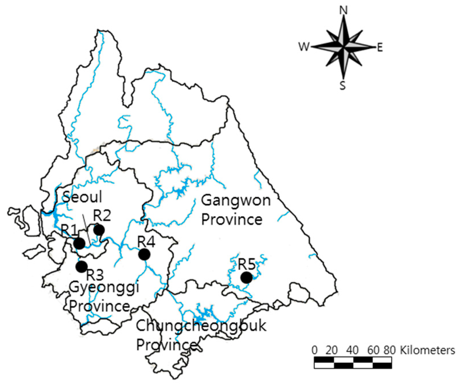
Five regions were selected and introduced to analyze the comparative effects of various influencing components on GWL and its variations (Figure 1). The five regions were located in different areas near Seoul, Gyeonggi, and Gangwon provinces in Korea, with different soil types and geographical conditions. These selected regions are referred to as regions R1–R5 in this paper. Based on the geographical characteristics of these areas, target study regions were categorized into three groups: group A (R1), group B (R2 and R3), and group C (R4 and R5). Group A represents locations near a large river and urban areas where surface conditions are mostly impermeable due to a high paved surface area ratio (higher than 97%). Regions in group B are also urban areas with paved surface area ratios higher than 90%. Compared to group A, regions in group B are located near smaller-sized rivers with lower paved surface area ratios. Regions R4 and R5 in group C represent rural areas with paved surface area ratios lower than 35%.

Figure 1. Locations of study regions.

Figure 1. Locations of study regions.

The locations of regions R1–R5 are shown in Figure 1. Region R1 is located near the Han River, one of the largest rivers in Korea. The distance of the GWL observatory in region R1 from the Han River is 156 m. Regions R2 and R3 are located near Ui and Anyang streams at distances of 253 and 203 m from rivers, respectively. The geographical and hydrological characteristics of each region are shown in Table 1. Detailed hydrological and size information about the rivers listed in Table 1 is provided in Table 2.

Table 1. Geographical and precipitation characteristics of study regions.

Region	Group	Nearby River	Paved Area Ratio (%)	Mean Annual Precipitation (mm)	Distance (m)
R1	A	Han River	97.4	1344	156
R2	B	Ui Stream	93.7	1344	253
R3	B	Anyang Stream	91.0	1451	203
R4	C	Namhan River	16.9	1294	431
R5	C	Dong River	32.0	1242	281

Table 1. Geographical and precipitation characteristics of study regions.

Region	Group	Nearby River	Paved Area Ratio (%)	Mean Annual Precipitation (mm)	Distance (m)
R1	A	Han River	97.4	1344	156
R2	B	Ui Stream	93.7	1344	253
R3	B	Anyang Stream	91.0	1451	203
R4	C	Namhan River	16.9	1294	431
R5	C	Dong River	32.0	1242	281

Table 2. Basic characteristics of the rivers in the five study regions.

River	Mean Width (m)	Basin Length (km)	Drainage Area (km2)	Normal Water Flow (m3/s)	Mean Discharge during Flood Season (m3/s)
Han River	1155	494	26,018	423	2456
Ui Stream	60	8	27	-	-
Anyang Stream	200	33	281	6	16
Namhan River	309	375	12,514	89	471
Dong River	242	65	2448	17	138

Table 2. Basic characteristics of the rivers in the five study regions.

River	Mean Width (m)	Basin Length (km)	Drainage Area (km2)	Normal Water Flow (m3/s)	Mean Discharge during Flood Season (m3/s)
Han River	1155	494	26,018	423	2456
Ui Stream	60	8	27	-	-
Anyang Stream	200	33	281	6	16
Namhan River	309	375	12,514	89	471
Dong River	242	65	2448	17	138

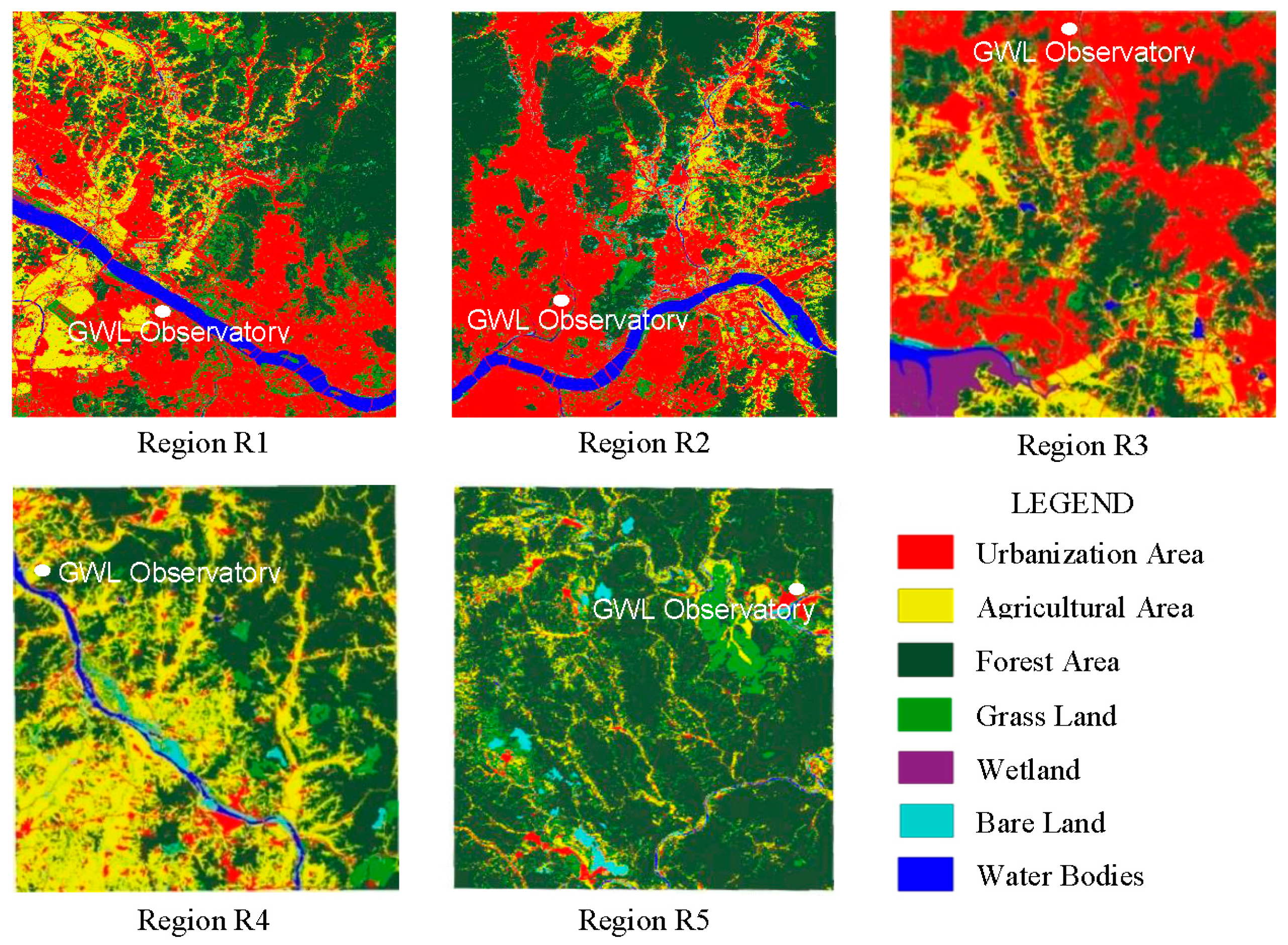
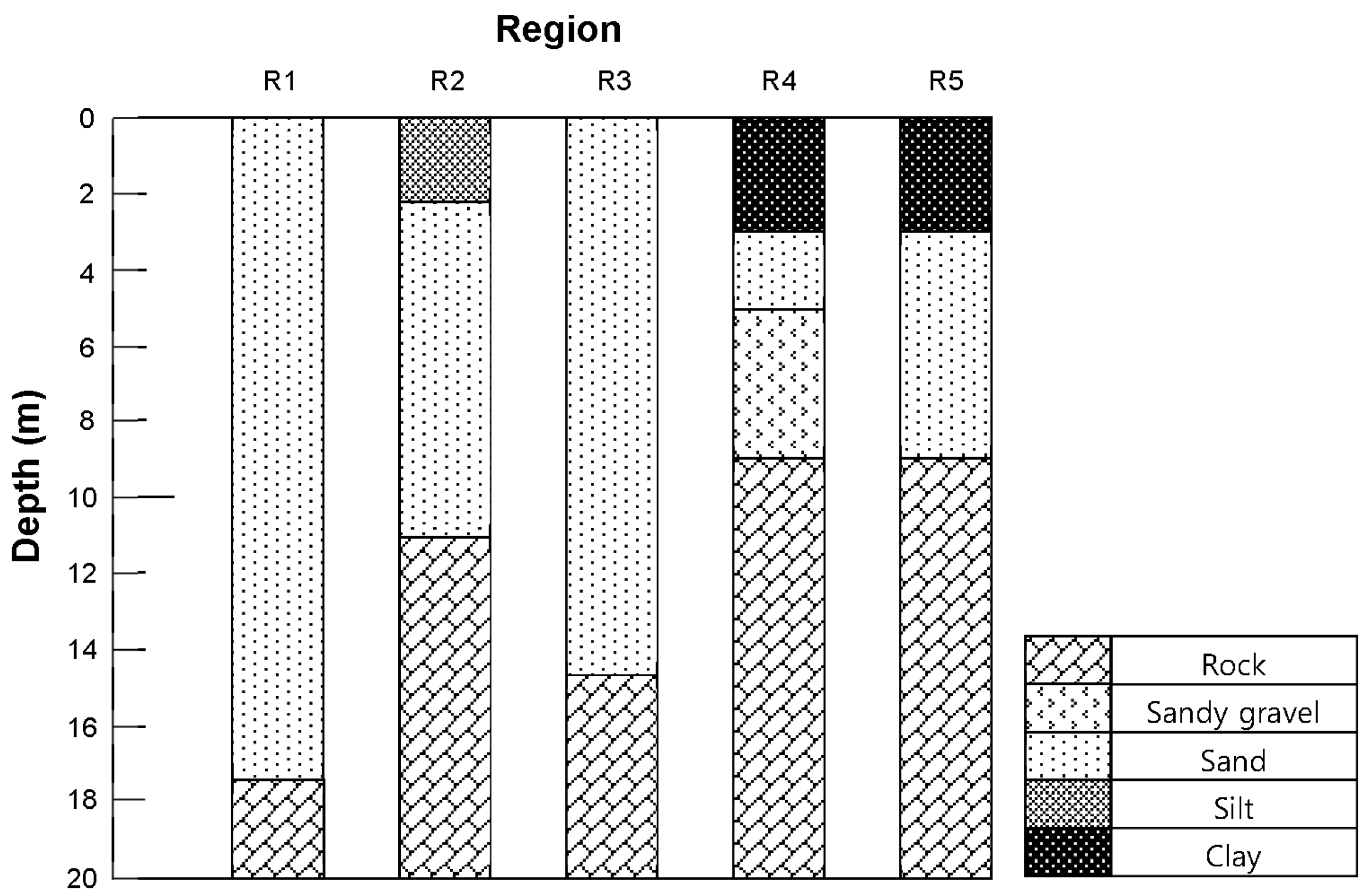
The land maps of all study regions, obtained from the Korean Ministry of the Environment, are shown and compared in Figure 2 [16]. The portions of paved surface areas in regions R1–R3 were higher than in regions R4 and R5 (Table 1). Soil profiles at the regions are indicated in Figure 3. Surface soils of regions R1–R3 were composed mainly of highly permeable granular soils, whereas the top soils of regions R4 and R5 (in rural areas) were composed of low permeability clays.

Figure 2. Surface conditions in study regions.

Figure 2. Surface conditions in study regions.

Figure 3. Soil profiles in the five study regions.

Figure 3. Soil profiles in the five study regions.

2.2. Precipitation, River Stages, and Groundwater Levels

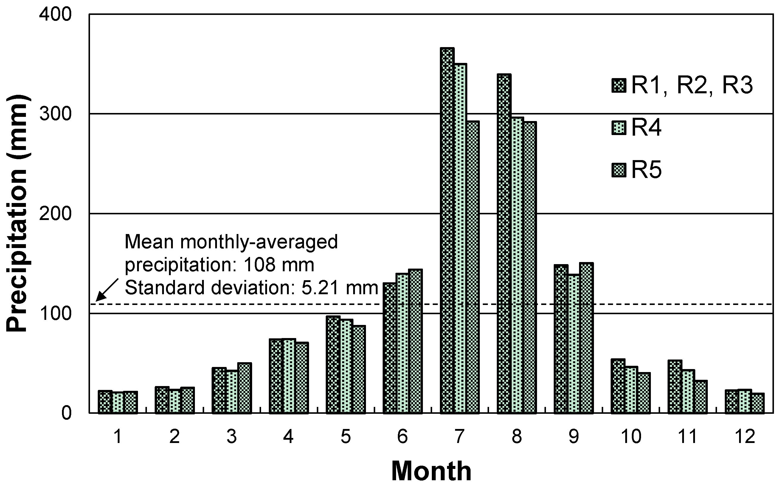
Typical patterns of annual precipitation in the study regions showed seasonally dependent variation with highly concentrated rainfall from July to August. Figure 4 shows the annual distributions of monthly averaged precipitation in regions R1–R4 during the past 37 years (1965 to 2001) [17] and in R5 during the past 30 years from 1981 to 2010 [18]. The amount of precipitation during July and August was noticeably high, more than twice the mean monthly-averaged precipitation.

Figure 4. Annual distributions of monthly averaged precipitation.

Figure 4. Annual distributions of monthly averaged precipitation.

A six-year database of precipitation, river stages, and GWL was established for the study regions and used in the correlation analysis. River stage and precipitation data were obtained from the Han River Flood Control Office [19], and GWL data were obtained from the National Groundwater Information and Service Center [20], both official organizations for flood and GWL control in Korea.

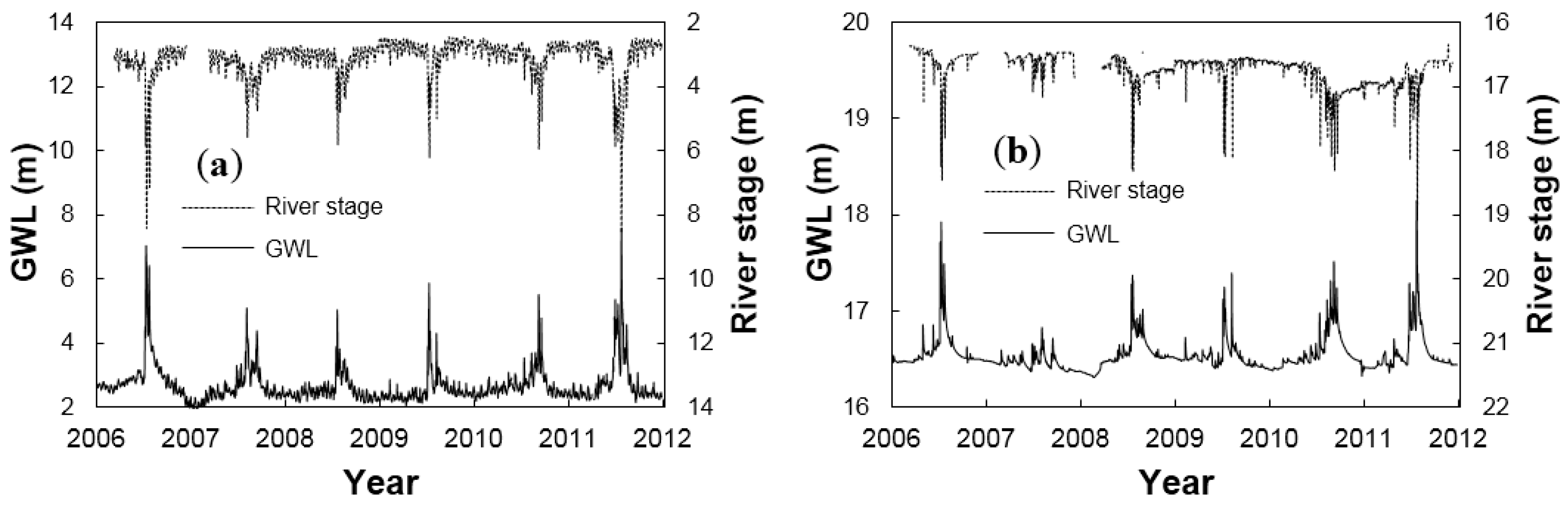
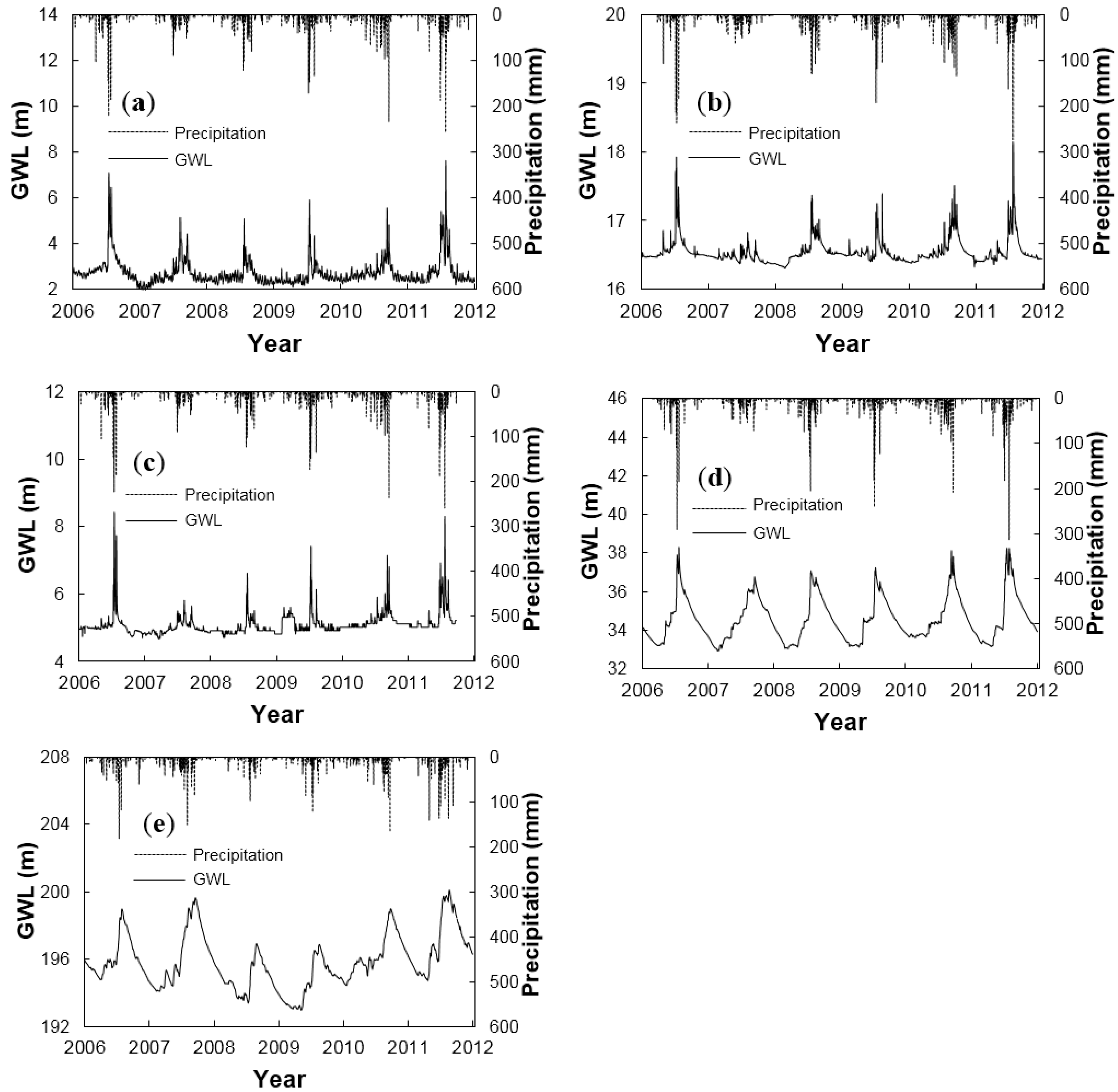
Figure 5 and Figure 6 show periodic variations of daily measured GWL for the six years from 2006 to 2011, plotted together with daily measured precipitation (Figure 5) and river stage (Figure 6). For region R5, river stage data were collected for four years due to a newly established observation facility in 2008. Note that the daily measured data were introduced because the safety margin of structures can also be affected by instant changes in stress and soil conditions. Similar patterns were observed each year with regard to summer-concentrated annual precipitation, river stage, and GWL. During the six-year monitoring period, the maximum annual fluctuation in GWL was 5.44 m in region R1. For regions R2 and R3 of group B, the maximum GWL fluctuations were 3.30 and 1.84 m, respectively. For R4 and R5 of group C, the maximum GWL fluctuations were 5.07 and 5.38 m, respectively. Detailed hydrological data for each region are summarized in Table 3.

Figure 5. Variations in GWL and precipitation for regions (a) R1; (b) R2; (c) R3; (d) R4; and (e) R5.

Figure 5. Variations in GWL and precipitation for regions (a) R1; (b) R2; (c) R3; (d) R4; and (e) R5.

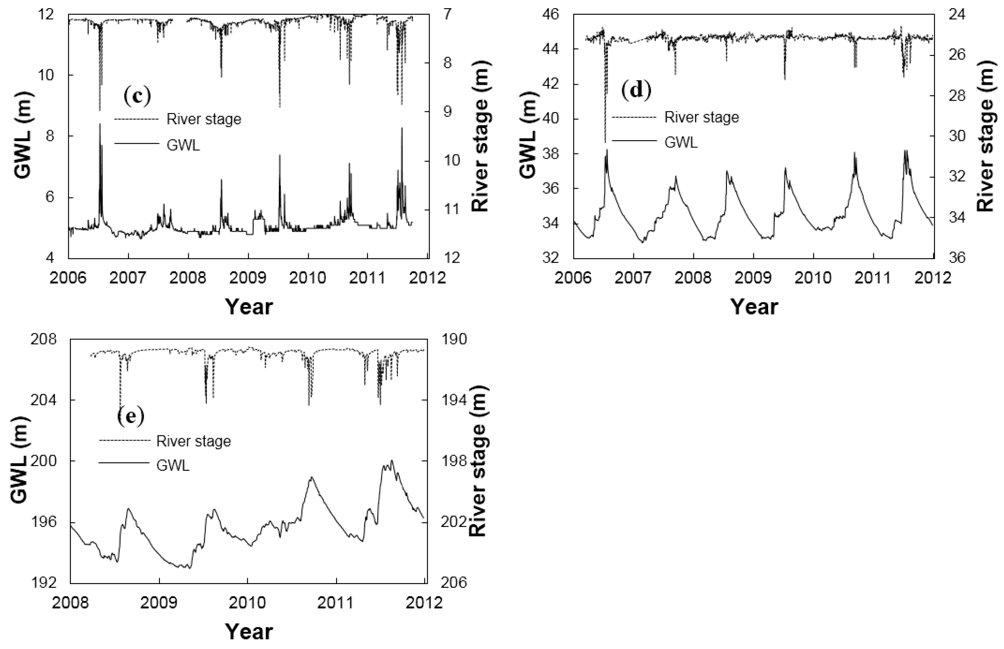
Figure 6. Variations in GWL and river stage for regions (a) R1; (b) R2; (c) R3; (d) R4; and (e) R5.

Figure 6. Variations in GWL and river stage for regions (a) R1; (b) R2; (c) R3; (d) R4; and (e) R5.

Table 3. Precipitation and river stage characteristics of the five study regions.

Region	Precipitation (mm)		River Stage (m)		GWL (m)
	Max. Level	Daily Mean	Peak Level	Mean Level	Max. Level	Mean Level
R1	237.0	4.0	8.6	3.1	7.6	2.7
R2	273.0	4.9	19.1	16.8	18.1	16.5
R3	258.0	4.0	9.0	7.1	8.4	5.1
R4	314.0	4.3	30.3	25.2	38.3	34.6
R5	181.0	3.8	195.5	190.5	200.1	194.7

Table 3. Precipitation and river stage characteristics of the five study regions.

Region	Precipitation (mm)		River Stage (m)		GWL (m)
	Max. Level	Daily Mean	Peak Level	Mean Level	Max. Level	Mean Level
R1	237.0	4.0	8.6	3.1	7.6	2.7
R2	273.0	4.9	19.1	16.8	18.1	16.5
R3	258.0	4.0	9.0	7.1	8.4	5.1
R4	314.0	4.3	30.3	25.2	38.3	34.6
R5	181.0	3.8	195.5	190.5	200.1	194.7

3. Methods for Data Analysis

3.1. Simple and Cross-Correlation Analyses

In the present study, simple and cross-correlation analyses, which are frequently adopted to check the validity of data correlation, were introduced for analyzing the influence levels of precipitation and river stage on GWL [21,22,23]. Cross-correlation analysis provides the degree of correlation, periodicity, and time lag between two sets of time-series data as expressed by the following equations:

$$r_{xy}(k)=\frac{C_{xy}(k)}{{\sigma }_x{\sigma }_y}$$

(1)

$$C_{xy}(k)=\frac{1}{n}{\displaystyle \sum _{i=1}^{n-k}(x_t-\overline{X})(y_{t+k}-\overline{Y})},$$

(2)

where x_t and y_t are time series data; $\overline{X}$ and $\overline{Y}$ are averages of x_t and y_t, respectively; σ_x and σ_y are standard deviations of x_t and y_t, respectively; k is the time lag; and n is the length of the time series. The best coefficient of correlation obtained from the cross correlation analysis was used for comparative analysis between two sets of time-series data. The results from the cross-correlation analyses were examined using t-tests to confirm statistical significance with respect to the time-series data.

3.2. Moving Average (MA) and Auto Regressive Moving Average (ARMA)

To further investigate the correlation between precipitation and GWL, a moving average was adopted, representing the average accumulated precipitation for a certain past period. Similar to other precipitation parameters, the moving average had minimum values close to zero during drought seasons and peak values during flood seasons. The moving average was originally introduced to estimate the drought index [9,11] and later applied to calculate the management index for groundwater dams and to consider the cumulative characteristics of preceding precipitation [24,25].

Because the moving average represents the accumulated amount of precipitation, it is determined through an iterative process. The iterative process involves calculating an average precipitation value over a certain past period of time that corresponds to the period when the best correlation to the target variable is achieved. Therefore, the moving average calculations should be repeated by increasing the number of periods examined until the best correlation is obtained. The auto regressive moving average (ARMA) is an improved method that assigns a certain weighted value to each past day from auto regressive analysis [26,27]. To evaluate the correlation of precipitation to GWL, the moving average and ARMA are used and compared.

4. Results

4.1. Precipitation

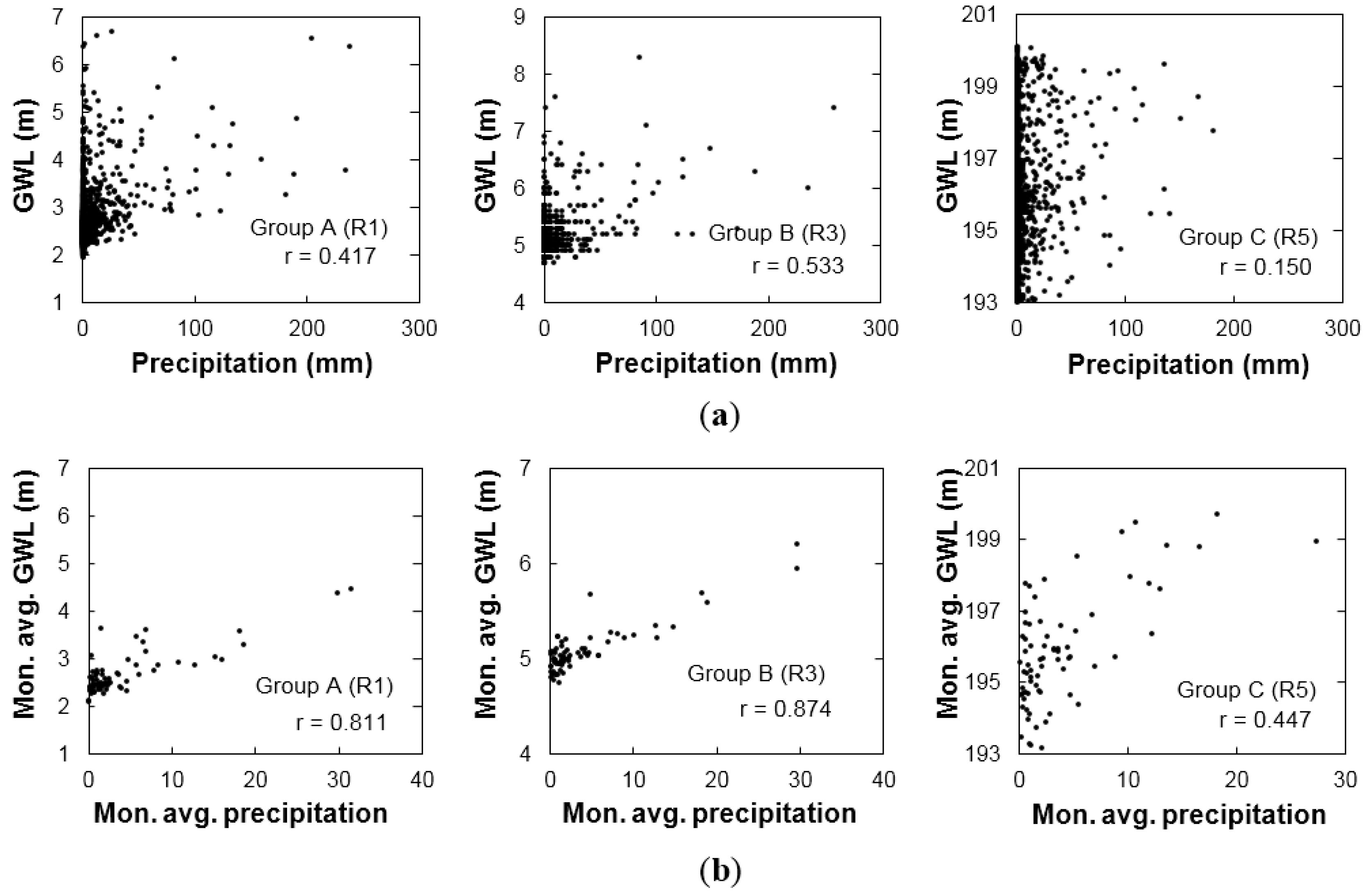
The average annual precipitation in Korea over the past 30 years was 1308 mm, nearly twice the world average. Because of the summer-concentrated characteristics of annual precipitation and time delays for rainfall infiltration into the ground, the timescale or resolution of the annual precipitation distribution can affect correlations to GWL. To analyze the effect of precipitation on GWL at different timescales, daily measured and monthly averaged precipitations were correlated to GWL. These are plotted in Figure 7a,b for regions R1, R3, and R5 of groups A, B, and C, respectively. The values of r (coefficient of correlation) for the match between GWL and precipitation data are indicated in Figure 7 and Table 4.

Figure 7. Comparison of GWL with (a) daily measured and (b) monthly averaged precipitations.

Figure 7. Comparison of GWL with (a) daily measured and (b) monthly averaged precipitations.

Table 4. Coefficients of correlation of components influencing GWL.

Region	Coefficient of Correlation (r)
	River Stage (Days) a	Daily Measured Precipitation (Days) a	Monthly Averaged Precipitation	Moving Average (Days) b	ARMA (Days) c
R1	0.931 (0)	0.417 (−1)	0.811	0.781 (10)	0.790 (22)
R2	0.605 (0)	0.349 (−1)	0.866	0.841 (19)	0.842 (38)
R3	0.676 (−1)	0.533 (−1)	0.874	0.798 (8)	0.789 (15)
R4	0.354 (−1)	0.293 (−13)	0.581	0.863 (81)	0.796 (58)
R5	0.453 (−11)	0.150 (−34)	0.447	0.875 (109)	0.732 (73)

^a Time lag from cross correlation analysis; ^b period for moving average; ^c period for ARMA.

Table 4. Coefficients of correlation of components influencing GWL.

Region	Coefficient of Correlation (r)
	River Stage (Days) a	Daily Measured Precipitation (Days) a	Monthly Averaged Precipitation	Moving Average (Days) b	ARMA (Days) c
R1	0.931 (0)	0.417 (−1)	0.811	0.781 (10)	0.790 (22)
R2	0.605 (0)	0.349 (−1)	0.866	0.841 (19)	0.842 (38)
R3	0.676 (−1)	0.533 (−1)	0.874	0.798 (8)	0.789 (15)
R4	0.354 (−1)	0.293 (−13)	0.581	0.863 (81)	0.796 (58)
R5	0.453 (−11)	0.150 (−34)	0.447	0.875 (109)	0.732 (73)

^a Time lag from cross correlation analysis; ^b period for moving average; ^c period for ARMA.

Figure 7a shows that there was no meaningful, unique correlation between daily measured precipitation and GWL, although the overall distribution of daily measured precipitation and GWL were similar, with both showing similar summer-concentrated patterns (Figure 5). Improved correlations were observed when monthly averaged GWL and precipitation were used (Figure 7b). This indicates that the GWL–precipitation correlation may change depending on the time resolution adopted, which in fact reflects the effect of preceding precipitation.

4.2. Moving Average

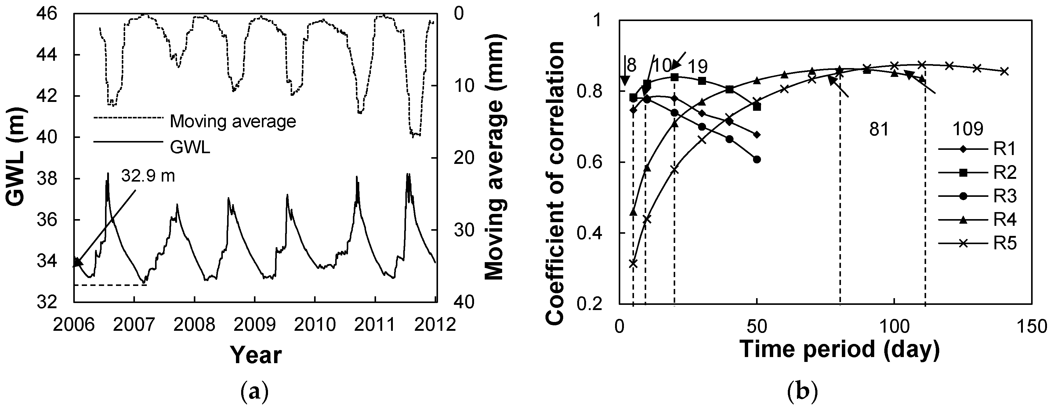
Each region considered in this study had different moving average periods that yielded the best correlation to GWL. Figure 8a,b show the correlation of the moving average to GWL for region R4 and the values of r as a function of period adopted to calculate the moving average for the study regions. The 32.9 m marked in Figure 8a is the minimum GWL that is necessary for the method proposed in this study, as will be explained later. The values of the moving average period for each region are indicated in Figure 8b. For regions R1–R3 of groups A and B, the moving average periods were 8, 10, and 19 days, respectively, while longer periods of 81 and 109 days were required for regions R4 and R5 of group C.

Figure 8. Correlation of moving average with GWL: (a) moving average and GWL with time and (b) coefficient of correlation with moving average period.

Figure 8. Correlation of moving average with GWL: (a) moving average and GWL with time and (b) coefficient of correlation with moving average period.

The difference in moving average periods shown in Figure 8b can be attributed to differences in soil type and permeability conditions, reflecting local, regional geological, and geographical conditions. As observed in Figure 3, regions in groups A and B had granular fill layers with high permeability near the top surface. For regions R4 and R5 of group C, fine-grained soil layers with a low permeability (k) of 1.66 × 10⁻³ cm/s and 2.46 × 10⁻⁴ cm/s, respectively, were present [20]. This suggests that the moving average period is strongly affected by the permeability of the soil, as soil permeability results in differences in how long it takes for rainfall to infiltrate into the ground and to contribute to GWL.

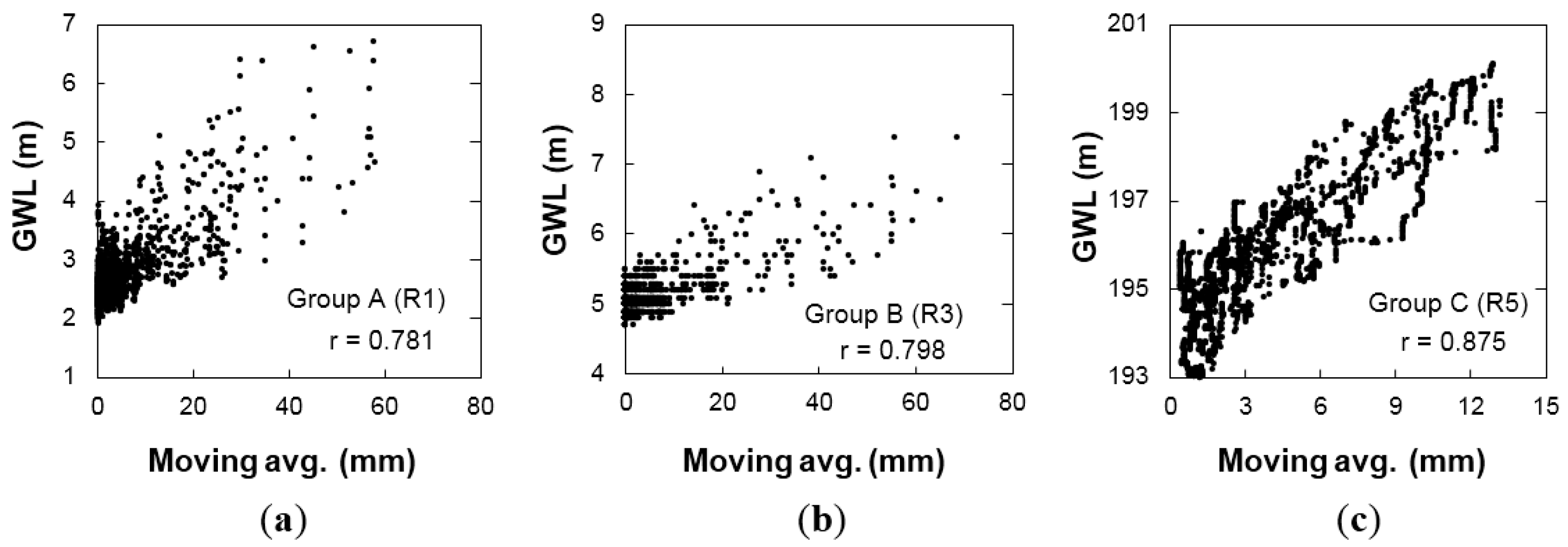
All GWL and moving average data for regions R1, R3, and R5 of groups A, B, and C are plotted in Figure 9. A higher correlation (higher r value) was observed for region R5 of group C while the lowest r value was obtained for region R1 of group A. A more detailed explanation and discussion of these results is provided in a Section 5.1.

Figure 9. Correlation between GWL and moving average for regions (a) R1; (b) R3; and (c) R5.

Figure 9. Correlation between GWL and moving average for regions (a) R1; (b) R3; and (c) R5.

4.3. River Stage

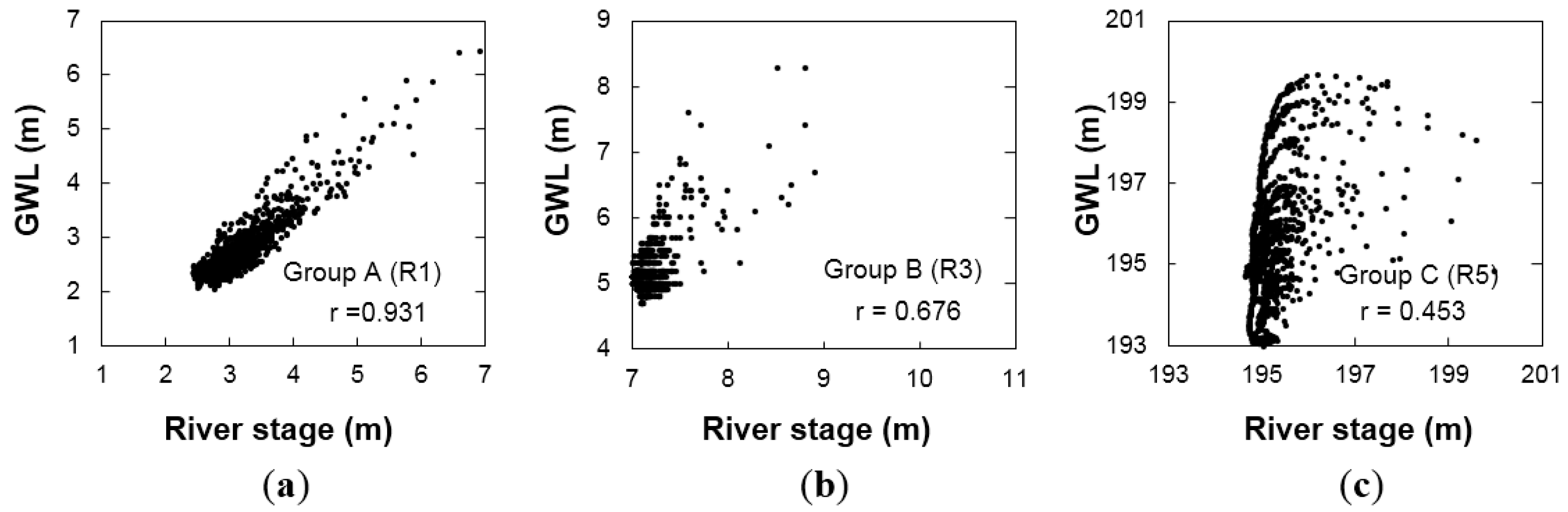
River stage is another component that can significantly influence GWL, particularly in areas near rivers. Measured GWL and river stage data for regions R1, R3, and R5 of groups A, B, and C were correlated (Figure 10). The values of r shown in Figure 10 for each region are summarized in Table 4. The best correlation between GWL and river stage was obtained for region R1 of group A (r = 0.931). For regions R4 and R5 of group C, r values were lower at 0.354 and 0.453, respectively.

Figure 10. Comparison of GWL and river stage for regions (a) R1; (b) R3; and (c) R5.

Figure 10. Comparison of GWL and river stage for regions (a) R1; (b) R3; and (c) R5.

4.4. Cross-Correlation Analysis Results

To examine the correlations of the various components with GWL in a more systematic manner, cross-correlation analysis was performed. Figure 11 shows results from the cross-correlation analysis of regions R1, R3, and R5 with river stage and the moving average that was best correlated to GWL for each region. Periodical characteristics of the correlations revealed that GWL, river stage, and precipitation all fluctuated with a certain annual periodicity. For regions R1 and R3, the cross-correlation was rougher with a time lag compared to that of region R5, which showed smoother variation. The cross-correlation values were close to unity for all cases at time lags equal to zero, confirming that the correlations among the components influencing GWL were sufficiently close.

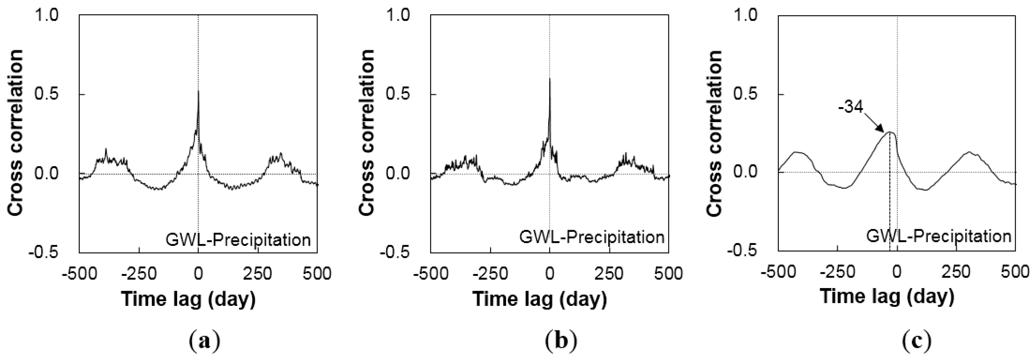
Figure 12 shows the results of a cross-correlation analysis between GWL and precipitation. Region R5 of group C showed a 34-day time lag for the correlation due to the time delay for rainfall infiltration, while regions R1 and R3 of groups A and B had no time lag. ARMA values are reported in Table 4. Longer ARMA periods were observed in regions in group C, consistent with the results shown in Figure 12.

Figure 11. Cross correlation results for regions (a) R1; (b) R3; and (c) R5.

Figure 11. Cross correlation results for regions (a) R1; (b) R3; and (c) R5.

Figure 12. Cross-correlation analysis results between GWL and precipitation for (a) R1; (b) R3; and (c) R5.

Figure 12. Cross-correlation analysis results between GWL and precipitation for (a) R1; (b) R3; and (c) R5.

5. Discussion and Proposed Method

5.1. Discussion

For all study regions, the period of peak GWL coincided with those of peak precipitation and river stage, while the patterns of GWL variation differed. GWL in groups A and B fluctuated within short time periods in a similar manner to variation in river stage. GWL in group C took a longer time to rise and fall, and showed smoother patterns of variation. Furthermore, GWL in Groups A and B showed rough fluctuation patterns that were very similar to the patterns observed for river stage variation.

The correlations between GWL and river stage, daily measured and monthly averaged precipitation, moving average, and ARMA are shown in Table 4. Note that the values in parentheses in each column are the time lags or periods that yielded the best correlation to GWL. The correlation to daily measured precipitation showed the lowest range of r values, while the correlations to moving average were higher overall with values of r higher than 0.78. This indicates that accumulated precipitation, which indicates the effect of preceding precipitation, is well correlated to GWL and thus more useful for the characterization of GWL. Time lags or periods for the correlation to the moving average of the study regions were different because of different soil and local surface conditions that resulted in different time delays for the impact of precipitation on GWL.

The correlation with river stage was strongly affected by the geographic condition of the target region. For region R1 in group A, which was located near a large river with a high paved surface area ratio, GWL was better correlated with river stage than daily measured or monthly averaged precipitation and the moving average. For regions R4 and R5 of group C, the correlations of GWL to the moving average were tighter than to river stage. For regions R2 and R3 of group B, the correlations of moving average and river stage to GWL were similar. Note that the ratios of paved surface area for both regions were above 91%, which is much higher than for regions R4 and R5 of group C.

The shape of the variation in GWL (see Figure 5 and Figure 6) is another issue to be addressed with regard to soil profile and soil permeability. As indicated in Figure 3, soils in regions R1–R3 consisted mainly of highly permeable sands, whereas regions R4 and R5 had low permeability clay layers near surfaces. For the regions in group C, as precipitation infiltrated vertically through the clay layers, the response period to GWL fluctuation became longer and the crumpled shapes of GWL were attenuated. For regions in groups A and B, river water, including runoff from precipitation, infiltrated horizontally through the highly permeable sand layers because of the large paved surface areas in these regions. Consequently, GWLs in regions in groups A and B were characterized by a pattern of rapid rise and fall as well as a crumpled shape. This suggests a correlation between the time period used to obtain the moving average and the permeability of the soil, and requires additional investigation.

5.2. Proposed GWL Correlation to Moving Average

5.2.1. Description of Methodology

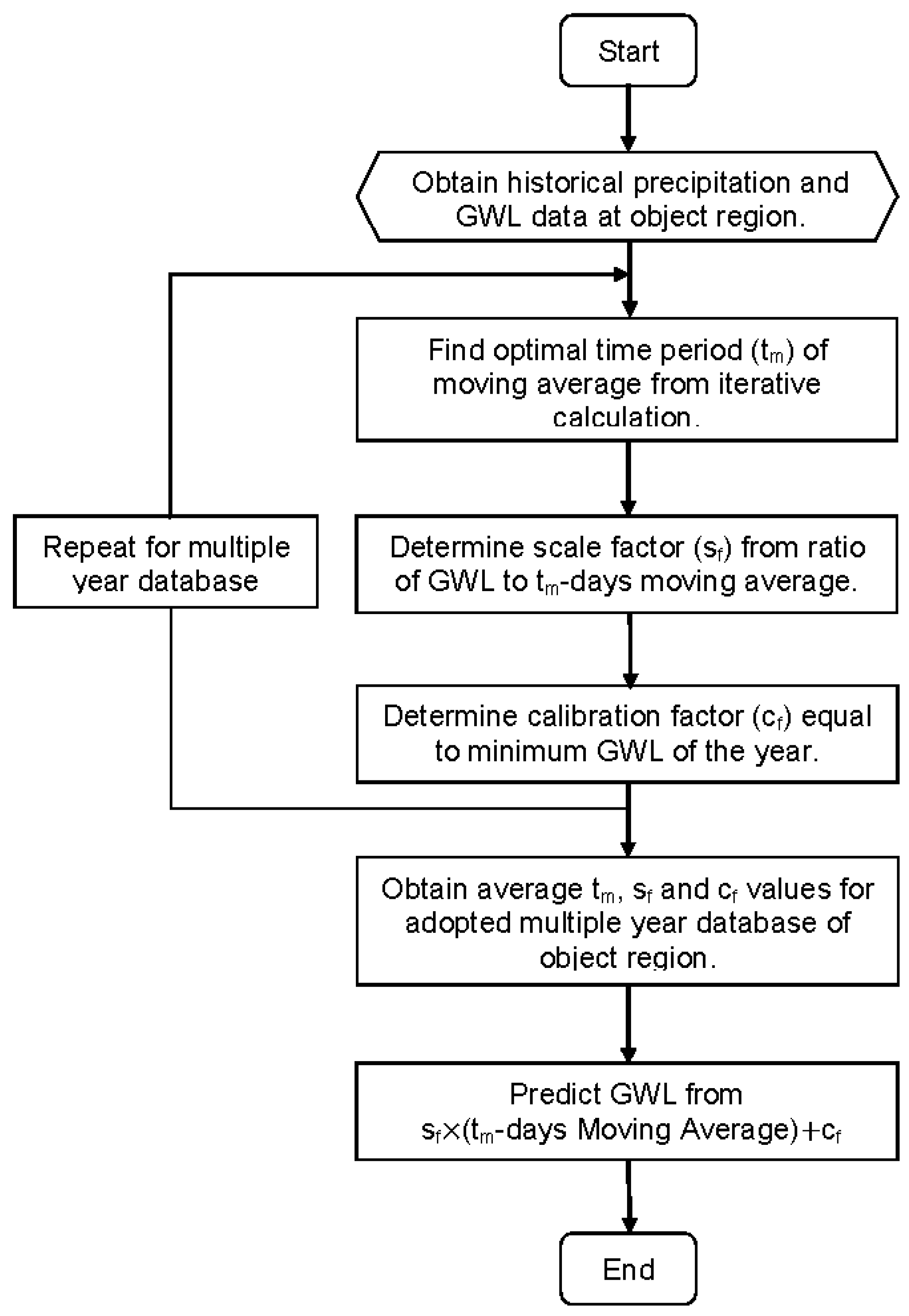
One important finding obtained in this study was that GWL is closely related to the moving average for areas with low permeability soils and a low paved surface area ratio. However, a close correlation between moving average and GWL itself does not guarantee accurate estimation of GWL, because the moving average period that gives the best correlation varies depending on local geological and geographical conditions. In this study, a more systematic yet simpler procedure for the estimation of GWL directly based moving average is explored and proposed. Adjustment and calibrating processes were introduced to better match the annual distribution of GWL and the moving average data.

The adjustment and calibration processes require certain correlation parameters because of the different magnitude scales of GWL and the moving average and the different elevations at which GWL was measured for different regions. For any past date in a certain year, the period of the moving average was obtained by iteration until the best correlation to GWL was achieved. This was defined as the optimal moving average period (t_m) of the object region in that year.

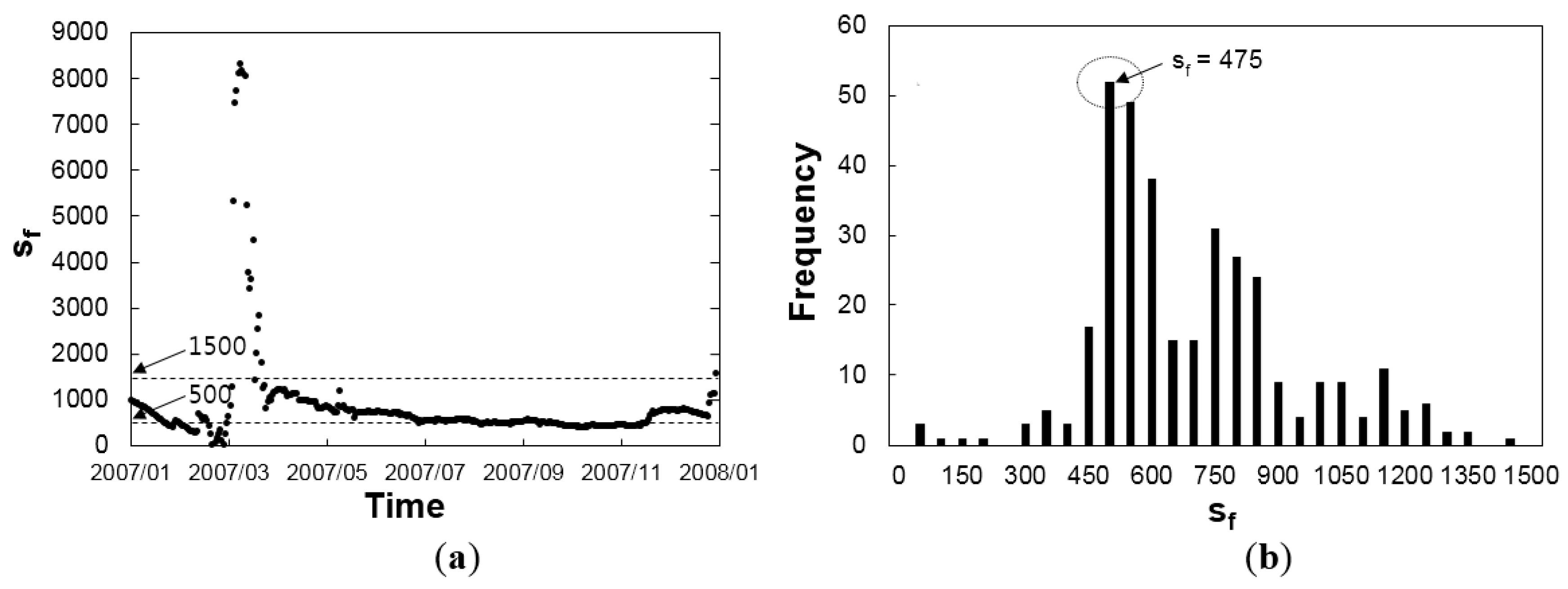
A scale factor (s_f) was introduced to adjust for differences in numerical magnitudes between GWL and moving average values. Moving average values are generally given in millimeters whereas larger units (centimeters or meters) are usually used for GWL data. The scale factor s_f then represents the ratio of daily measured GWL to the moving average value. An example of the annual distribution of s_f in 2007 obtained from region R4 is presented in Figure 13a. Most s_f values fell within the range of 500 to 1500, although some exceptionally high values of s_f were observed during the drought season from March to April. Statistical analysis of results in Figure 13a resulted in determination of the value of s_f for that year. The statistical distribution of s_f values in 2007 is shown in Figure 13b; the value of s_f with the highest frequency was 475. This s_f value of 475 was then multiplied by the t_m-day moving average to adjust for the scale difference between GWL and the moving average.

An additional calibration factor (c_f) was necessary to equalize the initial minimum values of the moving average and GWL. Note that the minimum value of the moving average could be closer to or larger than zero depending on the regional characteristics of annual precipitation. The value of c_f then corresponds to the difference between the minimum GWL and the minimum moving average for a given year, which is added to the moving average data of that year. This represents the effects of vertically shifting up the annual distribution of the moving average to ensure equality of the minimum values of GWL and the moving average. For region R4 in Figure 8a, for example, the value of c_f was 32.9. The values of t_m, s_f, and c_f were obtained for different years using the same procedure and averaged, and then used to estimate the GWL for a certain target year. The steps of the proposed method described herein are summarized in Figure 14.

Figure 13. Distributions of scale factor (s_f): (a) annual distribution and (b) statistical distribution.

Figure 13. Distributions of scale factor (s_f): (a) annual distribution and (b) statistical distribution.

Figure 14. Calculation procedure of the proposed method.

Figure 14. Calculation procedure of the proposed method.

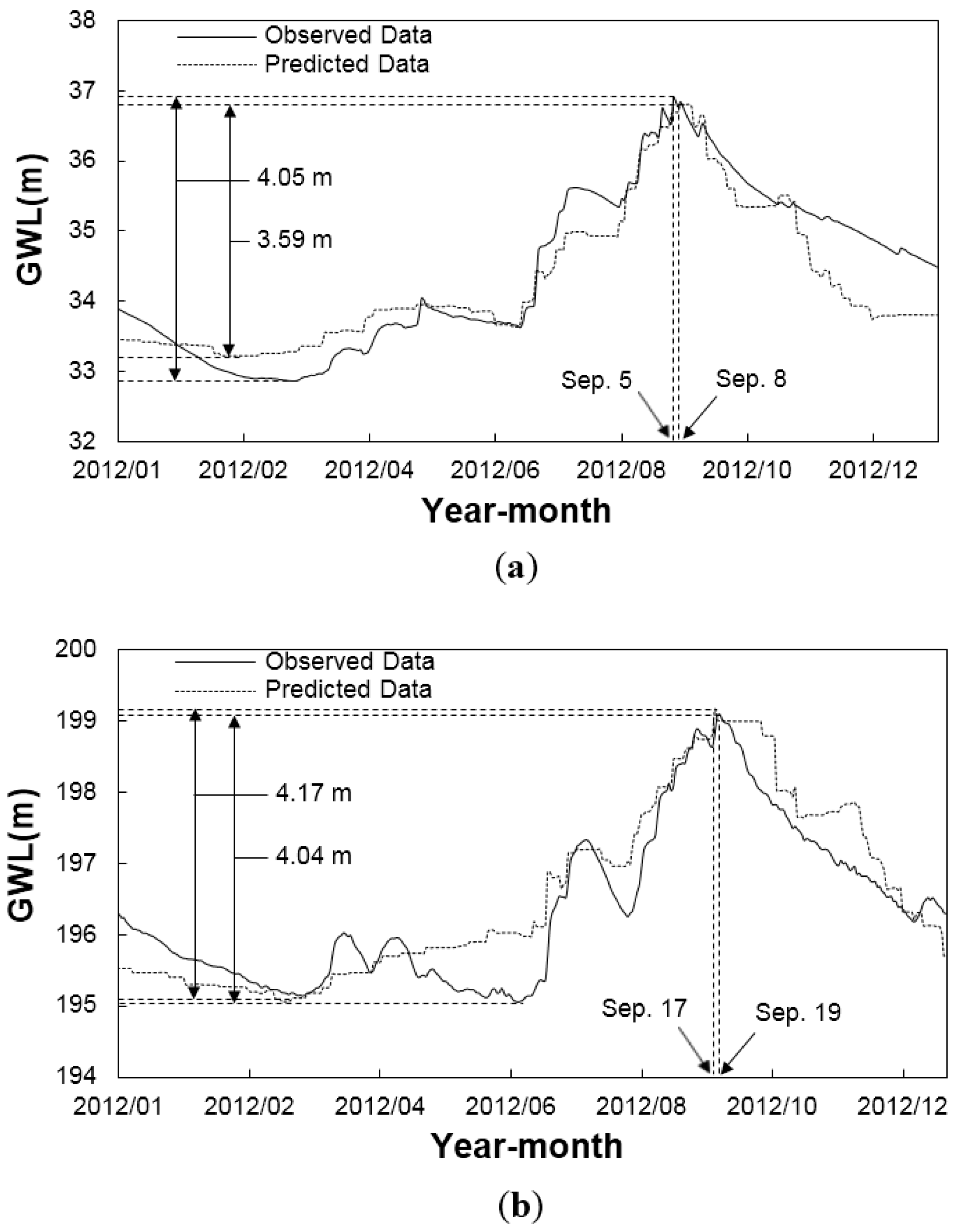
5.2.2. Measured and Predicted Groundwater Levels

To check the validity of the proposed method, the precipitation and GWL data for regions R4 and R5 from 2006 to 2011 were used to predict the GWL in 2012. Note that regions R4 and R5 belong to group C, and therefore had a low paved surface area ratio and low permeability soils. Values of t_m, s_f, and c_f obtained annually from 2006 to 2011 for regions R4 and R5 are shown in Table 5. Average values of these parameters are also included in Table 5. Using the proposed procedure described in Figure 14, the annual variations in GWL for regions R4 and R5 were predicted and compared with the measured data in Figure 15. The values of the correlation parameters t_m, s_f, and c_f used to predict the six-year average values are provided in Table 5.

Figure 15. Measured and estimated GWL variations for regions (a) R4 and (b) R5.

Figure 15. Measured and estimated GWL variations for regions (a) R4 and (b) R5.

Table 5. Correlation parameters for the proposed method.

Region	Year	2006	2007	2008	2009	2010	2011	Average
R4	tm	64	104	94	80	70	43	76
	sf	175	475	425	225	225	175	283
	cf	33.2	32.9	33.1	33.1	33.6	33.2	33.2
R5	tm	76	105	112	107	102	95	100
	sf	225	425	375	525	525	425	417
	cf	195.1	194.6	195.3	194.7	195.0	195.2	195.0

Table 5. Correlation parameters for the proposed method.

Region	Year	2006	2007	2008	2009	2010	2011	Average
R4	tm	64	104	94	80	70	43	76
	sf	175	475	425	225	225	175	283
	cf	33.2	32.9	33.1	33.1	33.6	33.2	33.2
R5	tm	76	105	112	107	102	95	100
	sf	225	425	375	525	525	425	417
	cf	195.1	194.6	195.3	194.7	195.0	195.2	195.0

Close agreements between measured and predicted GWL data for both regions were observed. The measured and predicted peak GWLs in region R4 were 36.91 and 36.80 m on 5 and 8 September, respectively, and the measured and predicted GWL fluctuations were 4.05 and 3.59 m, respectively. For region R5, the measured and predicted peak GWLs were 199.09 and 199.15 m, respectively, on 19 September, while the measured and predicted GWL fluctuations on 17 September were 4.04 and 4.09 m, respectively. The errors in GWL fluctuations between the measured and predicted data were 11.4% and 1.2% for regions R4 and R5, respectively.

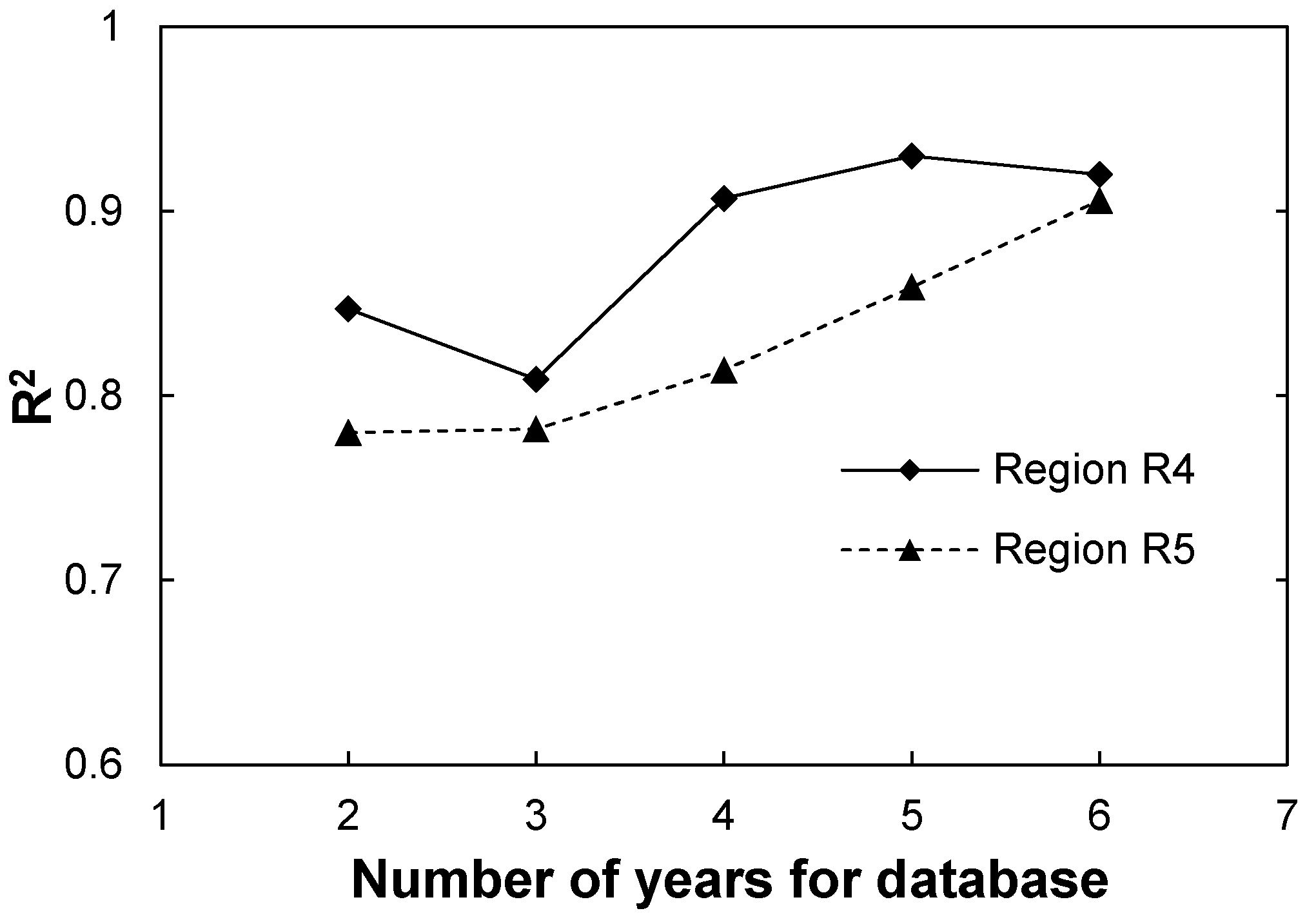
To evaluate the effect of database size on prediction accuracy, results predicted using different year databases from two to six years were obtained and compared. Figure 16 shows the values of R² for the match between measured and predicted GWL data of regions R4 and R5 in 2012. Overall, the values of R² increased as the number of years increased. For region R4, the values of R² become higher than 0.9; after 4 years, there was no significant increase in R². For region R5, the values of R² were slightly smaller than 0.8 for the two- and three-year database and then increased after four years.

Figure 16. Coefficient of correlation (R²) according to accumulation time.

Figure 16. Coefficient of correlation (R²) according to accumulation time.

6. Summary and Conclusions

Fluctuations in GWL have a negative impact on the foundations of various buildings and infrastructures due to ground subsidence and reductions in bearing capacity [5,6]. It is challenging to predict and estimate GWL and its variations, which are strongly related to meteorological characteristics [1]. In the present study, components that could potentially affect GWL were analyzed with a focus on precipitation and river stage. For this purpose, the six-year database of hydrological and groundwater monitoring results from five selected regions were obtained and adopted in the comparative analysis. Furthermore, a method for estimating GWL based on the moving average was proposed for areas with a low paved surface area ratio and soil permeability.

Correlations to the moving average were strong overall, whereas no meaningful correlation was observed with daily measured precipitation. This indicated that accumulated precipitation, which indicates the effect of preceding precipitation, was well correlated to GWL and thus a feasible parameter with which to characterize GWL. It is also observed that time lags and periods for the correlation to the moving average of the study regions differed according to soil type and local surface conditions. The correlation to river stage was highly affected by the geographic characteristics of the target region.

Key findings of this study are as follows: (1) river stage is the dominant component influencing fluctuations in GWL in urban areas with a high paved surface area ratio and near large rivers; (2) GWL of urban areas near a river is less affected by the river if the size of the river and its proximity to these areas are small; (3) for rural areas with a low paved surface area ratio and low-permeability soil, the effect of river stage on GWL is small, even if the area is located near a river. In this case, GWL is better correlated to the moving average and, accordingly, the time period that yields the best correlation should be identified; and (4) the shape and period of GWL fluctuations are affected by soil profiles and regional permeability conditions.

A simple method to estimate GWL using a moving average was proposed based on the similarity of time variation patterns of GWL and the moving average. Three correlation parameters—optimal period, scaling factor, and calibrating factor—were introduced for the proposed method and used to adjust and calibrate the GWL and moving average data. The validity of the proposed method was examined using case examples from two selected regions. It was confirmed that the proposed method can effectively predict GWL in areas with low-permeability soils and a low paved surface area ratio.

References

- Yasuhara, K.; Murakami, S.; Mimura, N.; Komine, H.; Recio, J. Influence of global warming on coastal infrastructural instability. Sustain. Sci. 2007, 2, 13–25. [Google Scholar] [CrossRef]
- Bowles, J. Foundation Analysis and Design, 2nd ed.; McGraw Hill: New York, NY, USA, 1977. [Google Scholar]
- Terzaghi, K. Theoretical Soil Mechanics; Wiley: New York, NY, USA, 1943. [Google Scholar]
- AASHTO (American Association of State Highway and Transportation Officials). Manual on Subsurface Investigations; Special Instructions to Manual on Subsurface; AASHTO: Washington, DC, USA, 1988. [Google Scholar]
- Ausilio, E.; Conte, E. Influence of groundwater on the bearing capacity of shallow foundations. Can. Geotech. J. 2005, 42, 663–672. [Google Scholar] [CrossRef]
- Shahriar, M.; Sivakugan, N.; Das, B. Settlements of shallow foundations in granular soils due to rise of water table: A critical review. Int. J. Geotech. Eng. 2012, 6, 515–524. [Google Scholar] [CrossRef]
- Shahriar, M.A.; Sivakugan, N.; Das, B.M.; Urquhart, A.; Tapiolas, M. Water Table correction Factors for settlements of shallow foundations in granular soils. Int. J. Geomech. 2014. [Google Scholar] [CrossRef]
- Almedeij, J.; Al-Ruwaih, F. Periodic behavior of groundwater level fluctuations in residential areas. J. Hydrol. 2006, 328, 677–684. [Google Scholar] [CrossRef]
- Guttman, N.B. Accepting the standardized precipitation index: A calculation algorithm. J. Am. Water Resour. Assoc. 1999, 35, 311–322. [Google Scholar] [CrossRef]
- Mohammad, A.H.; Hoque, M.M.; Ahmed, K.M. Declining groundwater level and aquifer dewatering in Dhaka metropolitan area, Bangladesh: Causes and quantification. Hydrogeol. J. 2007, 15, 1523–1534. [Google Scholar]
- Wilhite, D.A.; Glants, M.H. Understanding the drought phenomenon: The role of definitions. Water Int. 1985, 10, 110–120. [Google Scholar] [CrossRef]
- Murray, L.C., Jr. Relations between Precipitation, Groundwater Withdrawals, and Changes in Hydrologic Conditions at Selected Monitoring Sites in Volusia County, Florida, 1995–2010. U.S. Geological Survey Scientific Investigations Report 2012–5075. Available online: http://pubs.usgs.gov/sir/2012/5075/pdf/2012-5075.pdf (accessed on 24 November 2014).
- Winter, T.C. Relation of streams, lakes, and wetlands to groundwater flow systems. Hydrogeol. J. 1999, 7, 28–45. [Google Scholar] [CrossRef]
- Sanders, G. Ground Water and River Flow Analyses. Technical Report of the Platte River EIS Team 2001; U.S. Department of the Interior. Available online: https://www.platteriverprogram.org/PubsAndData/ProgramLibrary/Groundwater%20and%20River%20Flow%20Analysis.pdf (accessed on 27 November 2014).
- Kelly, P.B. Relations among River Stage, Rainfall, Ground-Water Levels, and Stage at Two Missouri River Flood-Plain Wetlands. U.S. Geological Survey Water-Resources Investigations Report 01-4123. 2001. Available online: http://mo.water.usgs.gov/Reports/01-4123-kelly/01-4123.pdf (accessed on 25 November 2014). [Google Scholar]
- KEM (Korea Environment Ministry) Website. Available online: https://egis.me.go.kr/ewebgis/webgis.jsp (accessed on 4 July 2014).
- HRBEO. Water-Environmental Management Plan of Han River in Seoul (2008~2012); Han River Basin Environmental Office: Seoul, Korea, 2007; pp. 34–37. [Google Scholar]
- GRMA (Gangwon Regional Meteorological Administration) Website. Available online: http://web.kma.go.kr/aboutkma/intro/gangwon (accessed on 14 Janrary 2014).
- HRFCO (Han River Flood Control Office) Website. Available online: http://www.hrfco.go.kr/web sumun/flood gate.do (accessed on 12 November 2013).
- NGIC (National Groundwater Information & Service Center) Website. Available online: https://www.gims-.go.kr/monitor3/ (accessed on 10 June 2014).
- Ha, K.; Ko, K.; Koh, D.; Yum, B.; Lee, G. Time series analysis of the responses of the groundwater levels at multi-depth wells according to the river stage fluctuations. Econ. Environ. Geol. 2006, 39, 269–284. [Google Scholar]
- Larocque, M.; Mangin, A.; Razack, M.; Banton, O. Contribution of correlation and spectral analysis to the regional study of a large karst aquifer. J. Hydrol. 1998, 205, 217–231. [Google Scholar] [CrossRef]
- Lee, J.; Lee, K. Use of hydrologic time series data for identification of recharge mechanism in a fractured bedrock aquifer system. J. Hydrol. 2000, 229, 190–201. [Google Scholar] [CrossRef]
- Park, J.; Choi, Y.; Kim, D.; Park, C.; Yang, J. Development of groundwater dam operation index using daily precipitation data. In Proceedings of the Workshop of Korea Water Resources Association, Jeju, Korea, October 2005; p. 60.
- Booh, S.; Shin, S.; Choi, Y.; Park, J.; Jeong, G.; Park, C. Operation strategy of groundwater dam using estimation technique of groundwater level. KCID J. 2006, 13, 48–57. [Google Scholar]
- Box, G.; Jenkins, G. Time Series Analysis: Forecasting and Control; Holden Day: San Francisco, CA, USA, 1976; p. 575. [Google Scholar]
- Laux, P.; Vogl, S.; Qiu, W.; Knoche, H.; Kunstmann, H. Copula-based statistical refinement of precipitation in RCM simulations over complex terrain. Hydrol. Earth Syst. Sci. 2011, 15, 2401–2419. [Google Scholar] [CrossRef] [Green Version]
© 2015 by the authors; licensee MDPI, Basel, Switzerland. This article is an open access article distributed under the terms and conditions of the Creative Commons by Attribution (CC-BY) license (http://creativecommons.org/licenses/by/4.0/).