Bayesian Analysis of Demand Elasticity in the Italian Electricity Market

Abstract

The liberalization of the Italian electricity market is a decade old. Within these last ten years, the supply side has been extensively analyzed, but not the demand side. The aim of this paper is to provide a new method for estimation of the demand elasticity, based on Bayesian methods applied to the Italian electricity market. We used individual demand bids data in the day-ahead market in the Italian Power Exchange (IPEX), for 2011, in order to construct an aggregate demand function at the hourly level. We took into account the existence of both elastic and inelastic bidders on the demand side. The empirical results show that elasticity varies significantly during the day and across periods of the year. In addition, the elasticity hourly distribution is clearly skewed and more so in the daily hours. The Bayesian method is a useful tool for policy-making, insofar as the regulator can start with a priori historical information on market behavior and estimate actual market outcomes in response to new policy actions.

1. Introduction

The Italian electricity sector was transformed by a deregulation process into a competitive market, overcoming the previous system which was based upon a vertically integrated monopoly, owned by the State. This process led to the institution of the Power Exchange (IPEX) in 2004, aimed at promoting competition in generation activities. The transition was not simple because the definition of a proper market structure preserving competition is not an immediate undertaking.

The goal of enhancing competition involves limiting the exercise of market power in the supply chain.

Market power can be defined as the ability of a supplier to profitably raise prices below the competitive level by reducing output below the competitive level. Under the assumptions of perfect competition, companies are in fact price takers: any minimal increase in the price would lead to negative profits, given that potential buyers could make the other competitors (offering lower price) cover their demand. When the market is not competitive, companies are price makers since they can raise the price without loss, causing a decrease in the quantity demanded and an associated sub-optimal state compared to the conditions of perfect competition. The exercise of market power has important implication in terms of efficiency [1].

In the short-run, it affects productive efficiency since the reduction of the output to raise prices leads smaller players (with higher generation costs) to expand generation from more expensive plants in response to the higher prices.

In the medium or long-run market power causes allocative inefficiencies. In particular, the marginal value of the next unit of consumption will be in excess of the marginal cost of some units of withheld supply. Moreover, market power can increase the level of congestion on a network, thereby affecting efficiency and reliability of the system. Finally, market power can affect long-term decisions: an increase in power prices should ideally be interpreted as a signal for investors that new capacity is needed, but this may not be the case if market power is being exercised.

Given all these implications, the design of the deregulated electricity markets offers a challenging opportunity to analyze the main design frameworks and their effects on the functioning of the electricity pool market and the consumer price reaction [2,3].

From a theoretical modeling standpoint, the elasticity of the demand curve is the crucial factor that determines whether and how a company can increase the sale price above the marginal cost without incurring losses.

Looking in fact at one of the most widely used index measuring market power, the Lerner index, the direct link between market power and demand elasticity is immediately highlighted. According to this index, the markup of a company (the difference between the charged price and marginal costs) is inversely related to the elasticity of the market demand.

Given the purpose of the Italian Regulator of preserving competition and efficiency in the electricity market, investigation of demand elasticity becomes essential to identify the design factors to be used for the definition of the market structure; the consumer reactivity to changes in price can express market efficiency as expressed in reference [4]. Then, in strategic economic sectors, this measure can be seen as a tool leading the National Regulators in the market structure definition processes. While the supply side of the electricity markets has been extensively analyzed, we believe that the behavior of the demand side has been of much less interest. Most studies have tried to study market power in the electricity sector applying oligopolistic models: reference [5] implemented a Cournot market with a competitive fringe for California Power Exchange, while reference [6] compared two oligopolistic models (the Supply Function and the Cournot model for the German Power Exchange data) identifying the Cournot model as the best fitting model. For a survey of the most relevant publications regarding electricity market modelling, see reference [7].

The analysis of elasticity and the competitive structure of the electricity market using demand data has not been so popular. We mention the work of Patrick and Wolak who tried to present estimates of the customer-level demand for electricity by industrial and commercial customers purchasing electricity using the half-hourly energy prices from the England and Wales electricity market [8].

The traditional stylized fact is that buyers in the electricity markets are primarily distributors, who are passive intermediaries of the final consumption demand. It seems appropriate also taking into account the spread of distributed generation, as a result, in particular, of photovoltaic and cogeneration plants connected with the electrical grid; the causes and consequences of distributed generation connected with the electrical system in Italy are shown in reference [9]. In reality, a significant proportion of buyers in the Italian market is made up of large heavy-energy consuming industrial users, such as steel, cement, chemicals, pulp and paper, who are certainly elastic to hourly price patterns, at least to some extent. This behavior is precisely what we want to analyze, and the aim of this paper is to provide a new estimate of the elasticity of the demand of the Italian electricity market, using Bayesian techniques.

We believe that in the electricity market, there are specific technical features, which influence the competitive outcome of supply and demand interplay. These are mainly constituted by the technical constraints of the transmission network.

In the grid operation there is the need for instantaneously and continuously balancing the flows injected into and withdrawn from the grid. For a deep analysis of the main characteristics of the real-time operation of the electricity system and the alternative design of balancing arrangements see reference [10] and for the comprehensive classification of different market systems and for the cost-benefit analysis of demand response (DR) programs among which the Regulator can choose see references [11,12]. Frequency and voltage on the grid must be kept within a very narrow range, so as to protect the security of installations. The management of the transmission network must ensure that the power flows on each line do not exceed the maximum admissible transmission capacity (transmission or transit limits) of the same line.

In addition, power demand is remarkably variable both in the short term (hourly) and in the medium term (weekly and seasonal). The electric system lacks storage for adjustments of supply, because it is impossible to store electricity in a significant and economically feasible way.

Power generation units have minimum and maximum generating capacity limits, as well as a minimum switching-on time and a minimum generating capacity adjustment time. Electricity flows through all the available lines, like in a system of communicating vessels, under complex physical laws that depend on the equilibrium between injections and withdrawals; hence, the path of electricity is not traceable and, if a local imbalance is not promptly redressed, it will propagate to the overall grid inducing frequency and voltage perturbations, which can result in black-outs.

The Electricity Market was reformed in Italy empowering new specialized institutions, owned by the State, with the aim of promoting competition in the activities of electricity generation and wholesale price formation. At the same time, market design promoted the efficiency maximization in the naturally monopolistic activity of dispatching. This reform was established in 1999 in the wider context of the electricity sector liberalization process.

The transmission system operator function was assigned to “Terna S.p.A.”, which is the company in charge of the Italian national grid. The market operator function was assigned to the “Gestore dei Mercati Energetici S.p.A.” (GME), which is the company in charge of organizing and managing the electricity market, the natural gas market and the environmental markets in Italy under the principles of neutrality, transparency, objectivity, and competition among or between producers. Its mission is to promote the development of a competitive national power system.

The reform also created the Single Buyer, “Acquirente Unico S.p.A.”, with the task of guaranteeing the availability of electricity to cover the demand of Captive Customers. It operates by purchasing the required electrical capacity, reselling it to distributors on non-discriminatory terms, and making possible the application of a single national tariff to customers.

There are several organized markets managed by GME, which are the spot electricity market (MPE), the forward electricity market with delivery-taking/-making obligation (MTE) and the platform for physical delivery of financial contracts concluded on IDEX (CDE).

Unlike other European energy markets, GME’s market is not a merely financial market, where prices and volumes only are determined, but a real market, where physical injection and withdrawal schedules are defined.

GME’s market reflects the segmentation of transmission grids (“zones”) where, for purposes of power system security, there are physical limits to transmission of electricity to/from the corresponding neighboring zones. These transmission limits are determined through a computational model that is based on the balance between electricity generation and consumption.

The zones of the “relevant grid” may correspond to physical geographical areas, to virtual areas (i.e., not directly corresponding to physical areas) or to points of limited production (virtual zones whose generation is subject to constraints aimed at maintaining the security of the power system); to identify and remove any congestion which may be caused by injection or withdrawal schedules—whether defined in the market or implementing bilateral contracts. The configuration of these zones depends on how Terna manages the flows along the peninsula. These zones may be summarized as follows:

-

six geographical zones (central-northern Italy, northern Italy, central-southern Italy, southern Italy, Sicily, and Sardinia);

-

eight neighboring countries’ virtual zones (France, Switzerland, Austria, Slovenia, BSP, Corsica, Corsica AC, and Greece);

-

four national virtual zones representing constrained zones, i.e., zones consisting only of generating units, whose interconnection capacity with the grid is lower than their installed capacity.

The spot electricity market is divided in three specific submarkets: the Day-Ahead Market (MGP), where producers, wholesalers and eligible final customers may sell/buy electricity for the next day; the Intra-Day Market (MI), which replaced the existing Adjustment Market, organized into four sessions, where producers, wholesalers and eligible final customers may change the injection/withdrawal schedules determined in the MGP; the Ancillary Services Market (MSD), where Terna S.p.A. procures the ancillary services needed to manage, operate, monitor, and control the power system.

The analysis of this paper concerns data from the most prevalent submarket of the MPE: the Day-Ahead Market (MGP). It is an electronic venue for wholesale trading, where hourly blocks of electricity are negotiated, hourly prices and volumes are defined through the intersection between demand and supply curve. In this market, electricity is traded by scheduling generating and consuming units; the MGP session opens at 8 a.m. on the ninth day before the delivery-day and closes at 9.15 a.m. on the day before the delivery is executed.

During the session, market participants may submit bids/offers where they specify the volume and the maximum/minimum price at which they are willing to purchase/sell. Supply offers and demand bids must correspond to the real willingness to inject or withdraw the related volumes of electricity.

The MGP is organized according to an implicit double auction where bids/offers are accepted under the economic merit-order criterion and subjected to transmission limits between zones.

The market algorithm will accept bids/offers in such a way as to maximize the value of transactions, given the maximum transmission limits between zones. Supply offers are ranked in increasing price order on an aggregate supply curve while all valid and adequate demand bids that have been received are ranked in decreasing price order on an aggregate demand curve. The intersection of the two curves gives: the overall traded volume, the clearing price, the accepted bids/offers, and the injection and withdrawal schedules obtained as the sum of the accepted bids/offers pertaining to the same hour and to the same offer point.

If any transmission limit is not violated, the clearing price is a single clearing price P* for all the zones. Accepted bids/offers are those having a selling price not higher than P* and a purchasing price not lower than P*.

If at least one limit is violated, the algorithm performs market splitting, i.e., the market is divided into two market zones, namely, one exporting zone, including all the zones upstream of the constraint, and one importing zone, including all the zones downstream of the constraint. In each zone, the algorithm repeats the above-mentioned intersection process until no transmission constraints are violated. The result is a zonal price differentiation.

With regard to the price of electricity allocated for consumption in Italy, GME applies a national single purchasing price (PUN), which is equal to the average of zonal selling prices weighted for zonal consumption, whereas accepted offers to sell are evaluated at the zonal price Pz. An extensive literature explores the auctions in the energy markets and investigates their connection with market power, collusion, efficiency, and consumer welfare, all of them with notable policy implications. An efficient electricity double-sided auction mechanism should control market power. Participants may play a pivotal role, which is a critical factor in the determination of the market clearing price and in exercise of the market power (see [13]).

2. Experimental Section

We used GME’s daily data gathered in the monthly dataset starting from January 2011 to December 2011. Each monthly dataset accounts for 1.5 million raw observations.

2.1. Materials and Data

The main variables characterizing each raw observation are:

• Purpose: Purpose of BID or OFF, where BID pertains to the participant’s purchases and OFF to the participant’s sales.
• Interval: The relevant period to which the bid or the offer refers.
• Bid Offer Date: The flow date of the bid or the offer.
• Operator: The registered name of participant.
• Zone: The zone to which the unit belongs.
• Bilateral: This is a categorical variable that indicates whether the bid or the offer comes from the wholesale market or a bilateral contract.
• Quantity: The volume submitted by participants
• Energy Price: The price submitted by participants.

We retained only the observations referring to the demand side (BID). In each monthly dataset, there are about 400–450 thousand observations on bids, accounting for the 20%–25% of the total amount of the raw dataset. We balanced the datasets in order to obtain the same number of hourly observations within each month. We constructed the aggregated demand curves for each hour of the day. Bids representing inelastic behavior were lumped into one aggregated observation, defining the vertical intercept of the aggregate demand curve. At the end of procedure the sample size of the monthly balanced dataset ranged from 15,558 observations (recorded in February 2011) to 23,148 observations recorded in November 2011.

The preliminary investigation of the datasets is to provide an exhaustive analysis of the Day-Ahead Market highlighting its main features.

Firstly, datasets contain observations where the price is not specified, expressing the maximum willingness to pay (that is lower responsiveness to a change in the energy price). Since buyers are willing to pay any price resulting from the market clearing mechanism, being not aware of the market price signals, they have a perfectly inelastic behavior. GME assigns to these bids a fictitious price equal to the supply price cap that is equal to 3000/MWh. Table 1 show that these bids are about 80% of the total bids with respect to the frequency and the hourly average share.

Table 1. Hourly average absolute frequency and hourly average quantity bid. Elastic and inelastic bid.

2011	Average Absolute Frequency		Average Quantity Bid
	Inelastic Bid	Elastic Bid	Inelastic Bid	Elastic Bid
Peak	419.53	9.22	94.37	13.86
Off-peak	426.63	10.25	73.21	13.43

Table 1. Hourly average absolute frequency and hourly average quantity bid. Elastic and inelastic bid.

2011	Average Absolute Frequency		Average Quantity Bid
	Inelastic Bid	Elastic Bid	Inelastic Bid	Elastic Bid
Peak	419.53	9.22	94.37	13.86
Off-peak	426.63	10.25	73.21	13.43

Secondly, we have to mention the portion of bids referring to the Italian Single Buyer, whose hourly average demand share proxies the portion of electricity demand satisfying captive and domestic buyers. Single Buyer covers a big portion of demand. Moreover, variation of quantity shares between peak and off peak hours may suggest that captive buyers change their consumption profile during the day. Table 2 shows that the hourly average share covered by a Single Buyer is about 15% of the hourly equilibrium demand. Moreover, the Italian Power Exchange is a voluntary market: purchase and sale contracts may also be concluded off the exchange platform, i.e., bilaterally or over the counter (OTC). Table 2 demonstrates that the share covered by bilateral contracts on average accounts for half of the equilibrium quantity.

Transmission constraints influence the equilibrium prices on both the supply and the demand side. On the supply side, congestion is resolved with market splitting yielding a zonal differentiation of the prices. On the demand side, congestion affects the single national price, since the price paid by buyers is the weighted average of zonal prices formed on the supply side.

Table 2. Single Buyer and bilateral contracts, hourly average share and frequency.

2011	Single Buyer		Bilateral Contract
	Average Frequency	Average Share	Average Frequency	Average Share
Peak	0.53%	17.02%	52.70%	46.60%
Off-Peak	0.40%	12.58%	52.07%	50.27%

Table 2. Single Buyer and bilateral contracts, hourly average share and frequency.

2011	Single Buyer		Bilateral Contract
	Average Frequency	Average Share	Average Frequency	Average Share
Peak	0.53%	17.02%	52.70%	46.60%
Off-Peak	0.40%	12.58%	52.07%	50.27%

Table 3 shows the frequency of the different market splitting occurring for 2011. In 2011, the one zone market occurred 15% of the times. Market splitting in two zones was the most frequent occurrence, 47% of the hours, while splitting in four zones was marginal and occurred on average just 3% of the times. Market segmentation in five zones has not been taken in consideration since it never occurred in 2011.

Table 3. Frequency congestion.

Congestion	Average Frequency
2011
Number of Zone	1	2	3	4
	15%	47%	35%	3%

Table 3. Frequency congestion.

Congestion	Average Frequency
2011
Number of Zone	1	2	3	4
	15%	47%	35%	3%

Finally Table 4 and Table 5 show the PUN pattern during peak and off-peak hours, respectively, according to the market splitting, demonstrating the correlation between congestion and the recorded level of equilibrium price. In 2011, PUN reached higher values when three-zone segmentation occurred (both peak and off-peak hours).

When congestion occurs, the demand equilibrium price tends to increase confirming that the absence of congestions improves market efficiency. Furthermore, it highlights how investments in transmission capacity are one of the major concerns, given the crucial role played by electricity in national economic activities.

Table 4. National single purchasing price (PUN) by market segmentation, peak hour.

Zone	Peak Average PUN
	Mean	Stand. Dev.	Min	Max
1	76.67	20.08	47.00	160.00
2	78.26	14.01	31.00	164.80
3	82.59	14.62	50.48	161.99
4	78.11	12.19	59.53	119.64

Table 4. National single purchasing price (PUN) by market segmentation, peak hour.

Zone	Peak Average PUN
	Mean	Stand. Dev.	Min	Max
1	76.67	20.08	47.00	160.00
2	78.26	14.01	31.00	164.80
3	82.59	14.62	50.48	161.99
4	78.11	12.19	59.53	119.64

Table 5. PUN by market segmentation frequency, off-peak hour.

Zone	Off-Peak Average PUN
	Mean	Stand. Dev.	Min	Max
1	56.77	12.22	10.00	115.00
2	71.46	14.82	17.86	137.84
3	64.27	14.92	10.00	127.71
4	57.28	11.17	28.08	94.81

Table 5. PUN by market segmentation frequency, off-peak hour.

Zone	Off-Peak Average PUN
	Mean	Stand. Dev.	Min	Max
1	56.77	12.22	10.00	115.00
2	71.46	14.82	17.86	137.84
3	64.27	14.92	10.00	127.71
4	57.28	11.17	28.08	94.81

2.2. Method and Theoretical Framework

In the Italian wholesale electricity market only eligible buyers can operate and they are large buyers (energy intensive industries, railways, telecom companies), industrial buyers, and traders who can intermediate both large, small industrial and residential consumers (households).

We adopted an econometric approach coherent with the neoclassical framework of rational optimizing behavior. In the energy demand analysis, a large variety of methods can be used, ranging from end-use approach to input-output models. For a review and comparative analysis of alternative approach in the electricity market modelling, see reference [14].

Eligible buyers use electricity as an input in the production function to produce goods and services, within a cost minimization process. We assume that buyers rationally behave minimizing their hourly expenditure function:

$$C=c\left(p, Q\right)$$

(1)

where $p$ is the vector of prices of all the goods needed to run their economic activities and $Q$ is the objective variable to be maximized as the level of output they want to reach.

Under the given assumptions, solving the problem using the Lagrangian method yields the system of equation called Hicksian demand functions, where the quantities demanded for each good are expressed in terms of prices and the objective variable:

$$\frac{\partial C\left(Q,p\right)}{\partial p_i}=h_i\left(Q,p\right)=q_i$$

(2)

These functions are called compensated demand equations because they consider the objective variable Q as a constant parameter. As suggested by reference [15], for generating empirically useable models, dual representations are typically most convenient. The empirical work required in fact to cast the economic optimization problem in a model, where quantities are a function of prices and total expenditure. The duality approach allows shifting from the production possibility sets (and the system of preferences) to the market demand function.

Introducing the inverse function of the objective variable $V\left(m,p\right)=\text{Q}$ where $m$ is the budget constraint and substituting in V the budget constraint with the expenditure function, we have:

$$\text{Q}=V\left(m,p\right)=V\left(C\left(p,Q\right),p\right)$$

(3)

We assume that the cost function is continuous, increasing in Q, non-decreasing, linearly homogeneous and concave in prices. If we differentiate V with respect to price:

$$\frac{\raisebox{1ex}{$\partial V$}\!\left/ \!\raisebox{-1ex}{$\partial p_i$}\right.}{\raisebox{1ex}{$\partial V$}\!\left/ \!\raisebox{-1ex}{$\partial C$}\right.}=h_i\left(Q,p\right)=g_i\left(m,p\right)$$

(4)

We obtain the Roy identity, i.e., Marshallian demands $g_i\left(m,p\right)$ expressing quantity of an input or good as a function of its own price, the budget constraint and the price of all the other goods.

The multidimensional model needs to be reduced into a two dimensional problem. For this reason, all the other goods and inputs are bundled in a numeraire good that is evaluated at a price proxied by the monthly consumer price index (adjusted, excluding from its computation the energy consumption).

We use a log-linear demand function where the dependent variable is the logarithm of aggregated demand and the explanatory variables are the corresponding logarithm of prices, adjusted by the monthly consumer index price (representing the price of the numeraire) and dummy variables (relative to the day the zone etc.) which approximate the total expenditure.

$$log{y}_i={\alpha }_i+{\beta }_i\text{log}\left(\frac{p_i}{\overline{p}}\right)+{{\displaystyle \sum }}^{\text{}}{\gamma }_{ki}{d}_{ki}$$

(5)

In spite of the proliferation of flexible functional forms for consumer demand systems, the double-log demand model continues to be popular, especially in applied work calling for single-equation models [16]. However, alternative models used for consumer demand analysis, as Rotterdam and AIDS models can be found in references [17] and [18].

There are three relevant issues to be analyzed more in depth in order to correctly interpret such a theoretical demand model in the framework of the Italian electricity market.

Firstly, agents who submit demand bids are not necessarily final users of electricity, they can be intermediary agents who submit demand bids on behalf of final customers, buying electricity from the market and reselling it to distributors. The role of traders (in particular Single Buyer) should be processed into the model as a principal-agent relationship where the principals are the final users. Secondly, opportunistic behavior, as arbitraging between Day-Ahead Market and Infra-Day Market, may be expected. However, institutional market factors suggest the impossibility for agents to have strategic behavior. Arbitraging is not convenient because the National Market Regulator imposes penalty charges if the real loads deviate from the withdrawal profiles defined in the Day-Ahead Market. For this reason traders have to submit bids reflecting their real willingness to pay. Since the agent’s incentives are consistent with the principal’s interest, the resulting equilibrium is Pareto-Optimal. Thirdly, there are heterogeneous final consumers, some of who pay a contract price and are not necessarily aware of the hourly price signal in the wholesale market.

There are two types of bidding behavior in the MGP. We label type 1 behavior as those bids specifying a definite price. This behavior is considered referring to an elastic behavior with non-zero elasticity demand: y₁ = f(p₁) with elasticity ε₁ < 0. This elastic buyer has a reservation price, which is lower than the maximum price attributed to the inelastic buyer.

We label type 2 behavior as those bids referring to bilateral contracts, which do not specify any price. These bids are recorded by the GME as bids with a fictitious price equal to the supply price cap, set at 3000 euro/MWh. These bids represent the maximum willingness to pay and characterize perfectly inelastic behavior. Empirically, these bids with no price are gathered into a demand category denoted by an inelastic demand function: y₂ = f(p₂) with elasticity ε₂ = 0.

If the equilibrium price is greater than the reservation price of the elastic buyer then the market demand is expressed only by elasticity of the type 2: ε₂ is equal to zero and this means that the market outcome is not influenced by demand elasticity.

On the contrary, if the equilibrium price is lower than the reservation price of the elastic buyer, then the market demand is given by the aggregation of both types of buyers and its elasticity will be expressed by the negative elasticity of type 1: ${\text{ε}}_1$.

2.3. Statistical Model

We assume that the day is divided into two groups of hours (peak and off-peak hours), one ranging from 9 a.m. to 8 p.m. (the time period in which the majority of consumption and economic activities take place), the second instead goes from 9 p.m. to 8 a.m.

Hourly average demand gives evidence of the assumption of a differentiated group of hours; the off-peak electricity demand profiles substantially differ from those recorded during peak hours; since some economic activities cannot be run, electricity demand is lower. The total quantity submitted in off-peak hours is on average 25% lower than the total quantity recorded in a peak hour.

Differences can be noticed even in Market Equilibrium Prices (PUN): during peak hours, as demand is higher, equilibrium price is higher. Tables below show summary statistics of hourly average PUN aggregated within peak/off-peak group of hours.

The behavior analysis of industrial buyers and traders is undertaken using a multivariate linear regression model. Since in the wholesale (electricity) market hourly blocks of electricity are traded, we computed the estimates of the hourly demand elasticities.

We regressed the hourly logarithm of electricity demand on the adjusted logarithm of price and other explanatory variables as proxy expenditure availability. Within explanatory variables approximating total expenditure, we mentioned the daily dummies, which allowed us to recover hourly beta’s estimates.

Multiple equations regression model (SUR model) is required since we want to analyze if the economic agents, given rational expectation of changes in price are able to modify their electricity profiles within a given time slot. For an overview of the underlying SUR model see reference [19].

We divided the day into two groups of hours (peak and off-peak) and we blocked together the hourly aggregated demand vectors assuming that the hourly optimal demand chosen by buyers is correlated with each other within the same group of hours.

$$y_{mi}={\beta }_{m1}{x}_{mi1}+{\beta }_{m2}{x}_{mi2}+\dots +{\beta }_{mK}{x}_{miK}+{\epsilon }_{mi}$$

(6)

where $i=1,\dots ,N$ are the observations and $m=1,\dots ,12$ are the equations. The variable $y_{mi}$ is the i-th observation of the dependent variable (the log-demand) in equation m, $x_{mik}$ (with k = 1, ..., K) is the i-th observation of the k-th explanatory variable of the m-th equation and ${\beta }_{mk}$ is the k-th regression coefficient of the m-th equation.

The analysis is cast within a Bayesian framework to be later compared with the estimation results obtained by the frequentist approach.

We denote: $y_m=\left[\begin{array}{ccc}{y}_{m1}& \dots & y_{mN}\end{array}\right]\text{’}$; ${\epsilon }_m=\left[\begin{array}{ccc}{\epsilon }_{m1}& \dots & {\epsilon }_{mN}\end{array}\right]\text{’}$; $X_m=\left[\begin{array}{ccc}x{\text{′}}_{m1}& \dots & x{\text{′}}_{mN}\end{array}\right]\text{’}$;

${\beta }_m=\left[\begin{array}{ccc}{\beta }_{m1}& \dots & {\beta }_{mK}\end{array}\right]\text{’}$ so that we can write the model in a compact form:

$$Y=\left[\begin{array}{c}{y}_1\\ y_2\\ \begin{array}{c}⋮\\ y_M\end{array}\end{array}\right], \epsilon =\left[\begin{array}{c}{\epsilon }_1\\ {\epsilon }_2\\ \begin{array}{c}⋮\\ {\epsilon }_M\end{array}\end{array}\right], X=\left[\begin{array}{c}{X}_1\dots \dots 0\\ 0X_2\dots 0\\ \begin{array}{c}⋮\\ 0\dots \mathrm{..}{X}_M\end{array}\end{array}\right],\beta =\left[\begin{array}{c}{\beta }_1\\ {\beta }_2\\ \begin{array}{c}⋮\\ {\beta }_M\end{array}\end{array}\right]$$

$$Y=X\beta +\epsilon$$

(7)

where $\epsilon ~N\left(0,\Omega \right)$ and $\Omega =\text{Σ}\otimes I_N$, denoting, as usual, the overall model covariance matrix as the Kronecker product of the contemporaneous covariance matrix and time identity matrix.

In the Bayesian framework, we want to assess which random mechanism generates the data, given the sample. The parameter indexing the distribution generating data is in fact a random variable (see references [20] and [21]). This randomness depends on the fact we have uncertain knowledge about its value and this uncertainty is expressed giving a probability distribution to the parameter. This distribution is called prior and it is subjective since it originates from pre-experimental information. After observing the experimental results, which are the samples drawn from the distribution indexed by the parameter we want to estimate, we compute the likelihood function (the conditional probability of the sample given the parameter).

Then, these two main features of Bayesian inference, prior and likelihood, are combined together using Bayes Theorem and lead to inverse probability distribution called posterior distribution. It represents the distribution of the parameter after observing the experimental data. The joint posterior distribution describes our assessment of where the true values of parameters are likely to lie in the parameter space after observing the sample. The Bayes rule describes how prior knowledge is updated by the sampling.

Following the Bayesian framework proposed by Koop in reference [22], for $\beta$ and $\Sigma$ we chose semi-conjugate priors: $p\left(\beta ,\Sigma \right)=p\left(\beta \right)p\left(\Sigma \right)$. We assume that $\beta$ follows a Multivariate Normal distribution: $p\left(\beta \right)~N\left({\beta }_0,V_0\right)$, while for the variance of the model we assume an inverse Wishart Distribution: $p\left(\Sigma \right)~I{W}_{{\nu }_0}\left({{\Lambda }_0}^{-1}\right)$. Prior hyper-parameter elicitation comes from the previous empirical study, then, for the beta parameters, the Normal Prior distribution is centered on the frequentist hourly estimates referring to the previous year (2010) computed by reference [23].

Applying Bayes rule we obtained the posterior distribution for beta and sigma:

$$p\left(\beta ,\Sigma |y\right)\propto exp\left\{{\displaystyle \sum }_i-\frac{1}{2}{A}_i\right\}\times |V_0{|}^{-1}exp\left\{-\frac{1}{2}B\right\}\times {\left|\Sigma \right|}^{-\frac{1}{2}\left({\nu }_0+M+1\right)}exp\left\{-\frac{1}{2}tr\left({\Lambda }_0{\Sigma }^{-1}\right)\right\}$$

(8)

where:

$A_i=\left(y_i-X_i\beta \right)\prime {\Sigma }^{-1}\left(y_i-X_i\beta \right)$, with i = 1, …, N;

$\text{B}=\left(\beta -{\beta }_0\right)\prime {V_0}^{-1}\left(\beta -{\beta }_0\right)$

Since posterior distribution is not identifiable as a well-known distributional form, we use the two full conditional $p\left(\beta |\Sigma ,y\right)$ and $p\left(\Sigma |\beta ,y\right)$. distributions to run Gibbs Sampling and simulate the posterior distribution from them:

$$p\left(\beta |\Sigma ,y\right)~N\left({\beta }_n,V_n\right)$$

(9)

$$p\left(\Sigma |\beta ,y\right)~I{W}_{{\nu }_n}\left({{\Lambda }_n}^{-1}\right)$$

(10)

where

$$V_n={({V_0}^{-1}+{\displaystyle \sum }_i^n{X}_i{\Sigma }^{-1}{X}_i)}^{-1}$$

$${\beta }_n=V_n\left({V_0}^{-1}{\beta }_0+{\displaystyle \sum }_i^n{X}_i{\Sigma }^{-1}{y}_i\right)$$

$${\nu }_n={\nu }_0+n$$

$${\Lambda }_n={\Lambda }_0+{\displaystyle \sum }_{i=1}^n\left(y_i-X_i\beta \right)\left(y_i-X_i\beta \right)\prime$$

Gibbs Sampler produces samples from the joint posterior distribution by constructing a Markov Chain whose transition kernel uses the two full conditional distributions. The chain converges to the posterior distribution, which is its unique stationary limiting distribution, for the transition matrix which satisfies the detailed balanced condition. See references [24,25].

The first 1000 observations were as a burn-in period to avoid the chain to be dependent on the starting value. The remaining sequence of 10,000 draws $\left\{{\beta }^{\left(i\right)}\prime ,{\Sigma }^{\left(i\right)}\prime \right\},$ simulates a sample from $p\left(\beta , \Sigma |y\right)$.

3. Results and Discussion

All computational procedures were performed using R 3.0 and MATLAB 7.12.0 software. Useful for the implementation of codes were the references [26,27].

Posterior means of betas were computed using Lesage codes in MATLAB [28].

Firstly, it can be noticed that average elasticities vary within the hours of the day, month, and the year. Looking at Table 6, estimates in 2011 range from a minimum value of −0.0019 (registered on 10 p.m. of August) to −0.1952 recorded in March at 4 a.m.

In the following, we refer to values of the elasticities in absolute terms, given that demand elasticities are usually negative. Therefore, we refer to “higher elasticity”, when the absolute value is higher even if the algebraic number is more negative and therefore “lower”.

Elasticities are generally higher during the off-peak hours as shown by Table 7 and Table 8 with some exceptions in the month of April, July, August, and October. The skewness of the estimates is negative in each hour of the day showing that the tails on the left side of the probability density functions are longer.

Table 6. Hourly average elasticity by month.

	Hour	January	February	March	April	May	June	July	August	September	October	November	December
Peak	9	−0.024	−0.043	−0.115	−0.096	−0.073	−0.033	−0.057	−0.061	−0.036	−0.074	−0.028	−0.043
	10	−0.056	−0.109	−0.071	−0.091	−0.142	−0.046	−0.060	−0.056	−0.033	−0.079	−0.030	−0.049
	11	−0.048	−0.110	−0.047	−0.086	−0.062	−0.037	−0.061	−0.063	−0.019	−0.088	−0.034	−0.043
	12	−0.059	−0.111	−0.115	−0.066	−0.057	−0.037	−0.055	−0.079	−0.021	−0.047	−0.041	−0.046
	13	−0.051	−0.097	−0.076	−0.068	−0.151	−0.035	−0.057	−0.065	−0.023	−0.060	−0.110	−0.037
	14	−0.062	−0.113	−0.121	−0.072	−0.148	−0.029	−0.068	−0.084	−0.026	−0.072	−0.043	−0.043
	15	−0.049	−0.079	−0.114	−0.071	−0.162	−0.036	−0.048	−0.071	−0.023	−0.046	−0.031	−0.041
	16	−0.044	−0.023	−0.108	−0.074	−0.077	−0.019	−0.070	−0.063	−0.024	−0.061	−0.039	−0.044
	17	−0.035	−0.079	−0.074	−0.077	−0.175	−0.026	−0.073	−0.042	−0.027	−0.073	−0.037	−0.057
	18	−0.049	−0.022	−0.093	−0.071	−0.165	−0.037	−0.079	−0.052	−0.013	−0.061	−0.028	−0.052
	19	−0.055	−0.015	−0.112	−0.092	−0.123	−0.036	−0.071	−0.047	−0.010	−0.047	−0.035	−0.052
	20	−0.037	−0.015	−0.062	−0.097	−0.127	−0.027	−0.069	−0.052	−0.009	−0.053	−0.010	−0.042
Off-Peak	21	−0.043	−0.018	−0.051	−0.047	−0.065	−0.046	−0.047	−0.002	−0.053	−0.025	−0.053	−0.074
	22	−0.051	−0.009	−0.051	−0.040	−0.141	−0.029	−0.052	−0.019	−0.036	−0.038	−0.053	−0.079
	23	−0.028	−0.019	−0.087	−0.055	−0.064	−0.034	−0.054	−0.045	−0.051	−0.024	−0.046	−0.069
	24	−0.057	−0.038	−0.141	−0.057	−0.062	−0.050	−0.046	−0.045	−0.040	−0.017	−0.047	−0.064
	1	−0.065	−0.079	−0.121	−0.062	−0.152	−0.048	−0.044	−0.054	−0.092	−0.031	−0.050	−0.050
	2	−0.052	−0.079	−0.164	−0.075	−0.160	−0.049	−0.040	−0.079	−0.056	−0.038	−0.069	−0.059
	3	−0.038	−0.086	−0.109	−0.059	−0.161	−0.052	−0.046	−0.072	−0.064	−0.037	−0.071	−0.049
	4	−0.052	−0.092	−0.195	−0.073	−0.083	−0.048	−0.042	−0.058	−0.076	−0.035	−0.060	−0.065
	5	−0.045	−0.081	−0.149	−0.047	−0.176	−0.037	−0.055	−0.064	−0.058	−0.026	−0.078	−0.075
	6	−0.068	−0.076	−0.147	−0.056	−0.171	−0.053	−0.045	−0.059	−0.079	−0.040	−0.056	−0.068
	7	−0.064	−0.050	−0.135	−0.055	−0.124	−0.054	−0.037	−0.087	−0.085	−0.049	−0.038	−0.059
	8	−0.067	−0.011	−0.100	−0.042	−0.127	−0.058	−0.043	−0.043	−0.088	−0.024	−0.041	−0.082

Table 6. Hourly average elasticity by month.

	Hour	January	February	March	April	May	June	July	August	September	October	November	December
Peak	9	−0.024	−0.043	−0.115	−0.096	−0.073	−0.033	−0.057	−0.061	−0.036	−0.074	−0.028	−0.043
	10	−0.056	−0.109	−0.071	−0.091	−0.142	−0.046	−0.060	−0.056	−0.033	−0.079	−0.030	−0.049
	11	−0.048	−0.110	−0.047	−0.086	−0.062	−0.037	−0.061	−0.063	−0.019	−0.088	−0.034	−0.043
	12	−0.059	−0.111	−0.115	−0.066	−0.057	−0.037	−0.055	−0.079	−0.021	−0.047	−0.041	−0.046
	13	−0.051	−0.097	−0.076	−0.068	−0.151	−0.035	−0.057	−0.065	−0.023	−0.060	−0.110	−0.037
	14	−0.062	−0.113	−0.121	−0.072	−0.148	−0.029	−0.068	−0.084	−0.026	−0.072	−0.043	−0.043
	15	−0.049	−0.079	−0.114	−0.071	−0.162	−0.036	−0.048	−0.071	−0.023	−0.046	−0.031	−0.041
	16	−0.044	−0.023	−0.108	−0.074	−0.077	−0.019	−0.070	−0.063	−0.024	−0.061	−0.039	−0.044
	17	−0.035	−0.079	−0.074	−0.077	−0.175	−0.026	−0.073	−0.042	−0.027	−0.073	−0.037	−0.057
	18	−0.049	−0.022	−0.093	−0.071	−0.165	−0.037	−0.079	−0.052	−0.013	−0.061	−0.028	−0.052
	19	−0.055	−0.015	−0.112	−0.092	−0.123	−0.036	−0.071	−0.047	−0.010	−0.047	−0.035	−0.052
	20	−0.037	−0.015	−0.062	−0.097	−0.127	−0.027	−0.069	−0.052	−0.009	−0.053	−0.010	−0.042
Off-Peak	21	−0.043	−0.018	−0.051	−0.047	−0.065	−0.046	−0.047	−0.002	−0.053	−0.025	−0.053	−0.074
	22	−0.051	−0.009	−0.051	−0.040	−0.141	−0.029	−0.052	−0.019	−0.036	−0.038	−0.053	−0.079
	23	−0.028	−0.019	−0.087	−0.055	−0.064	−0.034	−0.054	−0.045	−0.051	−0.024	−0.046	−0.069
	24	−0.057	−0.038	−0.141	−0.057	−0.062	−0.050	−0.046	−0.045	−0.040	−0.017	−0.047	−0.064
	1	−0.065	−0.079	−0.121	−0.062	−0.152	−0.048	−0.044	−0.054	−0.092	−0.031	−0.050	−0.050
	2	−0.052	−0.079	−0.164	−0.075	−0.160	−0.049	−0.040	−0.079	−0.056	−0.038	−0.069	−0.059
	3	−0.038	−0.086	−0.109	−0.059	−0.161	−0.052	−0.046	−0.072	−0.064	−0.037	−0.071	−0.049
	4	−0.052	−0.092	−0.195	−0.073	−0.083	−0.048	−0.042	−0.058	−0.076	−0.035	−0.060	−0.065
	5	−0.045	−0.081	−0.149	−0.047	−0.176	−0.037	−0.055	−0.064	−0.058	−0.026	−0.078	−0.075
	6	−0.068	−0.076	−0.147	−0.056	−0.171	−0.053	−0.045	−0.059	−0.079	−0.040	−0.056	−0.068
	7	−0.064	−0.050	−0.135	−0.055	−0.124	−0.054	−0.037	−0.087	−0.085	−0.049	−0.038	−0.059
	8	−0.067	−0.011	−0.100	−0.042	−0.127	−0.058	−0.043	−0.043	−0.088	−0.024	−0.041	−0.082

Table 7. Hourly elasticity, summary statistics.

Hour	Mean	Max	Min	Skweness	Stand. Dev.
9	−0.0641	−0.1880	−0.0003	−1.0357	0.0358
10	−0.0623	−0.1803	0.0000	−1.0944	0.0348
11	−0.0616	−0.1842	−0.0001	−1.0455	0.0345
12	−0.0615	−0.1844	−0.0006	−1.1145	0.0350
13	−0.0619	−0.1812	−0.0010	−1.0758	0.0352
14	−0.0604	−0.1817	−0.0002	−1.1478	0.0348
15	−0.0630	−0.1839	−0.0014	−1.0727	0.0353
16	−0.0615	−0.1818	−0.0024	−1.1729	0.0351
17	−0.0625	−0.1857	−0.0016	−1.1551	0.0361
18	−0.0619	−0.1840	−0.0019	−1.1253	0.0357
19	−0.0618	−0.1820	−0.0005	−1.1347	0.0352
20	−0.0607	−0.1837	−0.0001	−1.1189	0.0361
21	−0.0621	−0.2039	−0.0046	−1.6926	0.0299
22	−0.0615	−0.2135	−0.0036	−1.8476	0.0303
23	−0.0613	−0.2113	−0.0056	−1.8761	0.0304
24	−0.0603	−0.2107	−0.0066	−2.0003	0.0305
1	−0.0615	−0.2101	−0.0084	−1.8775	0.0307
2	−0.0602	−0.2121	−0.0028	−1.8872	0.0303
3	−0.0618	−0.2116	−0.0042	−1.8052	0.0299
4	−0.0602	−0.2067	−0.0040	−1.7679	0.0289
5	−0.0613	−0.2126	−0.0039	−1.7021	0.0296
6	−0.0603	−0.2051	−0.0053	−1.7478	0.0294
7	−0.0608	−0.2058	−0.0034	−1.7481	0.0294
8	−0.0597	−0.2072	−0.0080	−1.8540	0.0305

Table 7. Hourly elasticity, summary statistics.

Hour	Mean	Max	Min	Skweness	Stand. Dev.
9	−0.0641	−0.1880	−0.0003	−1.0357	0.0358
10	−0.0623	−0.1803	0.0000	−1.0944	0.0348
11	−0.0616	−0.1842	−0.0001	−1.0455	0.0345
12	−0.0615	−0.1844	−0.0006	−1.1145	0.0350
13	−0.0619	−0.1812	−0.0010	−1.0758	0.0352
14	−0.0604	−0.1817	−0.0002	−1.1478	0.0348
15	−0.0630	−0.1839	−0.0014	−1.0727	0.0353
16	−0.0615	−0.1818	−0.0024	−1.1729	0.0351
17	−0.0625	−0.1857	−0.0016	−1.1551	0.0361
18	−0.0619	−0.1840	−0.0019	−1.1253	0.0357
19	−0.0618	−0.1820	−0.0005	−1.1347	0.0352
20	−0.0607	−0.1837	−0.0001	−1.1189	0.0361
21	−0.0621	−0.2039	−0.0046	−1.6926	0.0299
22	−0.0615	−0.2135	−0.0036	−1.8476	0.0303
23	−0.0613	−0.2113	−0.0056	−1.8761	0.0304
24	−0.0603	−0.2107	−0.0066	−2.0003	0.0305
1	−0.0615	−0.2101	−0.0084	−1.8775	0.0307
2	−0.0602	−0.2121	−0.0028	−1.8872	0.0303
3	−0.0618	−0.2116	−0.0042	−1.8052	0.0299
4	−0.0602	−0.2067	−0.0040	−1.7679	0.0289
5	−0.0613	−0.2126	−0.0039	−1.7021	0.0296
6	−0.0603	−0.2051	−0.0053	−1.7478	0.0294
7	−0.0608	−0.2058	−0.0034	−1.7481	0.0294
8	−0.0597	−0.2072	−0.0080	−1.8540	0.0305

Table 8. Monthly average elasticity, peak/off-peak.

Hour	January	February	March	April	May	June
Peak	−0.0473	−0.0680	−0.0922	−0.0800	−0.1218	−0.0331
Off-Peak	−0.0525	−0.0531	−0.1209	−0.0555	−0.1237	−0.0462
Hour	July	August	September	October	November	December
Peak	−0.0639	−0.0611	−0.0213	−0.0634	−0.0389	−0.0458
Off-Peak	−0.0459	−0.0521	−0.0647	−0.0320	−0.0552	−0.0660

Table 8. Monthly average elasticity, peak/off-peak.

Hour	January	February	March	April	May	June
Peak	−0.0473	−0.0680	−0.0922	−0.0800	−0.1218	−0.0331
Off-Peak	−0.0525	−0.0531	−0.1209	−0.0555	−0.1237	−0.0462
Hour	July	August	September	October	November	December
Peak	−0.0639	−0.0611	−0.0213	−0.0634	−0.0389	−0.0458
Off-Peak	−0.0459	−0.0521	−0.0647	−0.0320	−0.0552	−0.0660

These conclusions are reinforced by analyzing quarterly aggregation of the estimated elasticities (Table 9). Notice that off-peak values are generally higher than peak values in the first, third, and fourth quarter, while they are about equal in the second quarter.

In the off-peak hours, electricity can be thought as a good whose consumption is not necessary and can be postponed since the market has covered the demand electricity need for the economic activities during the peak hours.

During off-peak hours lower equilibrium prices have been recorded, it means that a lower portion of income is allocated for electricity compared with the budget shares of other inputs and goods. The budget share allocated for a commodity affects its demand elasticity: the lower the share for an input, the greater the impact of change in price on the share itself and on its consumption level.

There is a more consistent presence of agents with lower income levels. Narrow expenditure constraints make consumers reactive to change in prices, since it has greater impact on their budget.

In the peak hour periods, electricity quantities traded are greater than the average, high quantities traded reflect high levels of expenditure. Income levels are negatively correlated with price sensitivity; during peak hours the majority of market participants are characterized by a high level of income and greater expenditure availability.

Table 9. Quarterly average elasticity, peak/off-peak.

Hour	I quarter	II Quarter	III Quarter	IV Quarter
Peak	−0.0692	−0.0783	−0.0488	−0.0494
Off-Peak	−0.0755	−0.0752	−0.0542	−0.0511

Table 9. Quarterly average elasticity, peak/off-peak.

Hour	I quarter	II Quarter	III Quarter	IV Quarter
Peak	−0.0692	−0.0783	−0.0488	−0.0494
Off-Peak	−0.0755	−0.0752	−0.0542	−0.0511

The possibility of postponing consumption and the force of habit is positively correlated with demand elasticity. During the peak periods of the day, economic activities use electricity as an essential commodity and for this reason they are not able to postpone their consumption, reschedule their demand profile, reduce load levels or generating capacity requirements. The presence of economic activities which are difficult to be rescheduled during the day, can explain why electricity demand is less responsive to changes in price during the peak hours.

Despite a wider set of energy sources (renewable sources such as solar) suggesting the existence of substitutes that increase demand elasticity, during the peak period, price sensitivity is lower and this suggests a stiff and less flexible consumer behavior.

Aggregation by zone segmentation shows, for the first half of the year, the maximum level of elasticity when a single market occurred for both peak and off-peak periods. Moreover, there is considerable difference in their value. On the other hand, we cannot see a well-defined behavior in the second half of 2011; differences are negligible although a single market did not record the highest value of elasticity. If we aggregate the results by groups of hours, Table 10 shows that during the second half of the year, off-peak elasticities replicate the behavior recorded in the first part of the year, while there is not a definite pattern during peak hours.

Table 10. Average elasticity by half-years.

Zone	2011-First Semester			2011-Second Semester
	Average	Peak	Off-Peak	Average	Peak	Off-Peak
1	−0.0781	−0.0855	−0.0708	−0.0498	−0.0463	−0.0532
2	−0.0698	−0.0745	−0.0650	−0.0521	−0.0525	−0.0517
3	−0.0720	−0.0736	−0.0704	−0.0511	−0.0457	−0.0566
4	−0.0691	−0.0743	−0.0639	−0.0504	−0.0511	−0.0496

Table 10. Average elasticity by half-years.

Zone	2011-First Semester			2011-Second Semester
	Average	Peak	Off-Peak	Average	Peak	Off-Peak
1	−0.0781	−0.0855	−0.0708	−0.0498	−0.0463	−0.0532
2	−0.0698	−0.0745	−0.0650	−0.0521	−0.0525	−0.0517
3	−0.0720	−0.0736	−0.0704	−0.0511	−0.0457	−0.0566
4	−0.0691	−0.0743	−0.0639	−0.0504	−0.0511	−0.0496

In 2011, elasticity values differentiated by PUN percentiles (Table 11), show higher values for lower percentiles (both during peak and off peak hours). Peak elasticities show larger variability, ranging from −0.072 to −0.046. Lower price levels mean lower quantities traded and a lower income level, thus, as we said before, industrial buyers and traders with limited expenditure availability can exert a more flexible behavior given changes in price.

Table 11. Hourly average elasticity by PUN percentiles.

Percentile	Mean		Stand. Dev		Min.		Max.
	Peak	Off-Peak	Peak	Off-Peak	Peak	Off-Peak	Peak	Off-Peak
1	−0.065	−0.062	0.031	0.032	−0.182	−0.207	−0.002	−0.003
2	−0.072	−0.063	0.032	0.030	−0.184	−0.211	0.000	−0.004
3	−0.063	−0.063	0.031	0.035	−0.186	−0.213	−0.005	−0.009
4	−0.064	−0.063	0.035	0.032	−0.184	−0.212	−0.001	−0.010
5	−0.068	−0.064	0.038	0.033	−0.180	−0.210	−0.003	−0.006
6	−0.068	−0.060	0.040	0.033	−0.184	−0.205	−0.003	−0.004
7	−0.061	−0.059	0.038	0.027	−0.188	−0.211	−0.002	−0.003
8	−0.060	−0.058	0.040	0.028	−0.184	−0.211	0.000	−0.005
9	−0.053	−0.059	0.033	0.024	−0.181	−0.214	0.000	−0.006
10	−0.046	−0.059	0.025	0.022	−0.125	−0.200	0.000	−0.010

Table 11. Hourly average elasticity by PUN percentiles.

Percentile	Mean		Stand. Dev		Min.		Max.
	Peak	Off-Peak	Peak	Off-Peak	Peak	Off-Peak	Peak	Off-Peak
1	−0.065	−0.062	0.031	0.032	−0.182	−0.207	−0.002	−0.003
2	−0.072	−0.063	0.032	0.030	−0.184	−0.211	0.000	−0.004
3	−0.063	−0.063	0.031	0.035	−0.186	−0.213	−0.005	−0.009
4	−0.064	−0.063	0.035	0.032	−0.184	−0.212	−0.001	−0.010
5	−0.068	−0.064	0.038	0.033	−0.180	−0.210	−0.003	−0.006
6	−0.068	−0.060	0.040	0.033	−0.184	−0.205	−0.003	−0.004
7	−0.061	−0.059	0.038	0.027	−0.188	−0.211	−0.002	−0.003
8	−0.060	−0.058	0.040	0.028	−0.184	−0.211	0.000	−0.005
9	−0.053	−0.059	0.033	0.024	−0.181	−0.214	0.000	−0.006
10	−0.046	−0.059	0.025	0.022	−0.125	−0.200	0.000	−0.010

Conclusions drawn in the frequentist framework are different and precisely, on average lower, ranging from −0.03 to −0.06 [23].

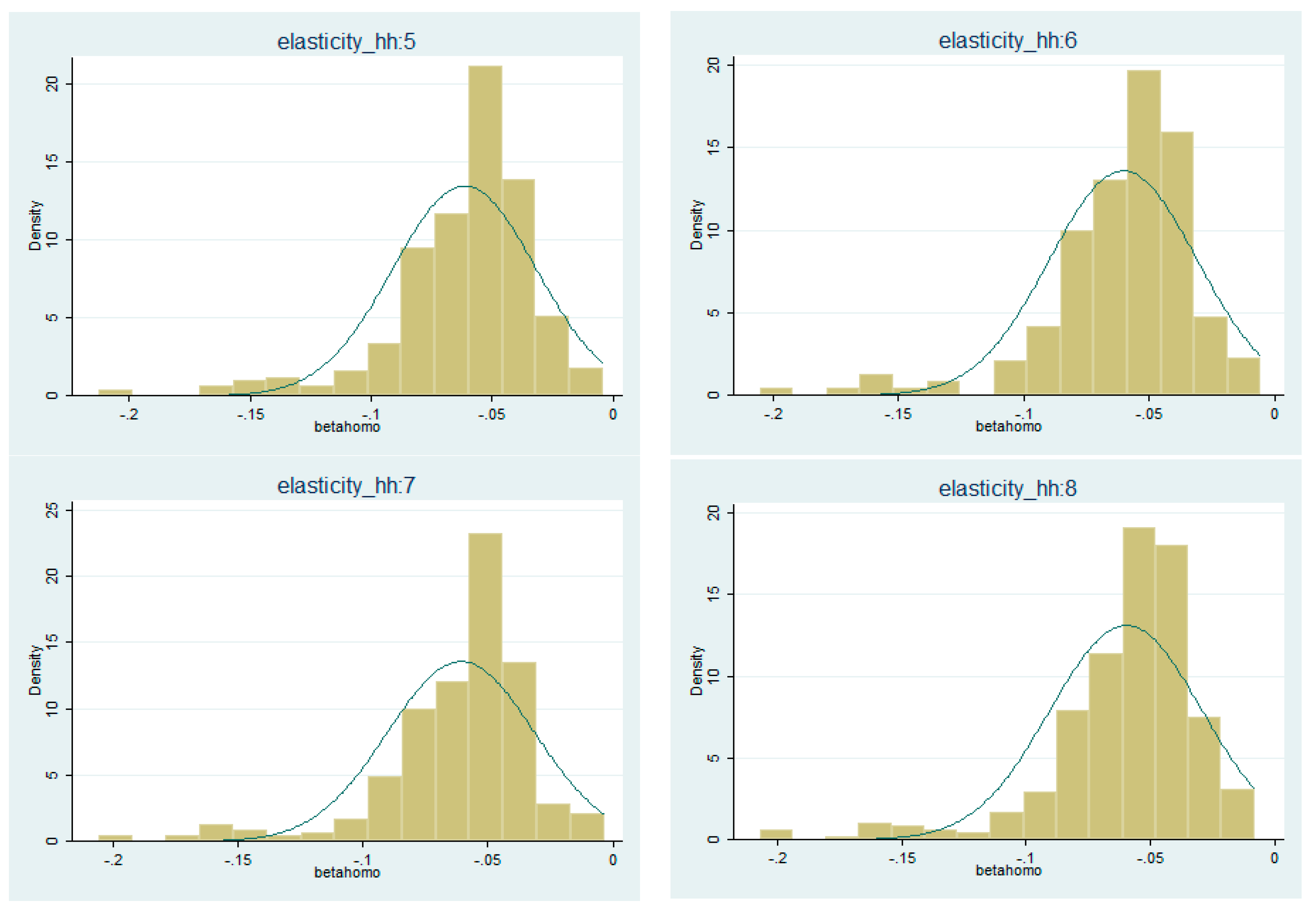
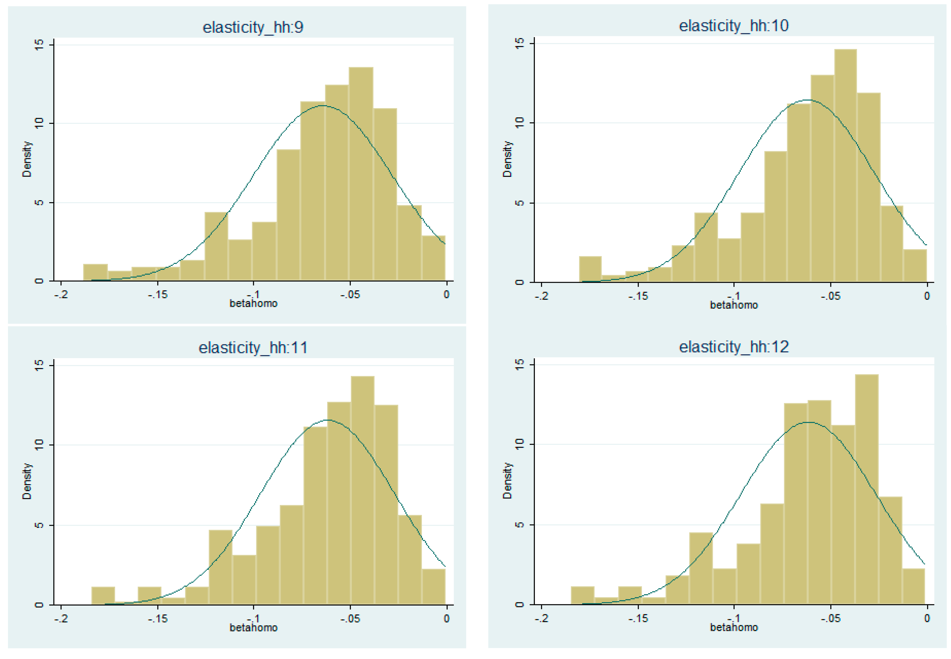
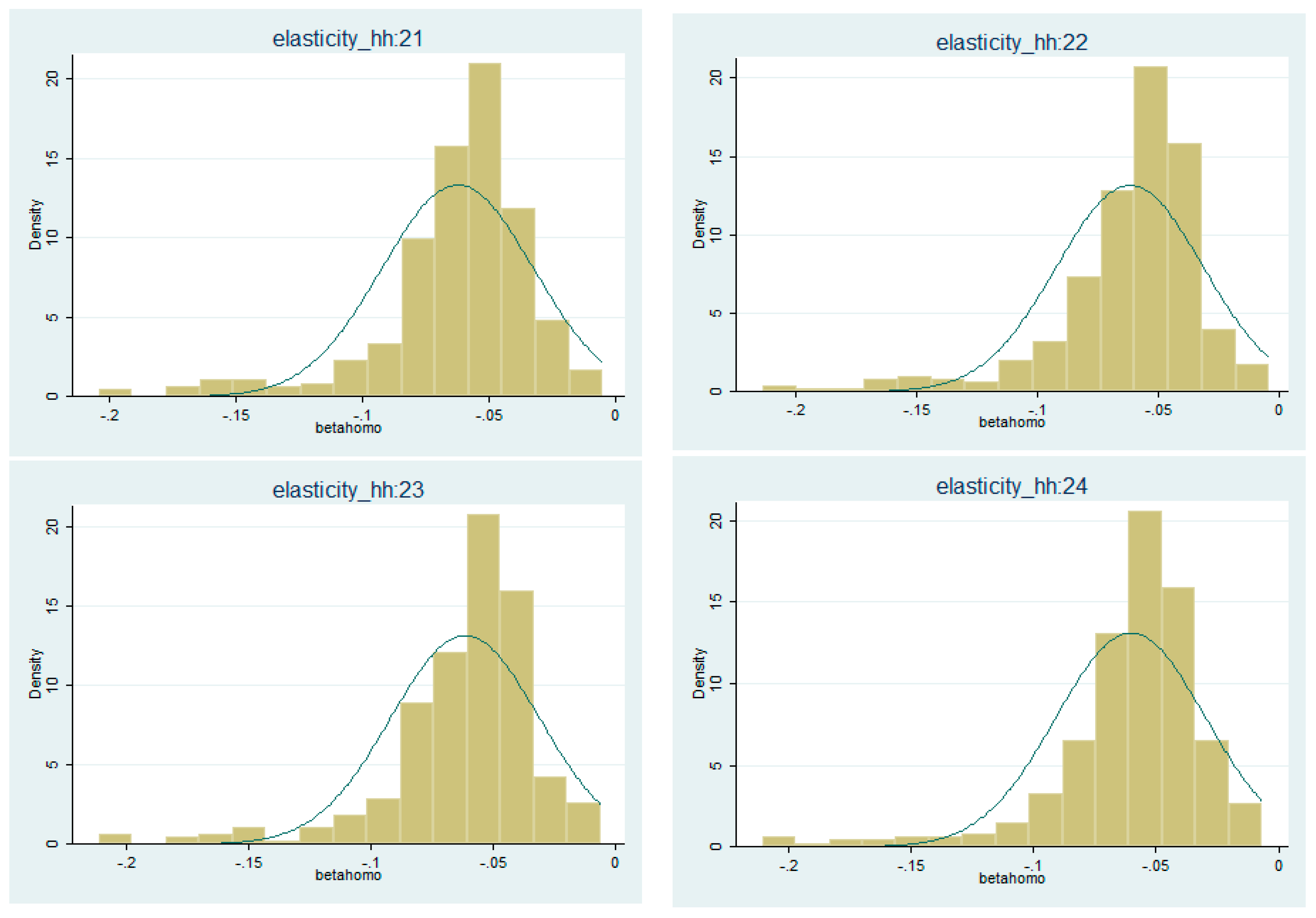
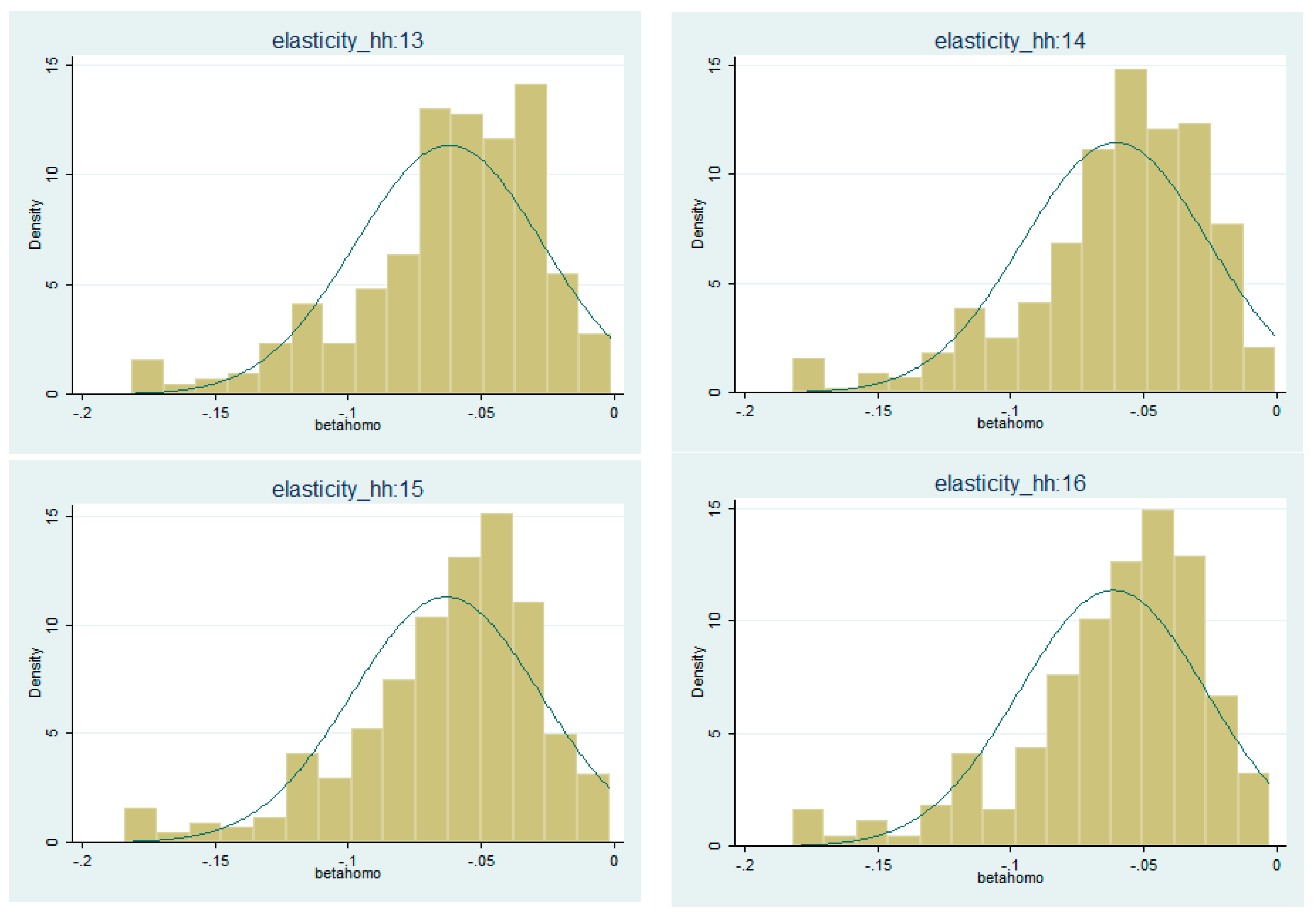
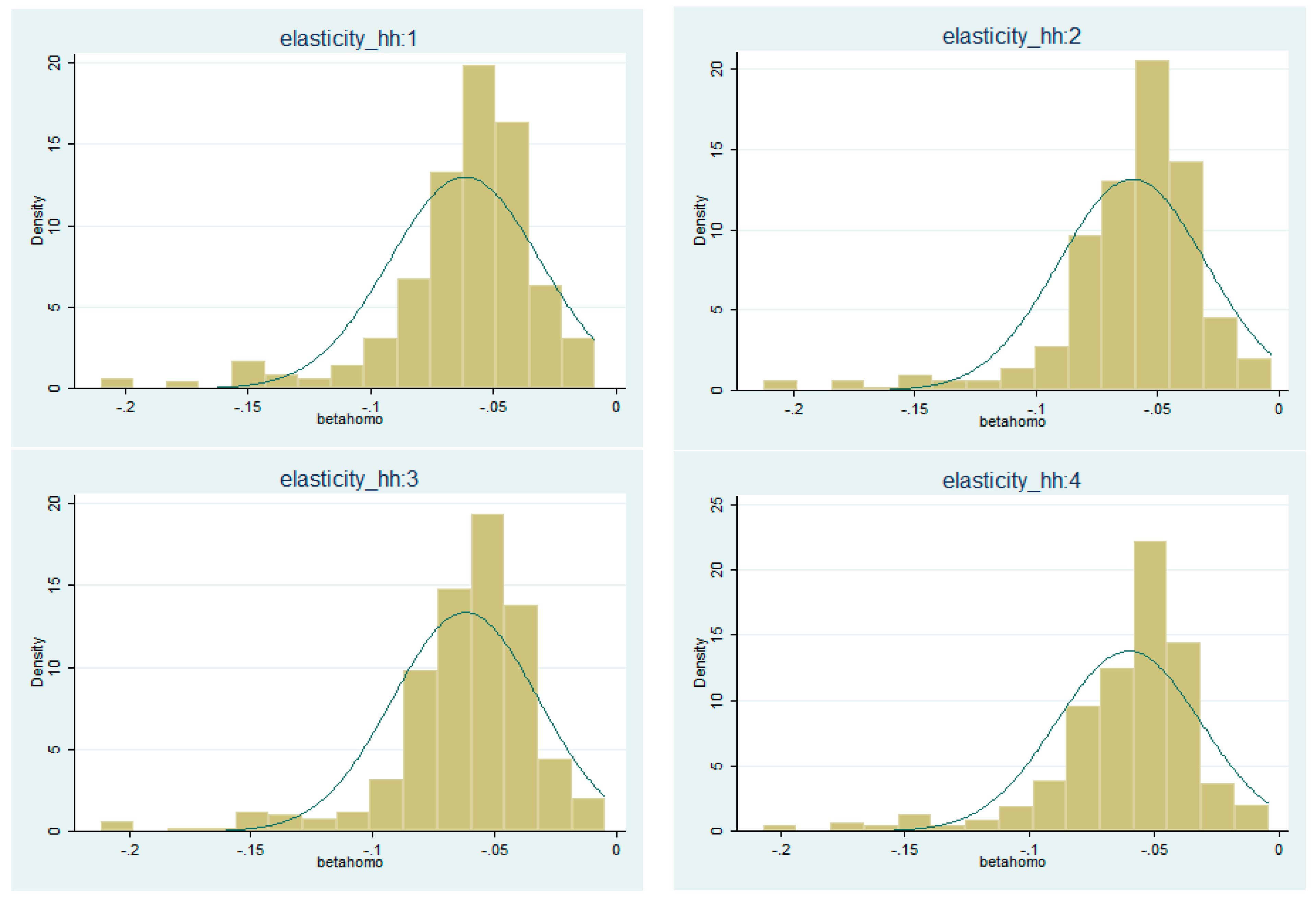
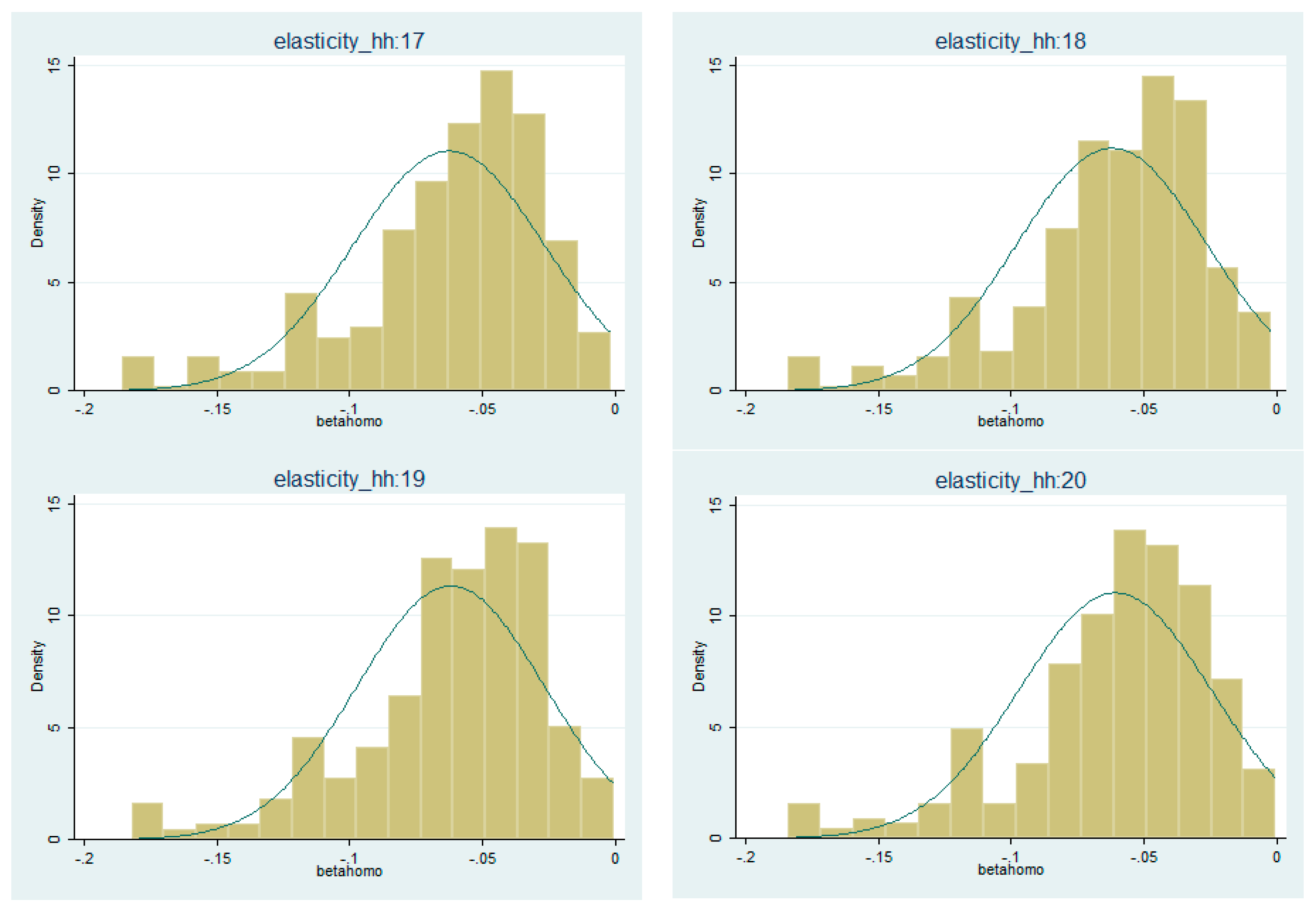
We show the elasticity distribution for each hour of the day in Figure 1, Figure 2, Figure 3, Figure 4, Figure 5 and Figure 6. On the left side we plot the distribution peak period estimates, while on the right side we plot the off-peak hour estimates. Plots graphically show that the negative skewness of off-peak estimates is greater than the peak estimates since their distributions have longer left tails.

Figure 1. Hourly elasticity distribution. 9–12 a.m.

Figure 1. Hourly elasticity distribution. 9–12 a.m.

Figure 2. Hourly elasticity distribution. 9 p.m.–0 a.m.

Figure 2. Hourly elasticity distribution. 9 p.m.–0 a.m.

Figure 3. Hourly elasticity distribution. 1–4 p.m.

Figure 3. Hourly elasticity distribution. 1–4 p.m.

Figure 4. Hourly elasticity distribution. 1–4 a.m.

Figure 4. Hourly elasticity distribution. 1–4 a.m.

Figure 5. Hourly elasticity distribution. 5–8 p.m.

Figure 5. Hourly elasticity distribution. 5–8 p.m.

Figure 6. Hourly elasticity distribution. 5–8 a.m.

Figure 6. Hourly elasticity distribution. 5–8 a.m.

4. Conclusions

In this paper, we analyzed the main features of the demand behavior in the Italian electricity market, estimating demand elasticity values, computed through Bayesian techniques. Elasticities vary within the day and around the year. Moreover, we analyzed how buyers change their load profiles within a specific group of hours given rational behavior in response to changes in prices. Since elasticity values are different from zero, buyers are reactive to change in price and their behavior is more flexible during off-peak hours. In a Bayesian framework, we can derive similar conclusions to the frequentist methods, assigning a non-informative distribution to the parameter that we want to estimate.

In our study instead, we incorporated into the model a set of prior hypothesis (influencing the inferential results) assuming that beta parameters were distributed according to a Normal distribution with negative mean (the frequentist estimate of the previous year, 2010). Starting from centered negative initial distribution, the simulation procedure leads to posteriors whose mean is higher (in absolute value) than the frequentist results. Moreover, as previously shown, the skewness of the estimates is negative in each hour of the day showing that the distributions of the elasticity values is more dispersed in the left tail. A further development of the paper could apply different model hypotheses (about the elasticities values) and compare them using Bayes factor.

The knowledge of demand elasticity values can have interesting policy implications. As is well known, the promotion of more competitive conditions in the market, insofar as it is able to shift to the right the supply function, could yield a market equilibrium, which is characterized by lower prices and higher quantities. This occurrence will have a relatively stronger effect on the equilibrium quantity, a more elastic demand curve, because the demand function will be longer. Thus, the regulator can modulate its efforts in given hours or periods of the year, according to the demand elasticity values, in order to maximize the efficiency of its policy design.

Further research should be conducted in order to investigate the advantage of using prior information to translate in quantifiable analytical terms the effect of new regulation and new policy intervention. We can incorporate into the model alternative prior distributions reflecting alternative scenarios and policy regulation. In this way, the assumption of different prior distributions (both in the functional form and in their parameters) will result in different posterior results, which would be representative of the effects of alternative policy actions.