
Optimization of a Finned Shell and Tube Heat Exchanger Using a Multi-Objective Optimization Genetic Algorithm


Abstract
:1. Introduction
2. Mathematical Modeling

| Flow regime | Regular tubes | U-tubes |
|---|---|---|
| Turbulent | 2np 1.5 | 1.6np 1.5 |
| Laminar, Re ≥ 500 | 3.25np 1.5 | 2.38np 1.5 |
3. Genetic Algorithms and Multi-Objective Optimization

4. Objective Functions
5. Case Study
| Thermophysical and process data | Tube side (water) | Shell side (oil) |
|---|---|---|
| Specific gravity (-) | 0.99 | 0.8 |
| Specific heat (J/kg K) | 4186 | 2300 |
| Dynamic viscosity (Pa s) | 0.00072 | 0.00068 |
| Thermal conductivity (W/m K) | 0.6404 | 0.1385 |
| Prandtl number (-) | 4.707 | 11.31 |
| Fouling factor (m2 W/K) | 0.000074 | 0.00015 |
| di (in) | do (in) | Dr (in) | |
|---|---|---|---|
| 1 | 0.291 | 1/2 | 0.375 |
| 2 | 0.384 | 5/8 | 0.5 |
| 3 | 0.459 | 3/4 | 0.625 |
| 4 | 0.584 | 7/8 | 0.75 |
| 5 | 0.709 | 1.0 | 0.875 |
| 6 | 0.277 | 1/2 | 0.375 |
| 7 | 0.356 | 5/8 | 0.5 |
| 8 | 0.495 | 3/4 | 0.625 |
| 9 | 0.560 | 7/8 | 0.750 |
| 10 | 0.685 | 1.0 | 0.875 |
| 11 | 0.259 | 1/2 | 0.375 |
| 12 | 0.527 | 3/4 | 0.625 |
| 13 | 0.634 | 7/8 | 0.75 |
| 14 | 0.759 | 1.0 | 0.875 |
| 15 | 0.657 | 1.0 | 0.875 |
| 16 | 0.370 | 5/8 | 0.5 |
| 17 | 0.509 | 3/4 | 0.625 |
| 18 | 0.620 | 7/8 | 0.75 |
| 19 | 0.745 | 1.0 | 0.875 |
| 20 | 0.402 | 5/8 | 0.5 |
| 21 | 0.481 | 3/4 | 0.625 |
| 22 | 0.606 | 7/8 | 0.75 |
| 23 | 0.731 | 1.0 | 0.875 |
| Variable | Lower value (or values considered) | Upper value |
|---|---|---|
| Tube arrangement | (30°, 45°, 90°) | - |
| Tube pitch rate | 1.25 | 2 |
| Tube length (m) | 3 | 8 |
| Tube number | 100 | 700 |
| Baffle spacing ratio | 0.2 | 0.4 |
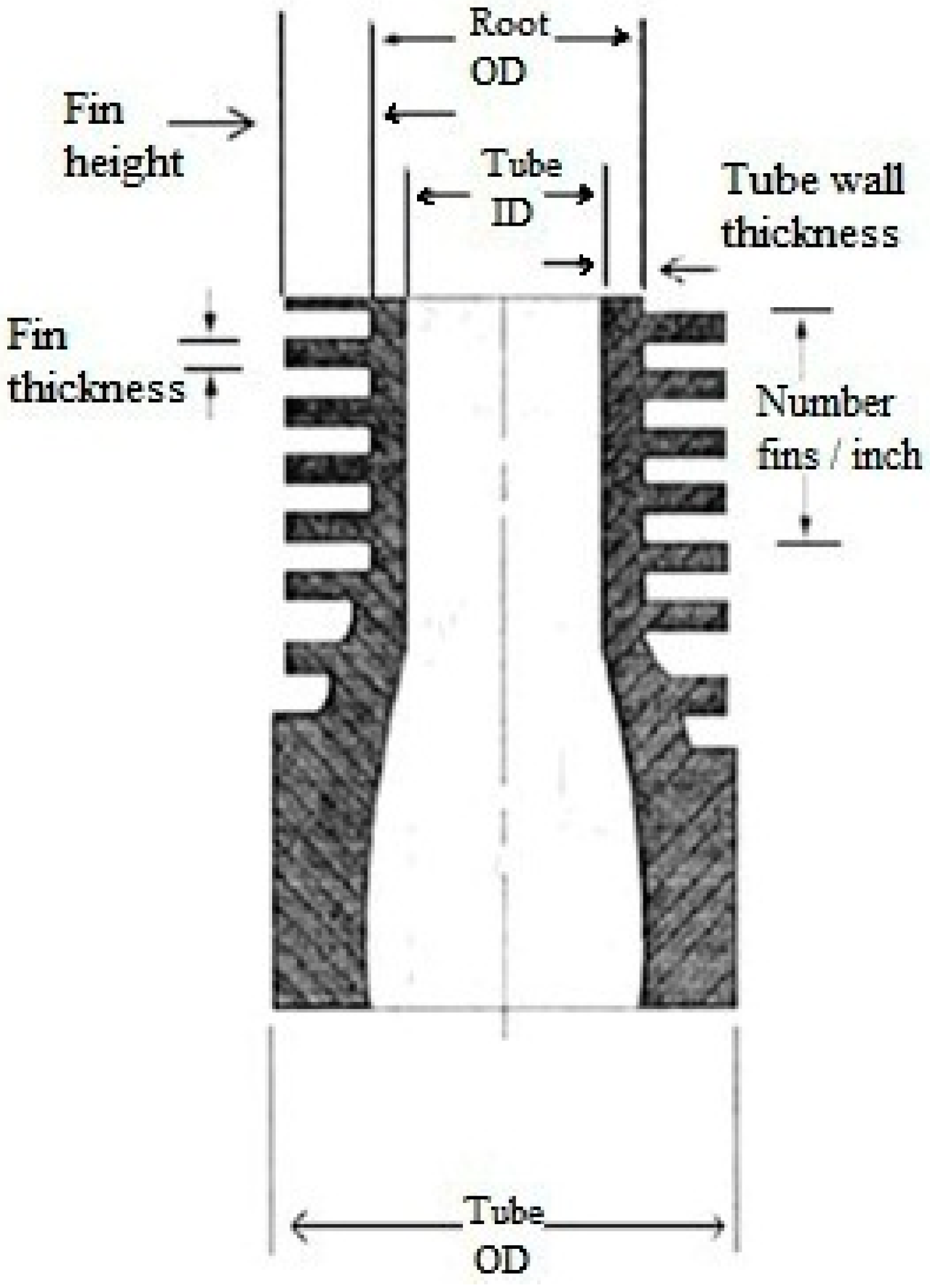
| Fin height (m) | 0.00127 | 0.003175 |
| Fin thickness (m) | 0.000254 | 0.000304 |
| Number of fins per inch length of tube | (16, 19, 26) | - |
6. Results of Optimization

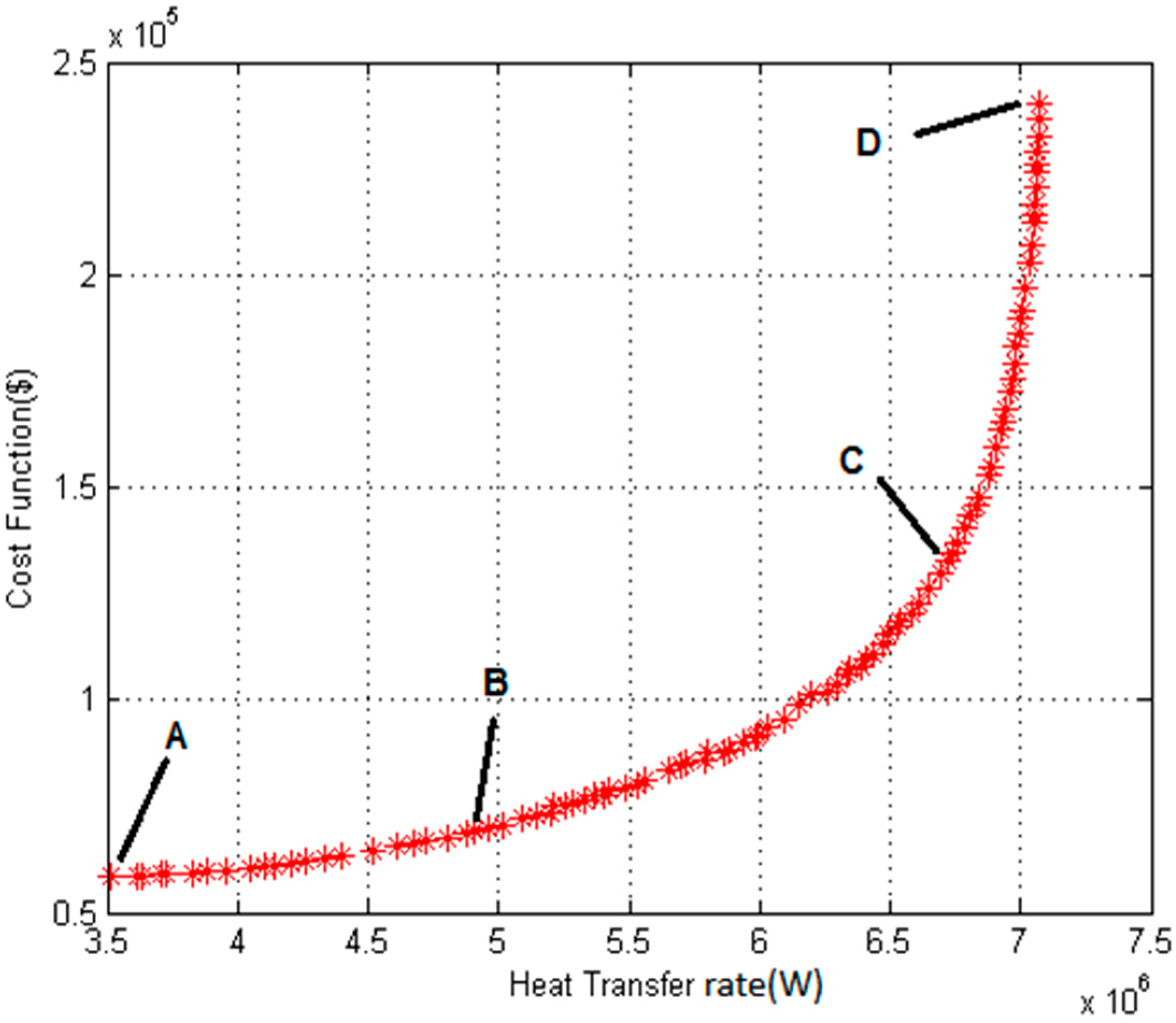
| A | B | C | D | |
|---|---|---|---|---|
| Heat transfer rate (kW) | 3517 | 4904 | 6725 | 7075 |
| Total cost ($) | 5.8 × 10⁴ | 6.9 × 10⁴ | 1.3 × 10⁵ | 2.4 × 10⁵ |
7. Conclusions
Author Contributions
Conflicts of Interest
Abbreviations
Nomenclature
| Ai | Internal surface area of tube (m2) |
| ATot | Total external surface area of a finned tube (m2) |
| As | Cross flow area at or near the shell centerline (m2) |
| B | Baffles spacing (m) |
| b | Fin height (m) |
| C | Clearance (m) |
| C* | Heat capacity rate ratio (Ch/Cmax) |
| Cin | Total investment cost ($) |
| CL | Tube layout constant (-) |
| Cmax | Maximum of Ch and Cc (W/K) |
| Cmin | Minimum of Ch and Cc (W/K) |
| Co | Annual operating cost ($/year) |
| Cop | Total operating cost ($) |
| cp | Specific heat at constant pressure (J/kg K) |
| Ctotal | Total cost ($) |
| CTP | Tube count calculation constant (-) |
| De | Equivalent diameter (m) |
| di | Tube side inside diameter (m) |
| dn | Internal diameter of nozzle (m) |
| do | Tube side outside diameter (m) |
| Dr | External diameter of tube root (m) |
| ds | Shell diameter (m) |
| f | Friction factor (-) |
| G | Mass flux (kg/m2·s) |
| H | Hours of operation per year (h/year) |
| hi | Tube side heat transfer coefficient (W/m2K) |
| ho | Shell side heat transfer coefficient (W/m2K) |
| i | Annual discount rate (%) |
| JH | Modified Colburn factor for shell-side heat transfer |
| K | Thermal conductivity (W/m K) |
| kel | Price of electrical energy ($/kWh) |
| L | Tube length (m) |
Mass flow rate (kg/s) | |
| nb | Number of baffles (-) |
| nf | Number of fins per unit length of tube (-) |
| np | Number of tube passes (-) |
| Ns | Number of shells connected in series |
| Nt | Number of tubes (-) |
| NTU | Number of transfer units (-) |
| ny | Number of baffles (-) |
| P | Pumping power (W) |
| Pr | Prandtl number (-) |
| PT | Tube pitch (m) |
| q | Heat transfer rate (W) |
| Re | Reynolds number (-) |
| RDi | Fouling resistance shell side (m2 K/W) |
| RDo | Fouling resistance shell side (m2 K/W) |
| r1 | External radius of root tube (m) |
| r2c | Corrected fin radius (m) |
| s | Fluid specific gravity (-) |
| T | Temperature (°C) |
| U | Overall heat transfer coefficient (W/m2K) |
Greek Symbols
| Ɛ | Thermal effectiveness (-) |
| ∆p | Pressure drop (Pa) |
| µ | Dynamic viscosity (Pa s) |
| Ƞ | Pump efficiency (-) |
| αr | Number of velocity heads allocated for tube-side minor pressure losses |
| τ | Fin thickness (m) |
| ρ | Density (kg/m3) |
Subscripts
| F | Fin |
| i | Inner |
| o | Outer |
| s | Shell side |
| t | Tube side |
| W | Tube wall |
References
- Şahin, A.Ş.; Kılıç, B.; Kılıç, U. Design and economic optimization of shell and tube heat exchangers using Artificial Bee Colony (ABC) algorithm. Energy Convers. Manag. 2011, 52, 3336–3346. [Google Scholar]
- Costa, A.L.H.; Queiroz, E.M. Design optimization of shell-and-tube heat exchangers. Appl. Therm. Eng. 2008, 28, 1798–1805. [Google Scholar] [CrossRef]
- Hajabdollahi, H.; Ahmadi, P.; Dincer, I. Thermo-economic optimization of a shell and tube condenser using both genetic algorithm and particle swarm. Int. J. Refrig. 2011, 34, 1066–1076. [Google Scholar] [CrossRef]
- Selbas, R.; Kızılkan, Ȍ.; Reppich, M. A new design approach for shell-and-tube heat exchangers using genetic algorithms from economic point of view. Chem. Eng. Process. 2006, 45, 268–275. [Google Scholar] [CrossRef]
- Vahdat Azad, A.; Amidpour, M. Economic optimization of shell and tube heat exchanger based on constructal theory. Energy 2011, 36, 1087–1096. [Google Scholar] [CrossRef]
- San, J.Y.; Jan, C.L. Second-law analysis of a wet cross flow heat exchanger. Energy 2000, 25, 939–955. [Google Scholar] [CrossRef]
- Gupta, A.; Das, S.K. Second law analysis of cross flow heat exchanger in the presence of axial dispersion in one fluid. Energy 2007, 32, 664–672. [Google Scholar] [CrossRef]
- Satapathy, A.K. Thermodynamic optimization of a coiled tube heat exchanger under constant wall heat flux condition. Energy 2009, 34, 1122–1126. [Google Scholar] [CrossRef]
- Sanaye, S.; Hajabdollahi, H. Thermal-economic multi-objective optimization of plate fin heat exchanger using genetic algorithm. Appl. Energy 2009, 87, 1893–1902. [Google Scholar] [CrossRef]
- Najafi, H.; Najafi, B.; Hoseinpoori, P. Energy and cost optimization of a plate and fin heat exchanger using genetic algorithm. Appl. Therm. Eng. 2011, 31, 1839–1847. [Google Scholar] [CrossRef]
- Hajabdollahi, H.; Tahani, M.; ShojaeeFard, M.H. CFD modeling and multi-objective optimization of compact heat exchanger using CAN method. Appl. Therm. Eng. 2011, 31, 2597–2604. [Google Scholar] [CrossRef]
- Sanaye, S.; Hajabdollahi, H. Multi-objective optimization of shell and tube heat exchangers. Appl. Therm. Eng. 2010, 30, 1937–1945. [Google Scholar] [CrossRef]
- Hilbert, R.; Janiga, G.; Baron, R.; Thevenin, D. Multi-objective shape optimization of a heat exchanger using parallel genetic algorithms. Int. J. Heat Mass Transf. 2006, 49, 2567–2577. [Google Scholar] [CrossRef]
- Fettaka, S.; Thibault, J.; Gupta, Y. Design of shell-and-tube heat exchangers using multi-objective optimization. Int. J. Heat Mass Transf. 2013, 60, 343–354. [Google Scholar] [CrossRef]
- Ponce, J.M.; Serna, M.; Rico, V.; Jimenez, A. Optimal design of shell-and-tube heat exchangers using genetic algorithms. Comput. Aided Chem. Eng. 2006, 21, 985–990. [Google Scholar]
- Mizutani, F.T.; Pessoa, F.L.P.; Queiroz, E.M.; Grossmann, S. Mathematical programming model for heat exchanger network synthesis including detailed heat exchanger designs. Ind. Eng. Chem. Res. 2003, 42, 4009–4018. [Google Scholar] [CrossRef]
- Babu, B.V.; Munawar, S.A. Differential evolution for the optimal design of heat exchangers. Chem. Eng. Sci. 2007, 62, 3720–3739. [Google Scholar] [CrossRef]
- Caputo, A.C.; Pelagagge, P.M.; Salini, P. Heat exchanger design based on economic optimization. Appl. Therm. Eng. 2008, 28, 1151–1159. [Google Scholar] [CrossRef]
- Shah, R.K.; Sekulic, P. Fundamental of Heat Exchanger Design; John Wiley & Sons: New York, NY, USA, 2003. [Google Scholar]
- Kakac, S.; Liu, H. Heat Exchangers Selection Rating, and Thermal Design; CRC Press: New York, NY, USA, 2000. [Google Scholar]
- All Free Industrial Ebooks (IE) and Software Downloads. Industrial Training, Mechanical: Heat Exchanger Training. Available online: http://www.industrial-ebooks.com/ (accessed on 3 October 2013).
- Serth, R.W. Process Heat Transfer Principles and Applications; Academic Press: Kingsville, TX, USA, 2007. [Google Scholar]
- McQuiston, F.C.; Tree, D.R. Optimum space envelopes of the finned tube heat transfer surface. Trans. ASHRAE 1972, 78, 144–152. [Google Scholar]
- Seider, E.N.; Tate, C.E. Heat transfer and pressure drop of liquids in tubes. Ind. Eng. Chem. 1936, 28, 1429–1435. [Google Scholar] [CrossRef]
- Kern, D.Q.; Krause, A.D. Extended Surface Heat Transfer; McGraw-Hill: New York, NY, USA, 1972. [Google Scholar]
- Hausen, H. Darstellung des warmeuberganges in Rohrendurch Verallgemeinerte Potenziehungen. Z.VDI Beih Verfahrenstech 1943, 4, 91–98. [Google Scholar]
- Kern, D.Q. Process Heat Transfer; McGraw-Hill: New York, NY, USA, 1950. [Google Scholar]
- Henry, J.A.R. Headers, Nozzles and Turnarounds, in Heat Exchanger Design Handbook; Hemisphere Publishing Corporation: New York, NY, USA, 1988; Volume 2. [Google Scholar]
- Taborek, J. Industrial heat exchanger design practices. In Boiler Evaporators, and Condenser; John Wiley & Sons: New York, NY, USA, 1991. [Google Scholar]
- Rechenberg, I. Evolutionsstrategie: Optimierung Technischer Systeme Nach Prinzipien der Biologischen Evolution; Formmann-Holzboog Verlag: Stuttgart, Germany, 1973. [Google Scholar]
- Holland, J.H. Adaptation in Natural and Artificial Systems; MIT Press: Cambridge, MA, USA, 1992. [Google Scholar]
- Goldberg, D.E. Genetic Algorithms in Search, Optimization, and Machine Learning; Addison-Wesley: Berkshire, UK, 1989. [Google Scholar]
- Srinivas, N.; Deb, K. Multi-objective optimization using non-dominated sorting in genetic algorithms. J. Evol. Comput. 1994, 2, 221–248. [Google Scholar] [CrossRef]
- Deb, K.; Agrawal, S.; Pratab, A.; Meyarivan, T. A fast elitist none-dominated sorting in genetic algorithm for multi-objective optimization: NSGA-II. In Proceedings of the Parallel Problem Solving from Natural PPSN VI, Paris, France, 18–20 September 2000.
- Deb, K.; Pratap, A.; Sameer, A.; Meyarivan, T. A fast elitist multi-objective genetic algorithm: NSGA-II. IEEE Trans. Evolut. Comput. 2008, 6, 182–197. [Google Scholar] [CrossRef]
- Taal, M.; Bulatov, I.; Klemes, J.; Stehlik, P. Cost estimation and energy price forecasts for economic evaluation of retrofit projects. Appl. Therm. Eng. 2003, 23, 1819–1835. [Google Scholar] [CrossRef]
© 2015 by the authors; licensee MDPI, Basel, Switzerland. This article is an open access article distributed under the terms and conditions of the Creative Commons Attribution license (http://creativecommons.org/licenses/by/4.0/).
Share and Cite
Sadeghzadeh, H.; Aliehyaei, M.; Rosen, M.A. Optimization of a Finned Shell and Tube Heat Exchanger Using a Multi-Objective Optimization Genetic Algorithm. Sustainability 2015, 7, 11679-11695. https://doi.org/10.3390/su70911679
Sadeghzadeh H, Aliehyaei M, Rosen MA. Optimization of a Finned Shell and Tube Heat Exchanger Using a Multi-Objective Optimization Genetic Algorithm. Sustainability. 2015; 7(9):11679-11695. https://doi.org/10.3390/su70911679
Chicago/Turabian StyleSadeghzadeh, Heidar, Mehdi Aliehyaei, and Marc A. Rosen. 2015. "Optimization of a Finned Shell and Tube Heat Exchanger Using a Multi-Objective Optimization Genetic Algorithm" Sustainability 7, no. 9: 11679-11695. https://doi.org/10.3390/su70911679