Optimization of the Waterbus Operation Plan Considering Carbon Emissions: The Case of Zhoushan City

Abstract

Recently, as more people are concerned with the issues around environment protection, research about how to reduce carbon emissions has drawn increasing attention. Encouraging public transportation is an effective measure to reduce carbon emissions. However, overland public transportation does less to lower carbon because of the gradually increasing pressure of the urban road traffic. Therefore, the waterbus along the coast becomes a new direction of the urban public transport development. In order to optimize the operation plan of the waterbus, a bi-level model considering carbon emissions is proposed in this paper. In the upper-level model, a multiple objective model is established, which considers both the interests of the passengers and the operator while considering the carbon emissions. The lower-level model is a traffic model split by using a Nested Logit model. A NSGA-II (Non-dominated Sorting Genetic Algorithm-II) algorithm is proposed to solve the model. Finally, the city of Zhoushan is chosen as an example to prove the feasibility of the model and the algorithm. The result shows that the proposed model for waterbus operation optimization can efficiently reduce transportation carbon emissions and satisfy passenger demand at the same time.

1. Introduction

Climate change resulting from the emission of carbon dioxide associated with human economic activities has the potential to create an unstable global climatic future [1]. Nowadays, carbon emission has become a global issue. According to the IEA (International Energy Agency), 23% of the global energy-related carbon emission comes from the transport sector [2]. Additionally, that figure will grow to 41% by 2030 [3]. Vehicles are the biggest carbon emitter in urban traffic. A study by Barth [4] has shown that carbon emissions of vehicles are the highest in cases of stop-and-go traffic and high-speed situations. It is clear that when road congestion occurs, all the vehicles will be in a stop-and-go situation, and the carbon emissions of vehicles will be higher accordingly. However, developing waterbuses in coastal and riverside cities can both alleviate road pressure and reduce the carbon emissions of the transport sector. Furthermore, the waterbus needs little investment because it can operate using existing water resources without building roads. In addition, though the waterbus has opened in some cities, the poor level of waterbus service due to bad arrangements leads to declining traffic. Therefore, the existing waterbus cannot compete with overland transport to share the traffic of vehicles.

Because of the reasons above, this paper proposes an optimization of the waterbus operation plan in terms of carbon emissions. Part of overland traffic is transferred to the waterbus by improving the waterbus service level, which can alleviate the road pressure and reduce the carbon emissions of the transport sector. However, massive expenditures need to be spent to improve the waterbus service level. In order to improve the feasibility of the waterbus operation plan, the toll revenue of the road is used to subsidize the waterbus in order to alleviate the pressure of funding. At the same time, raising the traffic tolls increases the trip cost of cars and somewhat curbs the usage of cars, therefore encouraging people to make greater use of the waterbus. Thus, the target to cut emissions of the transport sector would be reached by the above method.

Compared with the optimization of overland bus operation plans, the waterbus is much simpler because of its smaller site scale and lack of interference from other transportation modes. Furthermore, unlike the road, the sea in which waterbuses sail has no capacity limitations [5]. However, on account of the narrow application range of the waterbus (limited to coastal and riverside cities), there are few studies about the waterbus. Ye et al. [6] used a disaggregate model to analyze the attractiveness of the waterbus with Shanghai and Huai’an as examples. Sato and Takadama [7] studied the waterbus line planning problem using a Pittsburgh-style learning classifier system (LCS) and researched a way that ensured the robustness of the waterbus system to make the waterbus continue to serve passengers even in bad weather. Li and Huang [8] studied the characteristics of Guangzhou waterbus passengers based on IC (Integrated Circuit) cards, and they drew a conclusion that the waterbus is more attractive to non-commuters than commuters. Keiki and Keiji [9] studied the classifier system for multiple environments: towards a robust waterbus route for several situations, and in the same year, he found a new method to optimize the waterbus route through the Pittsburgh-style learning classifier system [10].

The study of the overland bus is more sophisticated than the waterbus, so it can be a reference for the study of the waterbus. Ortuzar and Willumson [11] presented the most important transport modeling techniques and they have approached the subject from the point of view of a modeling exercise, discussing the role of theory, data, model specification in its widest sense, model estimation, validation, and forecasting. Cascetta [12] provided a comprehensive and systematic presentation of the mathematical models for the simulation of transportation systems. Methodologies for the analysis and design of these systems were provided as well. Lam and Bell [13] addressed the current problem of improving public transit systems by taking advantage of new technologies and advanced modeling techniques. The key areas open to improvement were service planning and operations management. Russo et al. [14] estimated the target time of trucks that transport agriculture and food products subject to commercial and production constraints. Vitetta et al. [15] investigated the shortcomings of the frequency approach using optimal strategy compared with the schedule-based approach in simulating ex-urban transit systems in terms of user behavior simulation and subsequently verifying a numerical application. Bloom and Mathew [16] thought that the main emphasis of bus transit route network optimization was bus routes and schedules. The passenger demand was satisfied and the cost of the bus company was minimized by optimizing bus routes and schedules. Dubois et al. [17] optimized a bus transit route network considering factors such as geography, capacity, direct demands, and transfers. Baaj and Mahmassani [18] designed a route-generation algorithm (RCA) to optimize bus lines and frequency. Agrawal and Mathew [19] set up an optimization model of a bus transit route network, in which the objective was to minimize the transportation costs, and calculated the model with the genetic algorithm (GA). Yu et al. [20] proposed models to predict bus arrival times at the same bus stop but with different routes and several methods, which included support vector machine (SVM), artificial neural network (ANN), k nearest neighbors algorithm (k-NN), and linear regression (LR). Shih [21] and Chakroborty et al. [22] proposed the optimization models to optimize the fleet size distribution and scheduling. Cordeau [23] presented recent optimization models for the most commonly studied rail transportation problems, which concentrated on routing and scheduling problems. Similar research problems have been studied by Chakroborty [24], Yao et al. [25,26], and Yu et al. [27].

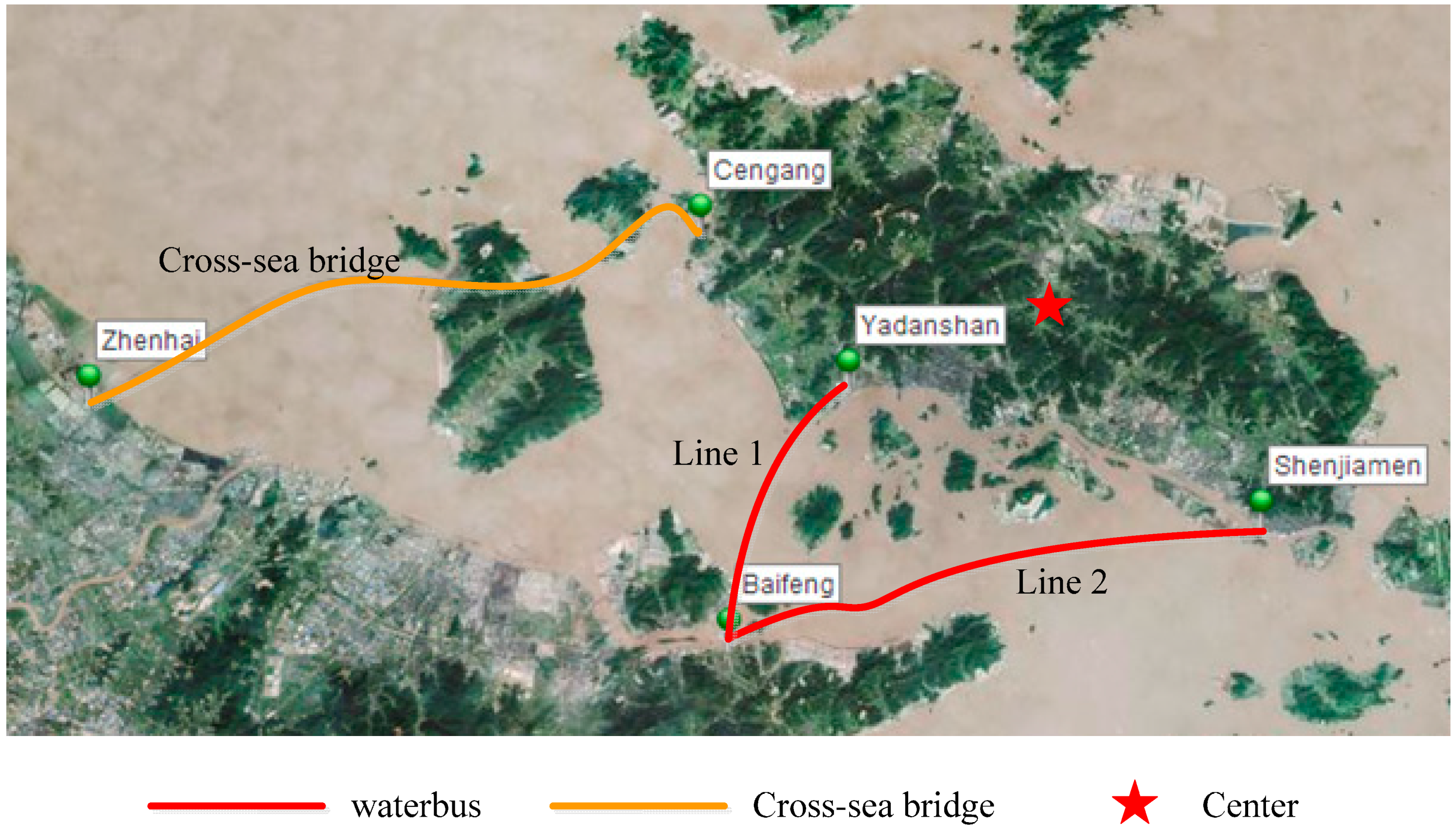
Referring to existing research and studies, this paper studied the waterbus operation plan problem in three aspects: environment, passengers, and waterbus operators. A bi-level model is proposed in this paper. In the upper-level model, a multiple objective model is established, which considers the benefits of both the passengers and the operator while considering the carbon emissions. The lower-level model is a traffic model split by using a Nested Logit model. After calculation, we expect to find a balance point among passenger demand, a low cost for the operators, and low carbon emissions of the transport sector. Finally, the trip between Zhoushan and Ningbo cities is chosen as an example to test the model.

This paper is organized as follows: the second section describes the problems and introduces the background of the city of Zhoushan. A bi-level model is proposed in the third section. The fourth section introduces the NSGA-II algorithm and, in the fifth part, the city of Zhoushan is chosen as a setting to test the model. The conclusion can be found in the last part.

2. Problem Description and Background

2.1. Problem Description

As is shown in Figure 1, there is both road-based and marine transportation between the cities of Zhoushan and Ningbo. People can drive across the cross-sea bridge or take the waterbus, which includes two types of ships, the passenger ship and the ro-ro passenger ship. This paper aims at transferring part of the overland traffic to the waterbus by improving the waterbus service level. The transfer traffic can alleviate the road pressure and reduce the carbon emissions of the transport sector. However, massive expenditures need to be spent to improve the waterbus service level. In order to improve the feasibility of the waterbus operation plan, the toll revenue of the cross-sea bridge is used to subsidize the waterbus to alleviate the pressure of funding. At the same time, raising the traffic tolls increases the trip cost of cars and somewhat curbs the usage of cars, which encourages people to make greater use of the waterbus. Due to the improvement of the waterbus service level and the rising toll of the cross-sea bridge, an increasing number of people enjoy traveling by waterbus while fewer people drive across the cross-sea bridge. It is expected to strike a balance between the waterbus and the cross-sea bridge which meet the passenger demand, provide a low cost for the operators, and lower the carbon emissions of the transport sector.

Figure 1. Trip modes of people.

Figure 1. Trip modes of people.

2.2. Background

The city of Zhoushan is located on an archipelago in China, which has 1390 islands and reefs. Therefore, Zhoushan is known as “the city of a thousand islands”. Zhoushan Island, with an area of 502 square kilometers, is the biggest island in the city of Zhoushan. The permanent population of Zhoushan Island is 700,000, which accounts for 62.5 percent of the population of Zhoushan. The city of Ningbo is one of the most important cities that connect Zhoushan with the outside world. As Figure 2 shows, there are two waterbus lines between Ningbo and Zhoushan Island proper: the Baifeng passenger terminal of Ningbo to Yadanshan passenger terminal of Zhoushan Island is Line 1; the Baifeng passenger terminal of Ningbo to Shenjiamen passenger terminal of Zhoushan Island is Line 2. Additionally, there is also a cross-sea bridge connecting Ningbo to Zhoushan Island.

The data of this paper comes from the survey undertaken in Zhoushan via Dalian Maritime University in September 2012. According to the survey, origin-destination (OD) traffic volume was 33,928 from Ningbo to Zhoushan Island, in which there were 15,448 cars across the cross-sea bridge. Saturation of the cross-sea bridge was about 0.7. The average saturation of the expressway is 0.4, so the traffic congestion occurred on the cross-sea bridge. The service capacity of the cross-sea bridge cannot meet traffic demands as vehicle ownership continues to increase. Although the waterbus has opened between Ningbo and Zhoushan Island, the waterbus lost its attraction to passengers due to the poor service level. Therefore, the existing waterbus between Ningbo and Zhoushan Island cannot compete with the cross-sea bridge to share the traffic of vehicles.

There are two kinds of people traveling between Ningbo and Zhoushan Island. The first are local residents who work or study in Ningbo, and the trip modes of these people are taking the waterbus (Line 1 and Line 2) and driving across the cross-sea bridge. The other people are tourists who travel to the Putuo District of Zhoushan Island, and they usually drive across the cross-sea bridge or take the waterbus (Line 2). This paper studies the waterbus operation plans of Line 1 and Line 2. As most people tour on the non-workday, the waterbus operation plan of Line 2 is optimized on the workday and non-workday, respectively.

Figure 2. Trip lines between Ningbo and Zhoushan Island.

Figure 2. Trip lines between Ningbo and Zhoushan Island.

3. Optimization Model for the Waterbus Operation Plan

A bi-level model is proposed in this paper. The upper-level model is a multiple objective model [28], and the decision variables are the numbers of waterbuses, the departure frequency, and the fares. Objective equation 1 is the minimum of the total trip costs of passengers. Objective equation 2 is the minimum of the operation costs of operators. Minimizing the carbon emission costs of both waterbuses and cars on the cross-sea bridge is objective equation 3. The lower-level model is a traffic model split by using a Nested Logit model [29]. The attributes under examination are the trip time costs and fares associated with each available mode. We first present a formal definition of the problem. Please see Table 1 for a summary of the notation used in this paper.

Table 1. Table of notations.

Description	Notation
Ship types of the waterbus	$i$
$i=1$ denotes passenger ship
$i=2$ denotes ro-ro passenger ship (for people)
$i=3$ denotes ro-ro passenger ship (for cars)
The line between Ningbo and Zhoushan	$k$
Average running speed of waterbus	$v_i^w$
Waterbus distance traveled through line $k$	$s_{ik}^w$
Cross-sea bridge distance traveled through line $k$	$s_k^c$
Waterbus wait time of passengers through line $k$	$T_{ik}^w$
Unit time cost	$d^t$
Fares of the three kinds of waterbus through line $k$	$C_{ik}^w$
Cross-sea bridge toll of each car through line $k$	$C_k^c$
Penalty cost	$C_{punish}$
Number of passengers of waterbus through line $k$	$q_{ik}^w$
Number of people across cross-sea bridge through line $k$	$q_k^c$
Average running speed of cars	$v^c$
Number of people across cross-sea bridge through line $k$	$q_k^c$
Conversion coefficient for the cars	$\text{μ}$
Unit fuel consumption of cars	$Q^c$
Unit cost of gasoline	$d^c$
Base period of the calculation	$T$
Departure frequency of waterbus of line $k$	$f_{ik}^w$
Number of waterbuses on line $k$	$n_{ik}^w$
Travel distance of passengers through line $k$	$S_k$
Fare of taxi taken by passenger after going ashore from the waterbus	$C^T$
Depreciation of waterbus	$D_i^w$
Fuel consumption of waterbus per day	$Q_i^w$
Unit cost of fuel	$d^b$
Carbon emissions of waterbus on line $k$	$E{Q}_{ik}^w$
Carbon emission coefficient for waterbus or cars	$E{q}^w$, $E{q}^c$
Conversion coefficient of emission cost	$\text{ε}$
Traffic assignment of cross-sea bridge or waterbus of line $k$	$P_k^c$, $P_k^w$
Traffic assignment of the three kinds of waterbus of line $k$	$P_{ik}^w$
Utilities of waterbus or cross-sea bridge of line $k$	$V_k^w$, $V_k^c$
Utilities of three kinds of waterbus of line $k$	$V_{ik}^w$
Traveling time costs of the three kinds of waterbus of line $k$	$c_{ik}^w$
Traveling time costs of cross-sea bridge	$c_k^c$
Capacity limit of each kind of waterbus	$E_i$

Table 1. Table of notations.

Description	Notation
Ship types of the waterbus	$i$
$i=1$ denotes passenger ship
$i=2$ denotes ro-ro passenger ship (for people)
$i=3$ denotes ro-ro passenger ship (for cars)
The line between Ningbo and Zhoushan	$k$
Average running speed of waterbus	$v_i^w$
Waterbus distance traveled through line $k$	$s_{ik}^w$
Cross-sea bridge distance traveled through line $k$	$s_k^c$
Waterbus wait time of passengers through line $k$	$T_{ik}^w$
Unit time cost	$d^t$
Fares of the three kinds of waterbus through line $k$	$C_{ik}^w$
Cross-sea bridge toll of each car through line $k$	$C_k^c$
Penalty cost	$C_{punish}$
Number of passengers of waterbus through line $k$	$q_{ik}^w$
Number of people across cross-sea bridge through line $k$	$q_k^c$
Average running speed of cars	$v^c$
Number of people across cross-sea bridge through line $k$	$q_k^c$
Conversion coefficient for the cars	$\text{μ}$
Unit fuel consumption of cars	$Q^c$
Unit cost of gasoline	$d^c$
Base period of the calculation	$T$
Departure frequency of waterbus of line $k$	$f_{ik}^w$
Number of waterbuses on line $k$	$n_{ik}^w$
Travel distance of passengers through line $k$	$S_k$
Fare of taxi taken by passenger after going ashore from the waterbus	$C^T$
Depreciation of waterbus	$D_i^w$
Fuel consumption of waterbus per day	$Q_i^w$
Unit cost of fuel	$d^b$
Carbon emissions of waterbus on line $k$	$E{Q}_{ik}^w$
Carbon emission coefficient for waterbus or cars	$E{q}^w$, $E{q}^c$
Conversion coefficient of emission cost	$\text{ε}$
Traffic assignment of cross-sea bridge or waterbus of line $k$	$P_k^c$, $P_k^w$
Traffic assignment of the three kinds of waterbus of line $k$	$P_{ik}^w$
Utilities of waterbus or cross-sea bridge of line $k$	$V_k^w$, $V_k^c$
Utilities of three kinds of waterbus of line $k$	$V_{ik}^w$
Traveling time costs of the three kinds of waterbus of line $k$	$c_{ik}^w$
Traveling time costs of cross-sea bridge	$c_k^c$
Capacity limit of each kind of waterbus	$E_i$

3.1. Upper-Level Model

Objective Equation (1):

$$\begin{array}{cc}\min & {\displaystyle \sum _k\{{\displaystyle \sum _{i=1}^3\left[\left(\frac{s_{ik}^w}{v_i^w}+T_{ik}^w\right)\times d^t+C_{ik}^w+C_{punish}\right]\times q_{ik}^w}}\end{array}+\left(\frac{s_k^c}{v^c}\times d^t\times q_k^c+C_k^c\times \frac{q_k^c}{\text{μ}}+s_k^c\times Q^c\times d^c\right)\}\times T$$

(1)

where $d^t$ is the unit time cost. As the values of $d^t$ and emission costs are difficult to measure and it is also time-consuming to measure unit time cost and emission cost, we referred to the paper of Yu et al. [30]. μ is the conversion coefficient for the cars. μ is 1.5 in this paper, which denotes that the average people in a car is 1.5; and T represents the base period of the calculation. In this paper, one year is the base period.

$$T_{ik}^w=\frac{1}{2}\times f_{ik}^w$$

(1a)

$$f_{ik}^w=\frac{s_{ik}^w\times 2}{v^w\times n_{ik}^w}$$

(1b)

$$C_{punish}=\frac{S_k}{v^c}\times d^t+C^T$$

(1c)

The penalty cost is considered because passengers should transfer over land traffic modes to go to the destination after going ashore from the waterbus. This paper assumes that passengers take a taxi to go to the destination.

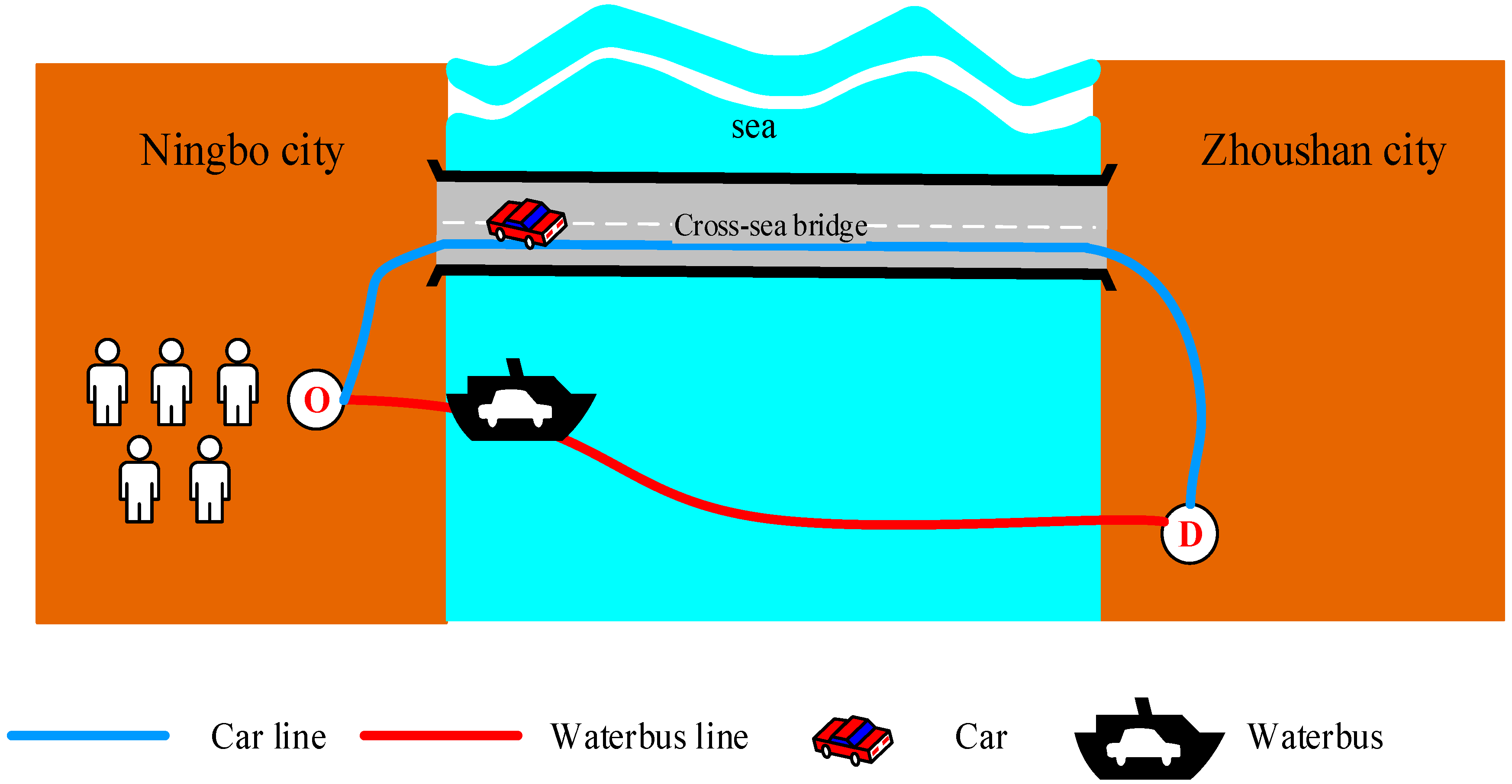
The objective Equation (1) is the minimum of the total travel cost of people. The first part of the equation is the travel costs of passengers who take the waterbus, which consists of the waterbus traveling time cost (waterbus traveling time cost and the passengers’ waiting time cost), the fares of the waterbus, and the fares of taxi. There are parking lots and riding facilities in the passenger terminals of the waterbuses. If passengers go to the terminal by car and do not want to take the ro-ro passenger ship, they can park in the parking lot. After these passengers go ashore, they can use other modes of transportation, such as taxis, buses, and so on. If passengers drive to the terminal and want to arrive at the destination in their cars, they can take the ro-ro passenger ship. The second part of the equation is the travel costs of people who drive across the cross-sea bridge, which consists of the traveling time cost (drive), the toll of the cross-sea bridge, and the costs of fuel.

Objective Equation (2):

$$\begin{array}{cc}\min & {\displaystyle \sum _k\left[{\displaystyle \sum _{i=1}^3\left(D_i^w\times n_{ik}^w+Q_i^w\times s_{ik}^w\times d^b\right)}-\frac{1}{2}\times C_k^c\times \frac{q_k^c}{\text{μ}}\right]}\end{array}\times T$$

(2)

The objective Equation (2) is the minimum of the operation cost of the operator, which consists of the depreciation of the waterbus and the cost of fuel consumption minus the subsidy from the toll revenue of the cross-sea bridge.

Objective Equation (3):

$$\begin{array}{cc}\min & {\displaystyle \sum _k\left({\displaystyle \sum _{i=1}^3\left(E{Q}_{ik}^w\times n_{ik}^w+S_k\times E{q}^c\times \frac{q_{ik}^w}{\text{μ}}\right)}+S_k^c\times E{q}_k^c\times \frac{q_k^c}{\mu }\right)}\times \epsilon \end{array}\times T$$

(3)

$$E{Q}_{ik}^w=S_{ik}^w\times Q^w\times E{q}^w\times {10}^3$$

(3a)

$$E{q}^c=\frac{{\eta }_1}{v^c}+{\eta }_2\times v^c+{\eta }_3\times {\left(v^c\right)}^2+{\eta }_4$$

(3b)

According to IPCC (Intergovernmental Panel on Climate Change), the value of $E{q}^w$ is 3.17 tons of carbon dioxide generated by one ton of fuel [31]. $E{q}^c$ is a equation of the speed [32], where ${\text{η}}_1$, ${\text{η}}_2$, ${\text{η}}_3$, ${\text{η}}_4$ are constant terms and ε is the conversion coefficient of the emission cost.

The objective Equation (3) is the minimum of the carbon emission cost, which includes the carbon emission cost of passengers taking the waterbus and people driving across the cross-sea bridge. Additionally, the carbon emission cost of passengers is made up of the waterbus carbon emission cost and the taxi carbon emission cost.

3.2. Lower-Level Model

When choosing travel modes, passengers are usually affected by many factors, such as traveling time, cost, security, and comfort. After weighing all the influence factors, passengers will select the most advantageous mode for their own travel [33]. The traffic flow of each route for each travel mode can be forecasted by traffic model split and traffic assignment, which are the last two steps of the four-stage transportation forecasting model. The four-stage transportation forecasting model, which is based on the person trip survey and consists of trip generation/attraction, trip distribution, traffic model split, and traffic assignment, is a method to forecast traffic volume.

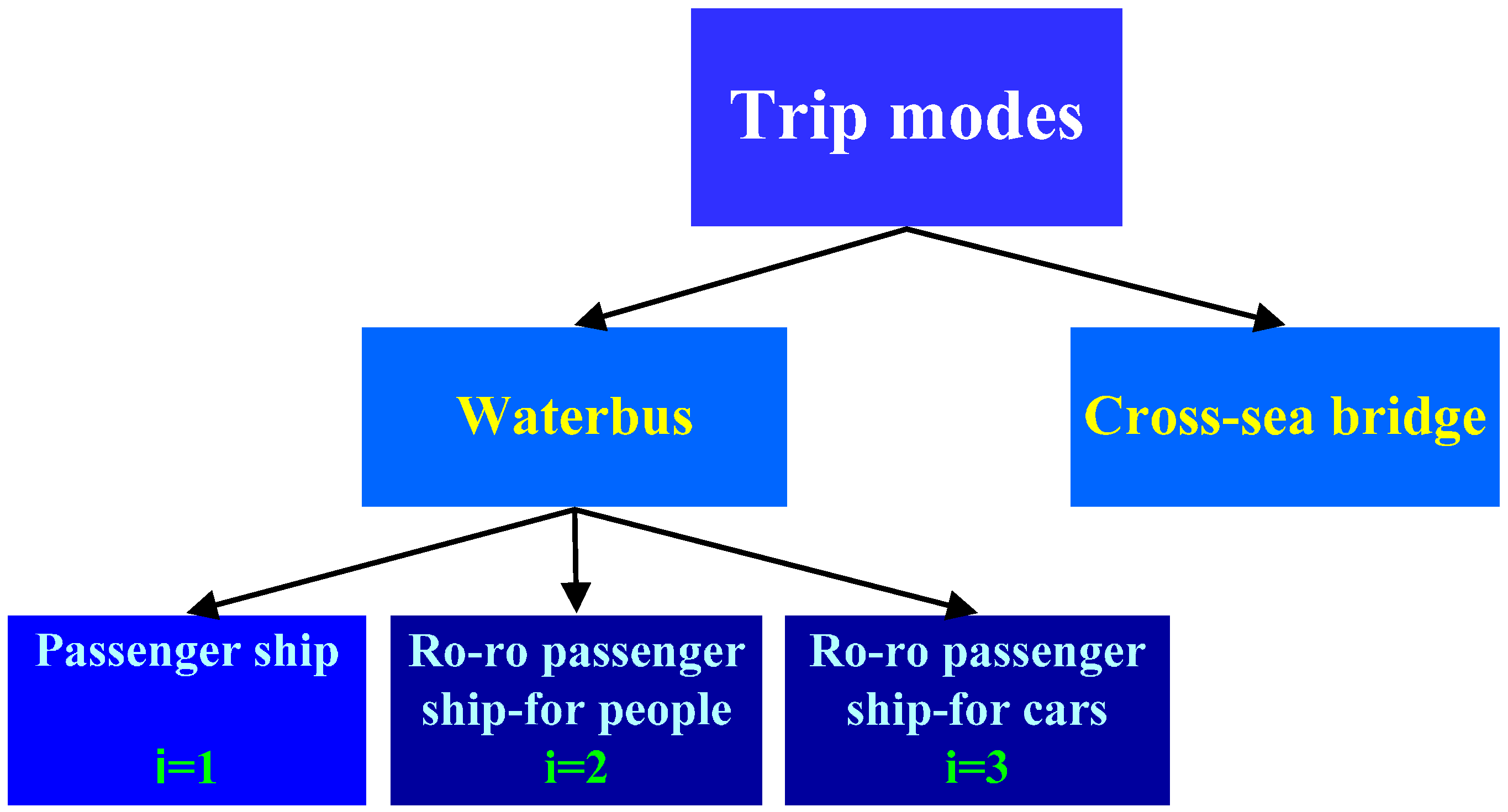
The trip time cost and the fares associated with each available mode are the attributes in this paper, which have impacts upon individuals’ transport behaviors. There are two travel modes for people to choose: waterbus and driving across cross-sea bridge. If people take the waterbus, there are three types of ships for them to choose from: the passenger ship, the ro-ro passenger ship for passengers, and the ro-ro passenger ship for cars. As alternatives are not independent, a Nested Logit model [29] is used to solve the traffic assignment problem. As is shown in Figure 3, the alternatives are the two mode choices (waterbus and drive across the cross-sea bridge). Additionally, there are two kinds of waterbuses (passenger ship and ro-ro passenger ship). Passenger ships can only carry passengers and ro-ro passenger ships can carry passengers as well as cars at the same time. For the convenience of calculation, the ro-ro passenger ship is divided into two kinds (for people and for cars) because it can both carry passengers and cars. The specific equations is as follows:

$$P_{ik}^w=\frac{e^{V_{ik}^w}}{{\displaystyle \sum _{i=1}^3{e}^{V_{\text{i}k}^w}}}\times \frac{e^{V_k^w}}{e^{\left(V_k^w+V_k^c\right)}}$$

(4)

$$P_k^w={\displaystyle \sum _{i=1}^3{P}_{ik}^w}$$

(5)

$$P_k^c=1-P_k^w$$

(6)

The utility is an equation of the attributes associated with that alternative, which is as follows:

$$V_{1k}^w=\text{α}\times c_{1k}^w+\text{β}\times C_{1k}^w+\text{γ}$$

(7)

$$V_{2k}^w=\text{α}\times c_{2k}^w+\text{β}\times C_{2k}^w+\text{θ}$$

(8)

$$V_{3k}^w=\text{α}\times c_{3k}^w+\text{β}\times C_{3k}^w$$

(9)

$$V_k^w=\ln \left(e^{V_{1k}^w}+e^{V_{2k}^w}+e^{V_{3k}^w}\right)$$

(10)

$$V_k^c={\text{α}}^{\text{'}}\times c_k^c+{\text{β}}^{\text{'}}\times C_k^c$$

(11)

where α, β, γ, θ, α′, β′ are unknown constants, among which α and α′ are the utility coefficients for traveling time costs and β and β′ are the utility coefficients for fares, respectively; γ and θ are the utility coefficients of comfort.

Constraint conditions are as follows:

$$q_{ik}^w\le E_i$$

(12)

$${\displaystyle \sum _k\left({\displaystyle \sum _{i=1}^{3}E{Q}_{ik}^w\times n_{ik}^w}+E{Q}_k^{car}\times \frac{q_k^{car}}{\text{μ}}\right)}\le {\displaystyle \sum _k\left(E{Q}_k^c\times \frac{q_k}{\mu }\right)}$$

(13)

Equation (12) ensures that the number of waterbus passengers must be no greater than the capacity limit. Equation (13) means that the carbon emissions after optimizing cannot be greater than before.

Figure 3. The structure of the Nested Logit model.

Figure 3. The structure of the Nested Logit model.

4. Solution Algorithm

The bi-level model is a NP (Non-deterministic Polynomial)-hard problem that is mostly solved by heuristic algorithm. In this paper, the upper-level model is a multiple objective model optimizing the waterbus operation plan. The lower-level model is a traffic model split, which can be solved by general software. In this paper, we use the Lingo program to solve the parameters of the lower-level model. The multiple objective model of the upper-level model is solved using a NSGA-II algorithm.

The NSGA-II (Non-dominated Sorting Genetic Algorithm-II) algorithm proposed by Deb et al. [29,34] is one of the most efficient and famous multiple objective algorithms. The fast non-dominated sorting technique and a crowding distance are used to rank and select the population fronts in the algorithm. After that, the algorithm uses the standard bimodal crossover and polynomial operators to combine the current population and its offspring generated as the next generation. Lastly, the best individuals in terms of non-dominance and diversity are selected as the solutions. The specific process of the NSGA-II algorithm is shown as the following:

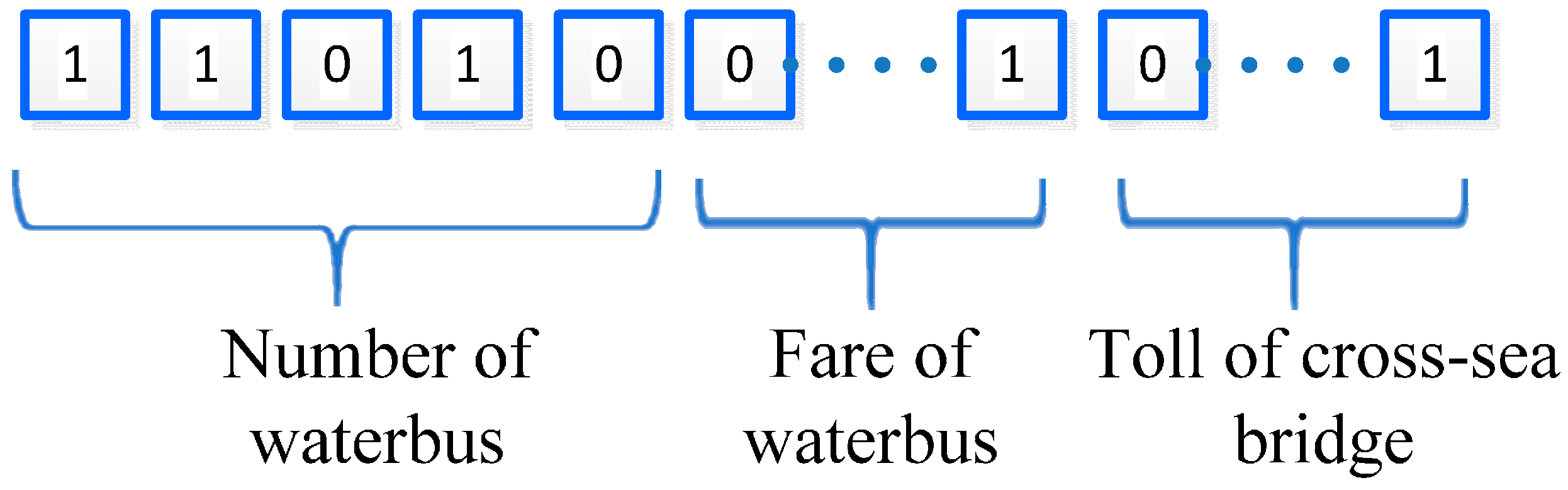
Step 1. Generating the initial population P_t. Let t = 0. The decision variables are the waterbus number, the fares, and the toll of the cross-sea bridge. Therefore, the coding of the algorithm consists of the waterbus number, the fares, and the toll of the cross-sea bridge. The coding is shown in Figure 4. The whole coding is encoded by binary. The first part of the coding represents the waterbus number, the second part represents the waterbus fares, and the third part represents the toll of the cross-sea bridge.

Figure 4. The meaning of NSGA-II algorithm coding.

Figure 4. The meaning of NSGA-II algorithm coding.

Step 2. Generate a new population Q_t by repeating the following steps: (1) choose two parent chromosomes from a population; (2) crossover operation (crossover is the operation that causes part of the structure of the two parent individuals to replace and restructure, and it also generates new individuals); (3) mutation operation (with a mutation there is a chance to mutate new offspring at each locus); (4) place the new offspring in the new population.

Step 3. Combine the parent population $P_t$ with the offspring population $Q_t$ and create a new alternative population, $R_t=P_t\cup Q_t$.

Step 4. Rank population $R_t$ by the following steps: (1) let rank counter $r=0$; (2) increase: $r=r+1$; (3) find the non-dominated individuals from the population $R_t$; (4) assign rank r to these individuals; (5) remove these individuals from population $R_t$; (6) if population $R_t$ is empty, stop. Otherwise, go to Step (2).

Step 5. Calculate the crowding distance by the following steps: (1) let $d_i=0$ for $i=1,2,\mathrm{...}Z$; (2) let $d_i$ and $d_z$ be maximum values, for example $d_i=d_Z=\infty$; (3) each objective equation is $f_k$, $k=1,2,\mathrm{...}m$; (4) for $j=2$ to $Z-1$, set $d_j=d_j+\left(f_{k_{j+1}}-f_{k_{j-1}}\right)$; (5) crowding selection operator x > y if $r_x=r_y$ and $d_x$ > $d_y$; (6) use new generated population for a further run of the algorithm; (7) if the established number of generations is reached, stop and return to the Pareto frontier [35] of the best solution in the current population. Otherwise, go to Step 2.

To explain the NSGA-II algorithm, a small numerical example is proposed in this paper. It is assumed that there are two objective equations:

$$\min f_1=x_1+x_2$$

(14)

$$\min f_2=x_1-x_2 x_1, x_2\in [1,5]$$

(15)

The values of $x_1$ and $x_2$ range from 1 to 5. When $x_1$ and $x_2$ get the minimal value at the same time, the objective equation 1 reaches the minimum. At the moment, the value of $x_1$ is 1 and the value of $x_2$ is also 1. When $x_1$ gets the minimal value and $x_2$ gets the maximal value, the objective equation 2 reaches the minimum. At this time, $x_1=1$ and $x_2=5$. The two objective equations cannot reach the minimum at the same time, so we use the NSGA-II algorithm to solve the problem. The solving process of the numerical example is as follows.

First, we generate the initial population $x_1=x_2=5$, $x_1=x_2=4$ and transfer the values into binary format: $x_1=x_2=101$, $x_1=x_2=100$. After that, carry on crossover and mutation and generate new offspring: $\begin{array}{cc}{x}_1=100& x_2=101\end{array}$, $\begin{array}{cc}{x}_1=010& x_2=011\end{array}$. Place new offspring in the new population: $x_1=x_2=101$, $x_1=x_2=100$, $\begin{array}{cc}{x}_1=100& x_2=101\end{array}$, $\begin{array}{cc}{x}_1=010& x_2=011\end{array}$. 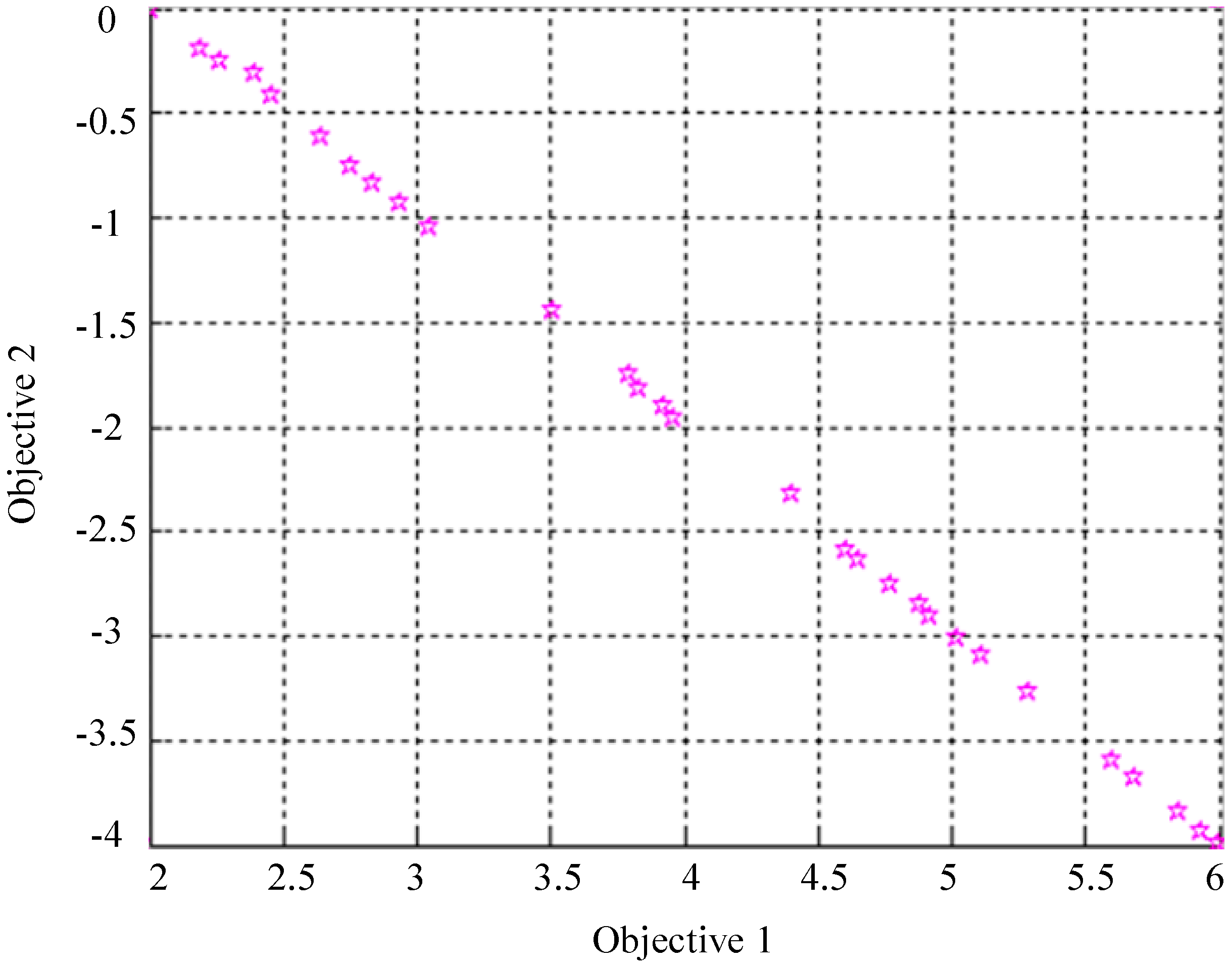Then, find the non-dominated individuals from the population: $x_1=x_2=100$, $\begin{array}{cc}{x}_1=010& x_2=011\end{array}$ and add them to the Pareto frontier. Finally, repeat the process and the maximum iteration number is set to 200 generations. The result of the small numerical example is shown in Figure 5. As shown in Figure 5, each point represents a set of decision variables and each point is an optimal solution.

Figure 5. Pareto frontier of the small numerical example.

Figure 5. Pareto frontier of the small numerical example.

5. Case Study

In order to test the above model and algorithm, the trip between Ningbo and Zhoushan Island has been chosen as a research example. As Figure 2 shows, this paper optimizes the waterbus operation plan of Line 1 and Line 2.

5.1. Related Parameters

5.1.1. Parameters of the Upper-Level Model

For Line 1 (from Baifeng of Ningbo to Yadanshan of Zhoushan Island) and Line 2 (from Baifeng of Ningbo to Shenjiamen of Zhoushan Island), the path length of the waterbus is 14.8 km and 27.4 km, respectively. The path length of the cross-sea bridge is 34.47 km. This paper assumes that the destination of the passengers is the center of Zhoushan Island for convenience of calculations. There is 9.1 km from Yadanshan to the center (Line 1) and 14.1 km from Shenjiamen to the center (Line 2). The distance from the cross-sea bridge to the center of Zhoushan Island is 13.5 km.

The vessel type and sailing speed are set in accordance with Zhoushan’s existing ships: the rated number of passengers is 200, and the speed of the ships is 15 km/h. The existing operational ships in Zhoushan are used as waterbuses to utilize existing resources, and only the depreciation costs of these ships are considered. The fuel cost is 7.5 RMB/liter, or $7500/ton. Other relevant data were shown in Table 2.

Table 2. The related parameters for solving the model.

	Waterbus			Cross-Sea Bridge
	Passenger Ship	Ro-ro Passenger Ship-for People	Ro-ro Passenger Ship-for Cars
Ship price	120	200	200	-
Fuel consumption	6.0 kg/km	8.0 kg/km	8.0 kg/km	0.1 L/km
Capacity	200	350	30	-
Emission factors	3.17	3.17	3.17	(${\text{η}}_1$, ${\text{η}}_2$, ${\text{η}}_3$, ${\text{η}}_4$) = (3952.113, −3.061, 0.029, 223.289)
Emission cost factor $\text{ε}$	4	4	4	4
Time cost factor $d^t$	2	2	2	2

Table 2. The related parameters for solving the model.

	Waterbus			Cross-Sea Bridge
	Passenger Ship	Ro-ro Passenger Ship-for People	Ro-ro Passenger Ship-for Cars
Ship price	120	200	200	-
Fuel consumption	6.0 kg/km	8.0 kg/km	8.0 kg/km	0.1 L/km
Capacity	200	350	30	-
Emission factors	3.17	3.17	3.17	(${\text{η}}_1$, ${\text{η}}_2$, ${\text{η}}_3$, ${\text{η}}_4$) = (3952.113, −3.061, 0.029, 223.289)
Emission cost factor $\text{ε}$	4	4	4	4
Time cost factor $d^t$	2	2	2	2

5.1.2. Parameters of the Lower-Level Model

In the Nested Logit model, the unknown parameters α, β, γ, θ, α′, β′ are determined by the individual point of view. By fitting and analyzing the existing data using the least squares method, the coefficient associated with each mode is calculated: $\text{α}=-0.079$, $\text{β}=-0.003$, ${\text{α}}^{\prime }=-0.065$, ${\text{β}}^{\prime }=-0.004$, $\text{γ}=0.39$, and $\text{θ}=0.47$. Both the values of the coefficients associated with fares and travel time costs are negative, which indicates that the utility associated with the alternative decreases with respect to rises in fares or travel time costs.

5.2. Calculation Results

Figure 6 shows the Pareto frontier for triple-objective optimization (the upper-level model) obtained using the NSGA-II algorithm. The population size of the NSGA-II algorithm is 100 and the crossover rate is set as 0.7, the mutation rate is 0.1, and the target M is 3, which means that the number of the objective equation is three, and the maximum iteration number is 3000 generations. Each point in Figure 6 represents a set of decision variables, which include the number and fare of waterbuses as well as the toll of cross-sea bridge. The three coordinate values of each point are the values of the three objective equations, which are the travel costs of people, the operation costs of operators, and carbon emission costs of the transportation system. The x-axis represents the value of objective Equation (1). The value of objective Equation (2) is on the y-axis, and the value of objective Equation (3) is on the z-axis. All the points of the Pareto frontier are optimal solutions which can minimize the travel costs of passengers, the waterbus operation costs of operators, and the carbon emissions of the system, respectively. In addition, the optimal solutions are widely distributed, which guarantees the diversity of the optimal solutions. Thus, the policymakers are provided with many solutions to choose from.

Figure 6. Pareto frontier for triple-objective optimization (the upper-level model).

Figure 6. Pareto frontier for triple-objective optimization (the upper-level model).

Considering the carbon emissions, the ideal solution to minimize the carbon emissions is selected. The results are shown in Table 3, Table 4 and Table 5.

Table 3. Waterbus operation plan of Line 1.

Line 1	Waterbus
	Passenger Ship	Ro-ro Passenger Ship-for People	Ro-ro Passenger Ship-for Cars
Number of ferry	15	8	8
Departure Frequency	8 min	20 min	20 min
Fares	15	15	70

Table 3. Waterbus operation plan of Line 1.

Line 1	Waterbus
	Passenger Ship	Ro-ro Passenger Ship-for People	Ro-ro Passenger Ship-for Cars
Number of ferry	15	8	8
Departure Frequency	8 min	20 min	20 min
Fares	15	15	70

Table 4. Waterbus operation plan of Line 2 during the non-workday.

Line 2	Waterbus
	Passenger Ship	Ro-ro Passenger Ship-for People	Ro-ro Passenger Ship-for Cars
Number of ferry	18	10	10
Departure Frequency	12 min	30 min	30 min
Fares	16	16	80

Table 4. Waterbus operation plan of Line 2 during the non-workday.

Line 2	Waterbus
	Passenger Ship	Ro-ro Passenger Ship-for People	Ro-ro Passenger Ship-for Cars
Number of ferry	18	10	10
Departure Frequency	12 min	30 min	30 min
Fares	16	16	80

Table 5. Waterbus operation plan of Line 2 during the workday.

Line 2	Waterbus
	Passenger Ship	Ro-ro Passenger Ship-for People	Ro-ro Passenger Ship-for Cars
Number of ferry	10	4	4
Departure Frequency	28 min	96 min	96 min
Fares	16	16	80

Table 5. Waterbus operation plan of Line 2 during the workday.

Line 2	Waterbus
	Passenger Ship	Ro-ro Passenger Ship-for People	Ro-ro Passenger Ship-for Cars
Number of ferry	10	4	4
Departure Frequency	28 min	96 min	96 min
Fares	16	16	80

As was shown in Table 3, the best operation plan of Line 1 is 23 waterbuses, which includes 15 passenger ships and eight ro-ro passenger ships. The departure frequency and fares of the passenger ship are 8 min and 15 RMB for each person, respectively. The departure frequency of the ro-ro passenger ship is 20 min and the fare is 15 RMB for each person or 70 RMB for each car.

Table 4 shows the waterbus operation plan of Line 2 during the non-workday. The best operation plan of Line 2 during the non-workday is 28 waterbuses, including 18 passenger ships and 10 ro-ro passenger ships, and the departure frequency of the two kinds of waterbus is 12 min and 30 min, respectively. In addition, the fare of the passenger ship is 16 RMB for each person and the fare of ro-ro passenger ship is 16 RMB for each person or 80 RMB for each car.

The waterbus operation plan of Line 2 during the workday is shown in Table 5. The best operation plan of Line 2 during workday is 14 waterbuses, which includes 10 passenger ships and four ro-ro passenger ships. The departure frequency of the two kinds of waterbus is 28 min and 96 min, respectively. The fare of the passenger ship is 16 RMB for each person and the fare of the ro-ro passenger ship is 16 RMB for each person or 80 RMB for each car, which is the same as on the workday. After optimizing, the toll of the cross-sea bridge increases to 140 RMB for each car from the original 120 RMB for each car.

Figure 7 compares the traffic of each mode after optimizing and the traffic of each mode before optimizing. It can be seen in Figure 7 that the traffic of the cross-sea bridge decreases 32.7% after optimizing. It decreases to 15,468 people, which is equivalent to 10,312 cars. Additionally, the saturation of the cross-sea bridge is about 0.5 at that moment. Though the saturation after optimizing is still higher than the average of the expressway, it is observably lower than before. The traffic congestion of the cross-sea bridge is alleviated after optimizing. The traffic of the waterbus increases both on Line 1 and Line 2. The growth of the traffic on Line 1 is bigger than on Line 2, whether during the non-workday or the workday. The reason for this is that Line 1 is closer to the center of Zhoushan Island than Line 2 and the traffic of the cross-sea bridge is more likely to transfer to Line 1 as compared to Line 2. In addition, because Line 2 connects with the Putuo scenic zone, some travelers may choose to take the waterbus instead of driving across the cross-sea bridge after optimizing. Thus, the traffic of Line 2 during the non-workday obviously increases.

The Figure 8 compares the traffic of each mode after optimizing and the traffic of each mode before optimizing. After optimizing the waterbus operation plan, the carbon emission cost of the system decreases from 464,265.4 to 346,969. There is about a 25.3% decrease in the carbon emission cost and a 30.6% decrease in the travel cost of people. The reason for the decrease in the travel cost is that the fares of the waterbus are lower than the cross-sea bridge, and the more people that transfer to take waterbus, the less travel costs are paid from the system. At the same time, the operation cost of the operators increases 26.8% due to the increase of the waterbuses.

Figure 7. Contrast of traffic after optimizing with before optimizing.

Figure 7. Contrast of traffic after optimizing with before optimizing.

Figure 8. Contrast of costs after optimizing with before optimizing.

Figure 8. Contrast of costs after optimizing with before optimizing.

6. Conclusions

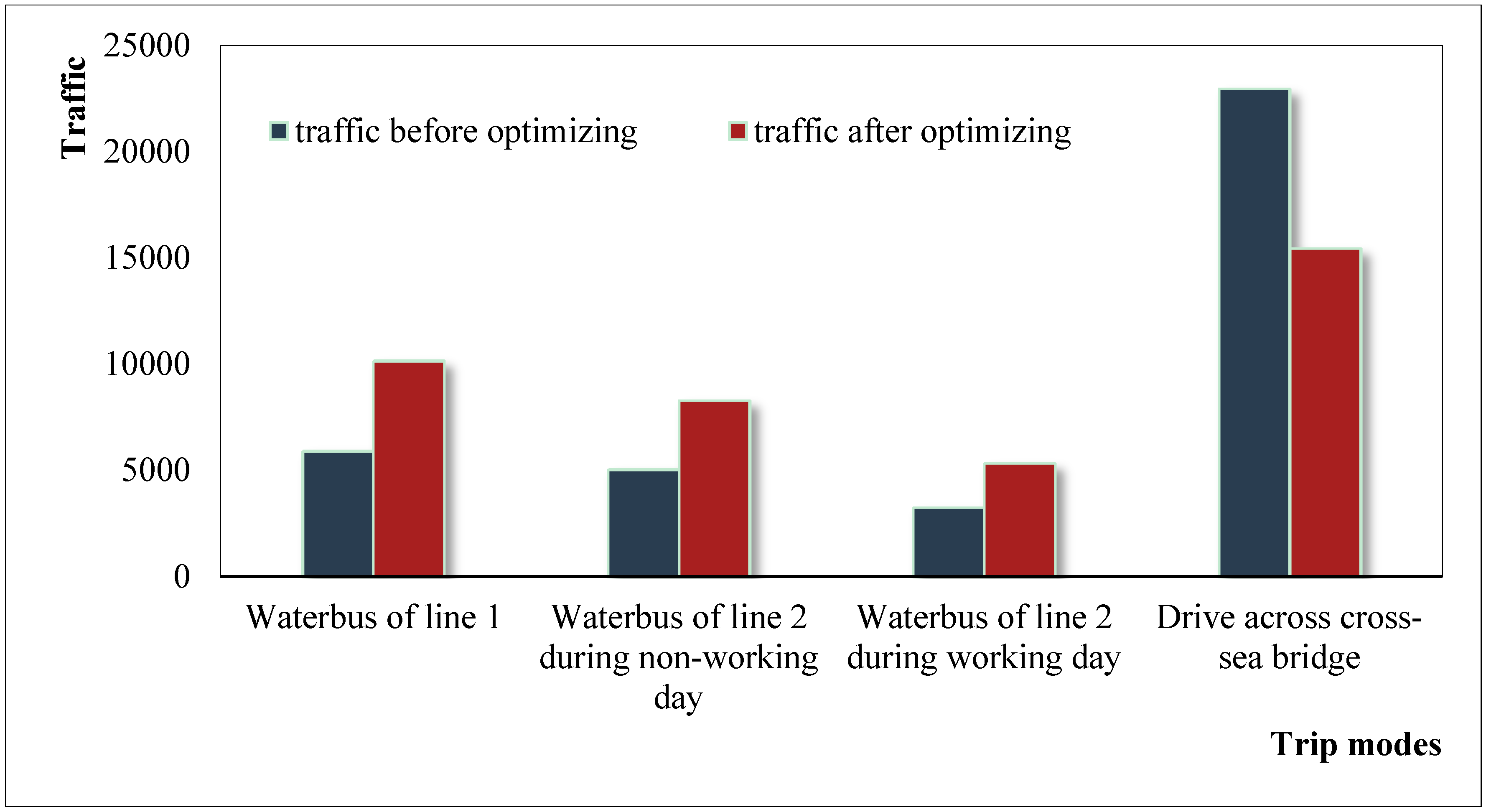
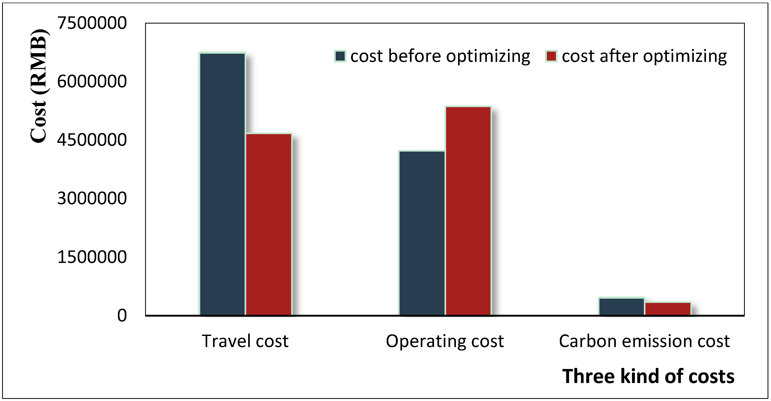
In order to cut the carbon emissions of the transport sector, this paper proposes a bi-level model that considers carbon emissions to optimize the waterbus operation plan. Meanwhile, the interests of both the passengers and the operators are also considered. The waterbus operation plan consists of departure frequency, fares, and the number of waterbuses on each line. Additionally, two kinds of ships are considered in this paper: passenger ships and ro-ro passenger ships. Moreover, the NSGA-II algorithm is used to solve the model. Finally, through the case study of Zhoushan Island, the results show that the proposed model in this paper can optimize the waterbus operation plan with the consideration of carbon emissions. After optimizing, 32.7% of overland traffic is transferred to the waterbus, which can alleviate the cross-sea bridge pressure and reduce the carbon emissions of the transport sector at the same time. In addition, the travel costs of passengers are lower than before, thus the plan is more likely to be accepted by the public. Though the operating costs increase after optimizing, toll revenue from the cross-sea bridge is used to subsidize the waterbus, and the income of the companies also increases as the traffic of the waterbus increases. Thus, the result of optimizing involves no harm for operators. Considering the interests of passengers, operators, and the environment, the plan we propose in this paper is feasible. Nevertheless, funds are one of the biggest hurdles in this plan. In regard to environmental protection and sustainable development, the government can take some measures to improve the feasibility of the waterbus operation plan; for example, the government can increase the subsidy of the waterbus and make some preferential policies for waterbus operators. This paper has significant practical meaning for Zhoushan Island.

References

1. Brazil, W.; Caulfield, B. Does green make a difference: The potential role of smartphone technology in transport behaviour. Transp. Res. Part C 2013, 37, 93–101. [Google Scholar] [CrossRef]
2. Pachauri, R.K.; Reisinger, A. (Eds.) Intergovernmental panel on climate change. In Climate Change 2007: Synthesis Report; IPCC: Geneva, Switzerland, 2007; p. 104.
3. Meinshausen, M.; Smith, S.J.; Calvin, K.; Daniel, J.S.; Kainuma, M.L.T.; Lamarque, J.F.; Matsumoto, K.; Montzka, S.A.; Raper, S.C.B.; Riahi, K.; et al. The RCP greenhouse gas concentrations and their extensions from 1765 to 2300. Clim. Chang. 2011, 109, 213–241. [Google Scholar] [CrossRef]
4. Barth, M.; Boriboonsomsin, K. Real-world carbon dioxide impacts of traffic congestion. Transp. Res. Rec.: J. Trans. Res. Board 2008, 2058, 163–171. [Google Scholar] [CrossRef]
5. Jiang, D.G.; Wu, Y.Z. A Planning Method of Urban Non-Motorized Traffic System—A Case from Hangzhou. Appl. Mech. Mater. 2012, 174, 2395–2398. [Google Scholar] [CrossRef]
6. Ye, L.; Yang, D.; He, N. Application of Stated Preference Survey Method in Waterbus System Design. Int. Conf. Trans. Eng. 2007, 40, 2453–2458. [Google Scholar]
7. Sato, K.; Takadama, K. Pittsburgh-style learning classifier system for multiple environments: Towards robust waterbus route for several situations. Int. J. Bio-Inspired Comput. 2011, 3, 370–383. [Google Scholar] [CrossRef]
8. Li, J.; Huang, S. Characteristics Analysis of Guangzhou Waterbus Passengers Based on IC Card Data. CICTP 2014. [Google Scholar] [CrossRef]
9. Keiji, S.; Keiki, T. Waterbus Route Optimization by Pittsburgh-style Learning Classifier System. In Proceedings of the SICE 2007 Annual Conference, Takamatsu, Japan, 17–20 September 2007; pp. 1150–1154.
10. Keiki, T.; Takahiro, M.; Daisuke, W.; Mitsujiro, K. Exploring Quantitative Evaluation Criteria for Service and Potentials of New Service in Transportation: Analyzing Transport Networks of Railway, Subway and Waterbus. In Intelligent Data Engineering and Automated Learning-IDEAL 2007; Springer: Berlin, German, 2007; Volume 4881, pp. 1122–1130. [Google Scholar]
11. Ortúzar, J.D.D.; Willumsen, L.G. Simplified Transport Demand Models, in Modelling Transport, 4th ed.; John Wiley & Sons, Ltd.: Chichester, UK, 2011. [Google Scholar]
12. Cascetta, E. Transportation Systems Analysis: Models and Applications, 2nd ed.; Springer: Pergamon, Turkey, 2009. [Google Scholar]
13. Lam, W.H.K.; Bell, M.G.H. Advanced Modeling for Transit Operations and Service Planning Hardcover; Emerald Group Publishing Limited: Pergamon, Turkey, 2002. [Google Scholar]
14. Russo, F.; Comi, V.A. Estimation of target time distribution for agri-food products by road transpor. In Schedule-Based Modeling of Transportation Networks: Theory and Applications; Wilson, N.H.M., Nuzzolo, A., Eds.; Springer Science and Business Media: New York, NY, USA, 2009; pp. 267–283. [Google Scholar]
15. Vitetta, A.; Cartisano, A.; Comi, A. Application for comparing frequency and schedule-based approaches in the simulation of a low frequency transit system. In Schedule-Based Dynamic Transit Modeling: Theory and Applications; Wilson, N.H.M., Nuzzolo, A., Eds.; Kluwer Academic Publishers: Boston, MA, USA, 2004; Volume 28, pp. 217–239. [Google Scholar]
16. Bloom, J.J.; Mathew, T.V. Intelligent Agent Optimization of Urban Bus Transit System Design. J. Comput. Civil Eng. 2011, 25, 357–369. [Google Scholar] [CrossRef]
17. Dubois, D.; Bel, G.; Libre, M. A set of methods in transportation network synthesis and analysis. J. Oper. Res. Soc. 1979, 30, 797–808. [Google Scholar] [CrossRef]
18. Baaj, M.H.; Mahmassani, H.S. Hybrid route generation heuristic algorithm for the design of transit networks. Transp. Res. Part C 1995, 3, 31–50. [Google Scholar] [CrossRef]
19. Agrawal, J.; Mathew, T.V. Transit route network sfesign using parallel genetic algorithm. J. Comput. Civil Eng. 2004, 18, 248–256. [Google Scholar] [CrossRef]
20. Yu, B.; Lam, W.H.K.; Tam, M.L. Bus arrival time prediction at bus stop with multiple routes. Transp. Res. Part C: Emerg. Technol. 2011, 19, 1157–1170. [Google Scholar] [CrossRef]
21. Shih, M.C.; Mahmassani, H.S. Vehicle sizing model for bus transit networks. Transp. Res. 1995, 1452, 35–41. [Google Scholar]
22. Chakroborty, P.; Deb, K.; Sharma, R.K. Optimal fleet size distribution and scheduling of transit systems using genetic algorithms. Transp. Plan. Technol. 2001, 24, 209–225. [Google Scholar] [CrossRef]
23. Cordeau, J.F.; Toth, P.; Vigo, D. A survey of optimization models for train routing and scheduling. Transp. Sci. 1998, 32, 380–404. [Google Scholar] [CrossRef]
24. Chakroborty, P. Genetic algorithms for optimal urban transit network design. Comput.-Aided Civil Infrastruct. Eng. 2003, 18, 184–200. [Google Scholar] [CrossRef]
25. Yao, B.Z.; Hu, P.; Lu, X.H.; Gao, J.J.; Zhang, M.H. Transit network design based on travel time reliability. Transp. Res. Part C 2014, 43, 233–248. [Google Scholar] [CrossRef]
26. Yu, B.Z.; Gao, J.J.; Zhang, M.H. An improved particle swarm optimization for carton heterogeneous vehicle routing problem with a collection depot. Ann. Oper. Res. 2014. [Google Scholar] [CrossRef]
27. Yu, B.; Yang, Z.Z. A Dynamic Holding Strategy in Public Transit Systems with Real-time Information. Appl. Intell. 2007, 31, 69–80. [Google Scholar] [CrossRef]
28. Coello, C.A.C. A comprehensive survey of evolutionary-based multiobjective optimization techniques. Knowl. Inform. Syst. 1999, 1, 269–308. [Google Scholar] [CrossRef]
29. Wen, C.H.; Koppelman, F.S. The generalized nested logit model. Transp. Res. Part B 2001, 35, 627–641. [Google Scholar] [CrossRef]
30. Yu, B.; Peng, Z.X.; Kong, L.; Cui, Y.; Wang, K.M. Optimization method for line planning and operation strategy of waterbus: the case of Zhoushan city. Oper. Res. 2015, 15, 25–49. [Google Scholar]
31. Zhu, S.L. Comparison of Transportation Energy Consumption and Greenhouse Gas Emission between Beijing and Shanghai. Urban Transp. Chin. 2010, 8, 58–63. [Google Scholar]
32. Yao, B.Z.; Hu, P.; Zhang, M.H.; Jin, M.Q. A Support Vector Machine with the Tabu Search Algorithm for Freeway Incident Detection. Int. J. Appl. Math. Computer Sci. 2014, 24, 397–404. [Google Scholar] [CrossRef]
33. Sun, H.; Si, B.F.; Wu, J.J. Combined Model for Flow Assignment and Mode Spilt in Two-modes Traffic Network. J. Transp. Syst. Eng. Inform. Technol. 2008, 8, 77–82. [Google Scholar]
34. Deb, K.; Agrawal, S.; Pratap, A.; Meyarivan, T. A fast elitist non-dominated sorting genetic algorithm for multi-objective optimization: NSGA-II. In Lecture Notes in Computer Science; Springer: Berlin, German, 2000; Volume 1917, pp. 849–858. [Google Scholar]
35. Salazar, F.J.T.; Macau, E.E.N.; Winter, O.C. Pareto Frontier for the time-energy cost vector to an Earth-Moon transfer orbit using the patched-conic approximation. Comput. Appl. Math. 2015, 34, 461–475. [Google Scholar] [CrossRef]