Investment Strategy of Emission-Reduction Technology in a Supply Chain

Abstract

Greenhouse gas emissions have serious impacts on the natural environment. Therefore, the restrictions imposed on carbon emission force enterprises to take carbon emission into consideration when making production decisions. In this paper, in the context of allowing emission trading and investment of emission reduction technology, models were presented for a two-stage supply chain to analyze the optimal investment and pricing decisions. The results indicate that manufacturer’s endurance capacity of reduction difficulty is higher in the cooperation model than in the Stackelberg game model, and that perfect coordination of supply chains can be realized by a revenue sharing contract. From the perspective of a consumer, low-carbon products mean higher price, so that subsidies or tax exemptions should be provided to keep low prices. Meanwhile, the government can promote investment in emission-reduction technologies and achieve its emission reduction targets by controlling emission trading price, strengthening emission reduction publicity and providing technology investment subsidies.

1. Introduction

The rapid growth of the world economy and continuous adjustment of economic structures are leading to a substantial increase in energy demand. At the same time, environmental issues and consequences caused by energy use have been gradually recognized, of which carbon emission is one of the biggest concerns. The Intergovernmental Panel on Climate Change (IPCC) fourth assessment report, released in November 2007, concluded: Climate warming was mainly attributed to the large amount of greenhouse gases emitted by human industrial activities like carbon dioxide and methane, of which the greenhouse effect caused by carbon dioxide accounted for 50% [1].

Since climate security has become a public interest, the Kyoto Protocol, entering into force on February 16, 2005, set emission limits at the national level for developed countries for the first time so as to mitigate global warming and avoid catastrophic effects on humans. This protocol put forward three flexible mechanisms to reduce emissions and is legally binding for all contracting parties.

International emission trading, the most remarkable of the three flexible reduction mechanisms, is a market-based approach to reduce emissions by combination of direct control and economic incentives. A central authority (usually a governmental body) first sets a limit or cap on the amount of emissions that can be emitted, and then the limit or cap is allocated to economic entities in the form of emissions permits, which represents the right to emit or discharge a specific volume of the specified pollutant. Trading of emission permits is allowed so as to achieve total control of emissions, and emission-dependent firms should self-regulate based on emission limits; namely, firms requiring the use of excessive emissions must purchase additional emission permits from other organizations through the emissions-trading market (or face legal action), while those requiring fewer permits (emission savings obtained through carbon reduction measures) can get additional revenue through selling emission permits.

China is the world’s largest emitter of carbon dioxide. The Chinese State Council has issued the twelfth national five-year plan work program to control greenhouse gas emissions in January 2012, which proposed an emission reduction target of 17% less national carbon dioxide emissions per unit of GDP in 2015 compared to 2010. At present, Beijing, Tianjin, Shanghai, Chongqing, Guangdong, Hubei, and Shenzhen have been chosen as the pilot cities with emission trading. On this basis, China will gradually promote the construction of a domestic carbon trading market. It is foreseeable that carbon emission trading mechanisms will play an important role in the future of emission-reduction practices.

Cooperation in a supply chain enables the participators to create and capture mutual benefits including profit enhancements, cost reductions, and operational flexibility to cope with high demand uncertainties. Recently, considering various requirements from customers, government and corporate social responsibility, firms that design and operate supply chains are particularly sensitive to the reduction of their carbon emission. Therefore, it is very necessary to study emission-reduction cooperation strategies with the consideration of emission trading policies on the level of supply chain.

The article analyses the consequences of emission-trading regulatory policy on supply chain decisions—pricing and investment in carbon reduction technology. To clarify, we do not consider a capacity investment problem in this paper. What we considered is that the supply chain member (the manufacturer) can make an investment in improving production technology’s cleanliness. The objective of this paper is to contribute to the strategies of coordinating emission-reduction effort across supply chains. The rest of this paper is organized as follows. Section 2 reviews the relevant literature. Section 3 describes the research topics and introduces the relevant assumptions and notions. Section 4 presents the model and analyzes the profit of supply chain members in three scenarios. Then, comparisons of the three models are presented in Section 5. Further, Section 6 gives a numerical example and provides a sensitivity analysis to show the application of our models, together with several valuable managerial insights as well. Finally, concluding remarks and future research ideas are given in Section 7.

2. Literature Review

Currently, research in emission trading mostly focuses on the macro level, such as the effects of emission reduction policies on national economy. Ghosh et al. [2] studied the impacts of carbon emission on the Indian economy, and showed that any effort to reduce carbon emissions would lead to a decline in national income in the short term. Taking carbon dioxide and sulfur dioxide as environmental indicators and GDP as an economic indicator. Fodha et al. [3] investigated the correlation between economic development and emissions in Tunisia, and their research confirmed the long-term coordination between per capita emissions and per capita GDP; namely, emission reduction policies and investments would not damage economic growth.

Similarly, for energy-intensive industries such as steel industry, electric power industry, and petrochemical industry, commercialization of emission permits is bound to change their profit model and cost structure, thereby affecting their production behaviors. As a consequence, relevant research in energy-intensive industries has been widely carried out to provide useful advises for their development [4,5,6,7].

The restrictions imposed on carbon emission and the establishments of cap-and-trade schemes force enterprises to take carbon emission into consideration while making production operation decisions. Nowadays, harmonization between enterprise self-interest and environment protection has become an extensive consensus for all parties. Although there are vast studies on the supply chain related to low-carbon [8] (Lam et al., 2009), research on emission reduction policies that impact enterprise and supply chain operations at the micro level is still limited.

Benjaafar et al. [9] conducted groundbreaking research on carbon emission operation issues by incorporating carbon emission factors into an enterprise’s decision-making model, which produced numerous significant management implications. Associating carbon footprint parameters with various decision variables, they modified traditional models to support decision-making that accounted for both cost and carbon footprint, and examined how the values of these parameters, as well as the parameters of regulatory emission control policies, affected cost and emissions. Hua et al. [10] investigated how firms managed carbon footprints in inventory management under the carbon emission trading mechanism. Aiming at maximizing the profits of the whole supply chain system, Zhao et al. [11] constructed a low-carbon supply chain model and discussed how marginal abatement cost efficiency and emission trading price influenced optimal emission reductions. Du et al. [12] considered the government-allocated emission cap of an emission-dependent manufacturer as a kind of environmental policy and formally investigated its influence on decision-making within the concerned emission-dependent supply chain, as well as distribution fairness in social welfare. Caro et al. [13] introduced a model of joint production of GHG emissions in general supply chains, decomposed the total footprint into each process of which can be influenced by any combination of firms. They analyzed two main scenarios. In the first scenario, the social planner allocates emissions to individual firms and imposes a cost on them in proportion to the emissions allocated. In the second scenario, a carbon leader voluntarily agrees to offset all emissions in the entire supply chain and then contracts with individual firms to share the costs of those offsets. They found that, in order to induce the optimal effort levels, the emissions need to be double counted. This is in contrast to the usual focus in the life-cycle assessment and carbon footprinting literatures on avoiding double counting. Song et al. [14] investigated the single-period problem under three carbon emissions policies and obtained the optimal production quantity accordingly. Considering carbon emissions of transport, Rosič et al. [15] evaluated the economic and environmental sustainability of dual sourcing under two different regulations and found that emission trading was superior to an emission tax on transportation from the perspective of policy-making and management. Konur and Schaefer [16] analyzed the integrated inventory control (with the basic EOQ model) and transportation decisions (LTL and TL carriers) of a retailer under four different carbon emission regulation policies. It was observed that both transportation costs and transportation emissions of the carriers may affect the retailer’s preference. Toptal et al. [17] analyzed a retailer’s joint decisions on inventory replenishment and carbon emission reduction investment under three carbon emission regulation policies, and extended their research through considering the existence of environmentally sensitive customers. Choi [18] studied how to design carbon footprint taxation scheme to apply to a QR system to enhance environmental sustainability. He et al. [19] proposed two representative modes for carbon emission reduction-vertical transfer payment contract and third-party carbon emission reduction service providers. They analyzed the corresponding Stackelberg game for each model and compared emission reduction effectiveness. Wang et al. [20] consider a problem of choosing an appropriate channel for the marketing channel structure of remanufactured fashion products. Han et al. [21] incorporate both price competition and service competition into a supply chain model of a manufacturer and two competing retailers.

Based on emission-reduction policies, all studies mentioned above take emission factors into account when analyzing optimal production operation decisions. Our study shares a similar motivation, but has a more specific focus. Given the necessity of emission-reduction technology investment in low-carbon economy, instead of adding different kinds of costs such as inventory cost, transportation cost, etc., we add an emission-reduction technology input cost (dependent on the emission reduction level), which can produce positive income through sales revenue and emission cost savings. Then, we study the corresponding effect on optimal investment and pricing decisions of collaboration among firms within the same supply chain that undertake emission-reduction technology investment and allow emission trading. Furthermore, we investigated the impact of various exogenous parameters on the emission reduction investment, as well as the performance of emission reduction.

Ghosh and Shah [22] focus on a very similar setting to this paper. By using game theoretic models, they show how greening levels, prices and profits are affected by supply chain decision structure and propose a two-part tariff contract to coordinate the green channel. The key difference between their work and ours is that we consider the cap-and-trade regulatory policy in our model which is not taken into account in Ghosh and Shah [22]. We investigate the impact of cap-and-trade regulatory policy on the supply chain’s pricing decision as well as investment decision. Another difference is that we use revenue sharing contract to coordinate the channel while a two-part tariff contract is used to coordinate the channel in Ghosh and Shah’s model [22].

3. Model Description

Consider a supply chain consists of a single manufacturer and a single retailer. With the present technology, the manufacturer produces each unit of product at marginal cost c and as a byproduct of the production process, e₀ units of emissions is released with per unit of output. The manufacturer is subject to a cap-and-trade regulation, C_g is the emission quota allocated by the government and r is the buying/selling price for per unit emission permit. The manufacturer can make an investment in his production technology to make it cleaner. With investment I(α), the manufacturer can reduce the per unit emissions by α percentage while not change the unit production cost. We assume the investment cost function, I(α), is continuously differentiable with $I\text{'}(\alpha )>0,I^{″}(\alpha )>0$ and $I(0)=0,I(1)\to \infty$. To be specific, we further assume the investment cost function, I(α) is given as

$$I(\alpha )=-k\ln (1-\alpha ),\alpha \in (0,1)$$

(1)

where k is a coefficient which measures emission reduction difficulty for the manufacturer. It is easy to verify that $I\text{'}(\alpha )>0,I^{″}(\alpha )>0$ and $I(0)=0,I(1)\to \infty$ are satisfied. The manufacturer sells her products to the retailer and then the retailer sells to the market. Following Ghosh et al. (2012), the market demand is assumed to be linear and given by

$$D(p,\text{α})=a-p+\text{λα}$$

(2)

where p (<a) is the retail price and a is market size. λ is a coefficient that measures the impact of emission reduction on market demand, and we name it consumer preference coefficient of low carbon. With a high λ, the demand is more sensitive to α.

The following assumptions are also needed in our model:

A1. 

All players (the manufacturer, the retailer) are rational and pursue profit maximization.

A2. 

The manufacturer and retailer are under symmetric information in consumers’ preference of low carbon.

A3. 

There is no transaction cost in the emission trade market and the market is well-supplied.

A4. 

The carbon price is independent of the manufacturer’s decisions.

The notation is presented below:

a	The market potential
Cg	The emission quota allocated by the government
c	Production cost per unit product
w	Decision variable, wholesale price per unit product
p	Decision variable, selling price per unit product
p	Decision variable, selling price per unit product
r	Selling/Buying price per unit emission permit
e0	Carbon emissions per unit product
k	Difficulty coefficient of emission reduction
λ	Consumer preference coefficient of carbon
α	Decision variable, the percentage of emission reduction per unit product
I(α)	Investment cost function,
D(p,α)	Market demand function

4. Models with Emission-Reduction Investment

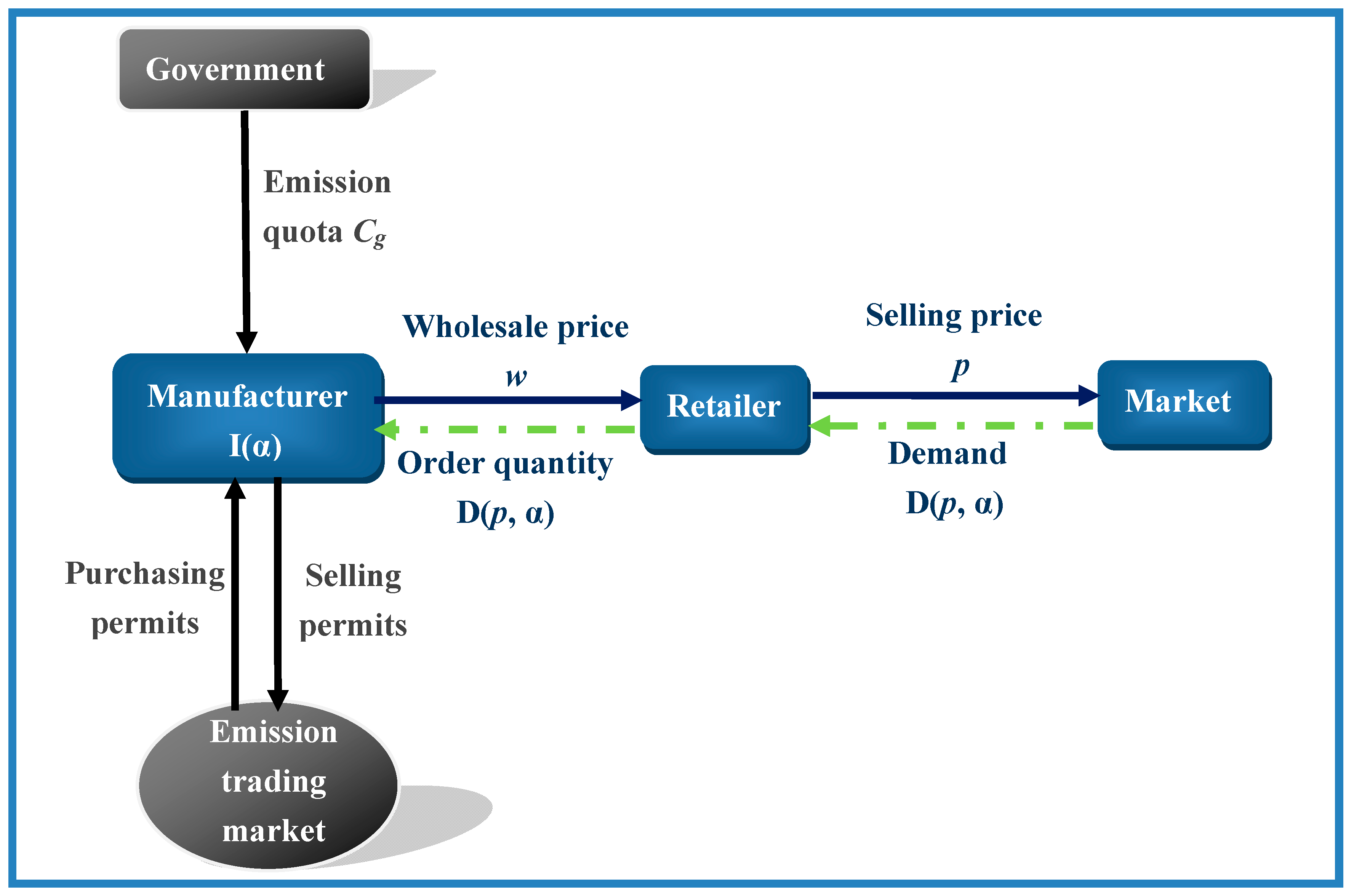
In this section, we present three models, Stackelberg Model (SM), Cooperation Model (CPM) and Coordination Model (CM). In the Stackelberg Model, the manufacturer is the leader since she determine the emission reduction level and wholesale price first, then she sells her products to the retailer with a simple wholesale price contract (See Figure 1). In the Cooperative Model, the manufacturer and the retailer is cooperated as a single firm. In the Coordination Model, the manufacturer uses a revenue sharing contract to trade with the retailer.

Figure 1. Stackelberg Model.

Figure 1. Stackelberg Model.

4.1. Stackelberg Model

In the Stackelberg Model, the manufacturer first determines the wholesale price w and the emission reduction investment I(α), or equivalently the unit emission reduction percentage α. Knowing α and w, the retailer chooses the retail price p to maximize his own profit. We analyze the two-stage Stackelberg game from backwards to derive the Stackelberg-Nash equilibrium.

In the second stage, the retailer’s problem can be formulated as follows:

$$\underset{p}{\max }{\text{π}}_R^{SM}(p)=(p-w)(a-p+\text{λα})$$

(3)

Given w and α, the optimal retail price for the retailer is

$$p^{SM}(w,\text{α})=\frac{a+\text{λα}+w}{2}$$

(4)

Anticipating the retailer’s best response, in the first stage the manufacturer determines the wholesale price w and the unit emission reduction percentage α to

$$\underset{w,\text{α}}{\max } {\text{π}}_M^{SM}(w,\text{α})=(w-c)(a-p^{SM}(w,\text{α})+\text{λα})-r\left[e_0(1-\text{α})(a-p^{SM}(w,\alpha )+\lambda \alpha )-C_g\right]+k\ln (1-\alpha )$$

(5)

In the Stackelberg-Nash equilibrium, the wholesale price, the emission reduction percentage, the retail price and the corresponding profits of manufacturer and retailer are given below (proof see Appendix 1):

$$w^{SM*}=\frac{1}{2}(a+c+r{e}_0)+\frac{1}{4}(\lambda -r{e}_0)\frac{(\lambda +2r{e}_0-a+c)+\sqrt{{(\lambda +a-c)}^2-16k}}{\lambda +r{e}_0}$$

(6)

$${\alpha }^{SM*}=\frac{(\lambda +2r{e}_0-a+c)+\sqrt{{(\lambda +a-c)}^2-16k}}{2(\lambda +r{e}_0)}$$

(7)

$$p^{SM*}=\frac{1}{4}(3a+c+r{e}_0)+\frac{1}{8}(3\lambda -r{e}_0)\frac{(\lambda +2r{e}_0-a+c)+\sqrt{{(\lambda +a-c)}^2-16k}}{\lambda +r{e}_0}$$

(8)

$${\pi }_R^{SM*}=\frac{1}{64}{\left[a-c+\lambda +\sqrt{{(\lambda +a-c)}^2-16k}\right]}^2$$

(9)

$${\pi }_M^{SM*}=\frac{1}{32}{\left[a-c+\lambda +\sqrt{{(\lambda +a-c)}^2-16k}\right]}^2+k\ln (1-\frac{(\lambda +2r{e}_0-a+c)+\sqrt{{(\lambda +a-c)}^2-16k}}{2(\lambda +r{e}_0)})+r{C}_g$$

(10)

Note that to ensure the above values be real number, the emission reduction difficulty coefficient, k should satisfy:

$$k\le {(\frac{\lambda +a-c}{4})}^2$$

(11)

Proposition 1.

(i)

$\frac{\partial {\alpha }^{SM*}}{\partial k}<0$.

(ii)

$\frac{\partial {\alpha }^{SM*}}{\partial r}>0,\frac{\partial {\alpha }^{SM*}}{\partial {\text{C}}_g}=0$.

(iii)

if $k<\frac{1}{4}{\xi }_2(2{\xi }_1+{\xi }_2)$, $\frac{\partial {\alpha }^{SM*}}{\partial \lambda }>0$.

where ${\xi }_{\text{1}}=\frac{\text{1}}{\text{2}}（\lambda \text{+}r{e}_0），{\xi }_{\text{2}}=\frac{\text{1}}{\text{2}}\text{(a}-\text{c}-r{e}_0\text{)}$.

Proof. From Equation (7), we have

$$\begin{array}{l}\frac{\partial {\alpha }^{SM*}}{\partial k}=-\frac{4}{(\lambda +r{e}_0)\sqrt{{(\lambda +a-c)}^2-16k}}<0\\ \frac{\partial {\alpha }^{SM*}}{\partial r}=\frac{e_0[(\lambda +a-c)-\sqrt{{(\lambda +a-c)}^2-16k}]}{2{(\lambda +r{e}_0)}^2}>0\\ \frac{\partial {\alpha }^{SM*}}{\partial C_g}=0\\ \frac{\partial {\alpha }^{SM*}}{\partial \lambda }=\frac{[\sqrt{{(\lambda +a-c)}^2-16k}-(\lambda +a-c)](a-c-r{e}_0)+16k}{2{(\lambda +r{e}_0)}^2\sqrt{{(\lambda +a-c)}^2-16k}}=\frac{[\sqrt{{({\xi }_1+{\xi }_2)}^2-4k}-({\xi }_1+{\xi }_2)]{\xi }_2+4k}{4{\xi }_1^2\sqrt{{({\xi }_1+{\xi }_2)}^2-4k}}\\ \frac{\partial {\alpha }^{SM*}}{\partial \lambda }=\frac{[\sqrt{{({\xi }_1+{\xi }_2)}^2-4k}-({\xi }_1+{\xi }_2)]{\xi }_2+4k}{4{\xi }_1^2\sqrt{{({\xi }_1+{\xi }_2)}^2-4k}}>0\iff k<\frac{1}{4}{\xi }_2(2{\xi }_1+{\xi }_2)\end{array}$$

It is intuitive that, with the emission reduction difficulty increases, the manufacturer will decrease her emission reduction level. In terms of the impact of the cap-and-trade system on the manufacturer’s emission reduction investment, we find that the manufacturer will increase her emission reduction investment with the carbon price increases while the emission quota allocated by the government will not alter the manufacturer’s emission reduction investment. If the emission reduction difficulty is not too great ($k<{\xi }_2(2{\xi }_1+{\xi }_2)/4$), the manufacturer will increase her emission reduction level with consumer preference coefficient of low carbon increases.

4.2. Cooperation Model

In the Cooperation Model, the manufacturer and the retailer can be regarded as a single firm. And the problem faced by the cooperative system can be formulated as follows:

$$\underset{p,\alpha }{\max } {\pi }_S^{CPM}(p,\alpha )=(p-c)(a-p+\lambda \alpha )-r\left[e_0(1-\alpha )(a-p+\lambda \alpha )-C_g\right]+k\ln (1-\alpha )$$

(12)

It is easy to verify that the profit function is jointly concave on p and α. The optimal retail price, the optimal emission reduction percentage and the corresponding profit of the system are given below (proof see Appendix 2):

$$p^{CPM*}=\frac{1}{2}(a+c+r{e}_0)+\frac{1}{4}(\lambda -r{e}_0)\frac{(\lambda +2r{e}_0-a+c)+\sqrt{{(\lambda +a-c)}^2-8k}}{\lambda +r{e}_0}$$

(13)

$${\alpha }^{CPM*}=\frac{(\lambda +2r{e}_0-a+c)+\sqrt{{(\lambda +a-c)}^2-8k}}{2(\lambda +r{e}_0)}$$

(14)

$${\pi }_S^{CPM*}=\frac{1}{16}{\left[2(a-c-r{e}_0)+(\lambda +2r{e}_0-a+c)+\sqrt{{(\lambda +a-c)}^2-8k}\right]}^2+k\ln (1-\frac{(\lambda +2r{e}_0-a+c)+\sqrt{{(\lambda +a-c)}^2-8k}}{2(\lambda +r{e}_0)})+r{C}_g$$

(15)

Note that to ensure the above values are real numbers, the emission reduction difficulty coefficient, k should satisfy:

$$k\le \frac{1}{2}{(\frac{\lambda +a-c}{2})}^2$$

(16)

Proposition 2.

(i)

$\frac{\partial {\alpha }^{CPM*}}{\partial k}<0$.

(ii)

$\frac{\partial {\alpha }^{CPM*}}{\partial r}>0,\frac{\partial {\alpha }^{CPM*}}{\partial {\text{C}}_g}=0$.

(iii)

if $k<\frac{1}{2}{\xi }_2(2{\xi }_1+{\xi }_2)$, $\frac{\partial {\alpha }^{CPM*}}{\partial \lambda }>0$.

The proof is similar as Proposition 1, thus omitted.

4.3. Coordination Model

To achieve coordination in the decentralized supply chain, in this section, we analyze the model with the manufacturer provides the retailer a revenue sharing contract offer (w, φ).

In the first stage, the manufacturer determines the emission reduction percentage α, the revenue sharing proportion coefficient φ and the wholesale price w, taking the response function of the retailer into consideration. Then, in the second stage, the retailer decides whether to accept the offer and determines the selling price p.

Since both players are rational and pursue profit maximization, acceptance of the contract depends on the profit the retailer gets. Thus, we design the contract and judge its effectiveness using profit as the standard. Based on the revenue sharing contract, the profit functions of the retailer and the manufacturer are given as:

$${\pi }_R^{CM}=(1-\phi )(p-w)(a-p+\lambda \alpha )$$

(17)

$${\pi }_M^{CM}=\left[w-c-r{e}_0(1-\alpha )+\phi (p-w)\right](a-p+\lambda \alpha )+r{C}_g+k\ln (1-\alpha )$$

(18)

Given α, w and φ, the optimal retail price for the retailer is

$$p^{CM}(w,\alpha )=\frac{1}{2}(a+w+\lambda \alpha )$$

(19)

To coordinate the supply chain, the optimal retail price sets by the retailer must equal to p^CPM*, i.e.,

$$\frac{1}{2}(a+w+\lambda \alpha )=\frac{1}{2}(a+c+r{e}_0)+\frac{1}{4}(\lambda -r{e}_0)\frac{(\lambda +2r{e}_0-a+c)+\sqrt{{(\lambda +a-c)}^2-8k}}{\lambda +r{e}_0}$$

(20)

and the optimal emission reduction percentage must equal to α^VIM*, i.e.,

$${\alpha }^{CM*}={\alpha }^{CPM*}=\frac{(\lambda +2r{e}_0-a+c)+\sqrt{{(\lambda +a-c)}^2-8k}}{2(\lambda +r{e}_0)}$$

(21)

From (18) and (19), we have

$$w^{CM*}=c+r{e}_0\left[1-\frac{(\lambda +2r{e}_0-a+c)+\sqrt{{(\lambda +a-c)}^2-8k}}{2(\lambda +r{e}_0)}\right]$$

(22)

Hence, in the coordination model, the retailer and the manufacturer’s profits are

$${\pi }_R^{CM*}=\frac{1}{16}(1-\phi ){\left[a-c+\lambda +\sqrt{{(\lambda +a-c)}^2-8k}\right]}^2$$

(23)

$${\pi }_M^{CM*}=\frac{1}{16}\phi {\left[a-c+\lambda +\sqrt{{(\lambda +a-c)}^2-8k}\right]}^2+k\ln (1-\frac{(\lambda +2r{e}_0-a+c)+\sqrt{{(\lambda +a-c)}^2-8k}}{2(\lambda +r{e}_0)})+r{C}_g$$

(24)

Since in the Coordination Model, ${\alpha }^{CM*}={\alpha }^{CPM*}$, Proposition 2 also holds in the Coordination Model.

The results for the above three models are shown in Table 1. A further discussion of the derived values will be presented in the next section.

Table 1. The results for Stackelberg Model, Cooperation Model and Coordination Model.

	Stackelberg Model	Cooperation Model	Coordination Model
w*	$\begin{array}{l}\frac{\text{1}}{\text{2}}\text{(}a+c+r{e}_0)+\\ \frac{1}{4}(\lambda -r{e}_0)\frac{（\lambda +2r{e}_0-a+c）+\sqrt{（\lambda +a-c{）}^2-16k}}{\lambda +r{e}_0}\end{array}$	-	$c+r{e}_0(1-\frac{(\lambda +2r{e}_0-a+c)+\sqrt{{(\lambda +a-c)}^2-8k}}{2(\lambda +r{e}_0)})$
p*	$\begin{array}{l}\frac{\text{1}}{\text{4}}(3a+c+r{e}_0)+\\ \frac{1}{8}(3\lambda -r{e}_0)\frac{（\lambda +2r{e}_0-a+c）+\sqrt{（\lambda +a-c{）}^2-16k}}{\lambda +r{e}_0}\end{array}$	$\begin{array}{l}\frac{1}{2}(a+c+r{e}_0)\\ +\frac{1}{4}(\lambda -r{e}_0)\frac{(\lambda +2r{e}_0-a+c)+\sqrt{{(\lambda +a-c)}^2-8k}}{\lambda +r{e}_0}\end{array}$	$\begin{array}{l}\frac{1}{2}(a+c+r{e}_0)+\\ \frac{1}{4}(\lambda -r{e}_0)\frac{(\lambda +2r{e}_0-a+c)+\sqrt{{(\lambda +a-c)}^2-8k}}{\lambda +r{e}_0}\end{array}$
α*	$\frac{（\lambda +2r{e}_0-a+c）+\sqrt{（\lambda +a-c{）}^2-16k}}{2（\lambda +r{e}_0）}$	$\frac{(\lambda +2r{e}_0-a+c)+\sqrt{{(\lambda +a-c)}^2-8k}}{2(\lambda +r{e}_0)}$	$\frac{(\lambda +2r{e}_0-a+c)+\sqrt{{(\lambda +a-c)}^2-8k}}{2(\lambda +r{e}_0)}$
${\pi }_R^{*}$	$\frac{1}{64}{\left[a-c+\lambda +\sqrt{（\lambda +a-c{）}^2-16k}\right]}^2$	$\begin{array}{l}\frac{1}{16}{\left[a-c+\lambda +\sqrt{{(\lambda +a-c)}^2-8k}\right]}^2\\ +k\ln (1-\frac{(\lambda +2r{e}_0-a+c)+\sqrt{{(\lambda +a-c)}^2-8k}}{2(\lambda +r{e}_0)})+r{C}_g\end{array}$	$\frac{1}{16}(1-\phi ){\left[a-c+\lambda +\sqrt{{(\lambda +a-c)}^2-8k}\right]}^2$
${\pi }_M^{*}$	$\begin{array}{l}\frac{1}{32}{\left[a-c+\lambda +\sqrt{（\lambda +a-c{）}^2-16k}\right]}^2\\ +k\ln (1-\frac{（\lambda +2r{e}_0-a+c）+\sqrt{（\lambda +a-c{）}^2-16k}}{2（\lambda +r{e}_0）})+r{C}_g\end{array}$		$\begin{array}{l}\frac{1}{16}\phi {\left[a-c+\lambda +\sqrt{（\lambda +a-c{）}^2-8k}\right]}^2\\ +k\ln (1-\frac{（\lambda +2r{e}_0-a+c）+\sqrt{（\lambda +a-c{）}^2-8k}}{2（\lambda +r{e}_0）})+r{C}_g\end{array}$

Table 1. The results for Stackelberg Model, Cooperation Model and Coordination Model.

	Stackelberg Model	Cooperation Model	Coordination Model
w*	$\begin{array}{l}\frac{\text{1}}{\text{2}}\text{(}a+c+r{e}_0)+\\ \frac{1}{4}(\lambda -r{e}_0)\frac{（\lambda +2r{e}_0-a+c）+\sqrt{（\lambda +a-c{）}^2-16k}}{\lambda +r{e}_0}\end{array}$	-	$c+r{e}_0(1-\frac{(\lambda +2r{e}_0-a+c)+\sqrt{{(\lambda +a-c)}^2-8k}}{2(\lambda +r{e}_0)})$
p*	$\begin{array}{l}\frac{\text{1}}{\text{4}}(3a+c+r{e}_0)+\\ \frac{1}{8}(3\lambda -r{e}_0)\frac{（\lambda +2r{e}_0-a+c）+\sqrt{（\lambda +a-c{）}^2-16k}}{\lambda +r{e}_0}\end{array}$	$\begin{array}{l}\frac{1}{2}(a+c+r{e}_0)\\ +\frac{1}{4}(\lambda -r{e}_0)\frac{(\lambda +2r{e}_0-a+c)+\sqrt{{(\lambda +a-c)}^2-8k}}{\lambda +r{e}_0}\end{array}$	$\begin{array}{l}\frac{1}{2}(a+c+r{e}_0)+\\ \frac{1}{4}(\lambda -r{e}_0)\frac{(\lambda +2r{e}_0-a+c)+\sqrt{{(\lambda +a-c)}^2-8k}}{\lambda +r{e}_0}\end{array}$
α*	$\frac{（\lambda +2r{e}_0-a+c）+\sqrt{（\lambda +a-c{）}^2-16k}}{2（\lambda +r{e}_0）}$	$\frac{(\lambda +2r{e}_0-a+c)+\sqrt{{(\lambda +a-c)}^2-8k}}{2(\lambda +r{e}_0)}$	$\frac{(\lambda +2r{e}_0-a+c)+\sqrt{{(\lambda +a-c)}^2-8k}}{2(\lambda +r{e}_0)}$
${\pi }_R^{*}$	$\frac{1}{64}{\left[a-c+\lambda +\sqrt{（\lambda +a-c{）}^2-16k}\right]}^2$	$\begin{array}{l}\frac{1}{16}{\left[a-c+\lambda +\sqrt{{(\lambda +a-c)}^2-8k}\right]}^2\\ +k\ln (1-\frac{(\lambda +2r{e}_0-a+c)+\sqrt{{(\lambda +a-c)}^2-8k}}{2(\lambda +r{e}_0)})+r{C}_g\end{array}$	$\frac{1}{16}(1-\phi ){\left[a-c+\lambda +\sqrt{{(\lambda +a-c)}^2-8k}\right]}^2$
${\pi }_M^{*}$	$\begin{array}{l}\frac{1}{32}{\left[a-c+\lambda +\sqrt{（\lambda +a-c{）}^2-16k}\right]}^2\\ +k\ln (1-\frac{（\lambda +2r{e}_0-a+c）+\sqrt{（\lambda +a-c{）}^2-16k}}{2（\lambda +r{e}_0）})+r{C}_g\end{array}$		$\begin{array}{l}\frac{1}{16}\phi {\left[a-c+\lambda +\sqrt{（\lambda +a-c{）}^2-8k}\right]}^2\\ +k\ln (1-\frac{（\lambda +2r{e}_0-a+c）+\sqrt{（\lambda +a-c{）}^2-8k}}{2（\lambda +r{e}_0）})+r{C}_g\end{array}$

5. Comparison

In this section, we will compare the three models—Stackelberg Model, Cooperation Model and Coordination Model.

Proposition 3.

(i)

In the Stackelberg Model, for the retailer, emission-reduction technology investment leads to a higher profit, while its impact on the manufacturer’s profit and the whole supply chain’s profits depends on the cost of investment and the extra sales revenue it brings.

(ii)

In the Cooperation Model and Coordination Model, the profit variation of the integrated firm/coordinated supply chain depends on the cost of investment and the extra sales revenue it brings.

It is not surprising that, in the Stackelberg Model, the retailer will benefit from the manufacturer’s emission reduction investment since it will boost the market demand. While for the manufacturer and the whole system, it must trade off between the cost of emission reduction investment and the extra sales revenue it brings.

Proposition 4.

(i)

${\alpha }^{CPM*}={\alpha }^{CM*}>{\alpha }^{SM*}$

(ii)

if $\lambda \le 3r{e}_0$, $p^{SM*}>p^{CPM*}=p^{CM*}$

(iii)

${\pi }_S^{CPM*}={\pi }_M^{CM*}+{\pi }_R^{CM*}>{\pi }_M^{SM*}+{\pi }_R^{SM*}$

Proof.

Since ${\alpha }^{SM\text{*}}=\frac{\text{(}{\xi }_{\text{1}}\text{-}{\xi }_{\text{2}}\text{)+}\sqrt{{\text{(}{\xi }_{\text{1}}\text{+}{\xi }_{\text{2}}\text{)}}^{\text{2}}\text{-4k}}}{\text{2}{\xi }_{\text{1}}},{\alpha }^{CPM\text{*}}={\alpha }^{CM\text{*}}=\frac{\text{(}{\xi }_{\text{1}}\text{-}{\xi }_{\text{2}}\text{)+}\sqrt{{\text{(}{\xi }_{\text{1}}\text{+}{\xi }_{\text{2}}\text{)}}^{\text{2}}\text{-2k}}}{\text{2}{\xi }_{\text{1}}},$ where ${\xi }_{\text{1}}=\frac{\text{1}}{\text{2}}\text{(}\lambda \text{+}r{e}_0\text{),}{\xi }_{\text{2}}=\frac{\text{1}}{\text{2}}\text{(a}-\text{c}-r{e}_0\text{)}$, we have ${\alpha }^{CPM*}={\alpha }^{CM*}>{\alpha }^{SM*}$

$$\begin{gathered} p^{SM*}-p^{CPM*}=\frac{1}{8\left(e_{0}r+\lambda \right)}\left[\left(a-c+\lambda \right)\left(e_{0}r+\lambda \right)+\left(3\lambda -e_{0}r\right)\sqrt{{\left(a-c+\lambda \right)}^2-16k}+2\left(e_{0}r-\lambda \right)\sqrt{{\left(a-c+\lambda \right)}^2-8k}\right] \\ =\frac{1}{16{\xi }_1}\left[2\left({\xi }_1+{\xi }_2\right)2{\xi }_1+\left(3\lambda -e_{0}r\right)\sqrt{4{\left({\xi }_1+{\xi }_2\right)}^2-16k}+2\left(e_{0}r-\lambda \right)\sqrt{4{\left({\xi }_1+{\xi }_2\right)}^2-8k}\right] \end{gathered}$$

(1) if $r{e}_0/3\le \lambda \le r{e}_0$, we have

$$\begin{array}{ll}{p}^{SM*}-p^{CPM*}& =\frac{1}{16{\xi }_1}\left[2\left({\xi }_1+{\xi }_2\right)2{\xi }_1+\left(3\lambda -e_{0}r\right)\sqrt{4{\left({\xi }_1+{\xi }_2\right)}^2-16k}+2\left(e_{0}r-\lambda \right)\sqrt{4{\left({\xi }_1+{\xi }_2\right)}^2-8k}\right]\\ & >\frac{1}{16{\xi }_1}\left[2\left({\xi }_1+{\xi }_2\right)2{\xi }_1+\left(\lambda +e_{0}r\right)\sqrt{4{\left({\xi }_1+{\xi }_2\right)}^2-16k}\right]>0\end{array}$$

(2) if $\lambda <r{e}_0/3$, we have

$$\begin{array}{ll}{p}^{SM*}-p^{CPM*}& =\frac{1}{16{\xi }_1}\left[2\left({\xi }_1+{\xi }_2\right)2{\xi }_1+\left(3\lambda -e_{0}r\right)\sqrt{4{\left({\xi }_1+{\xi }_2\right)}^2-16k}+2\left(e_{0}r-\lambda \right)\sqrt{4{\left({\xi }_1+{\xi }_2\right)}^2-8k}\right]\\ & >\frac{1}{16{\xi }_1}\left[2\left({\xi }_1+{\xi }_2\right)2{\xi }_1+\left(\lambda +e_{0}r\right)\sqrt{4{\left({\xi }_1+{\xi }_2\right)}^2-8k}\right]>0\end{array}$$

(3) if $r{e}_0<\lambda \le 3r{e}_0$, we have

$$\begin{array}{ll}{p}^{SM*}-p^{CPM*}& =\frac{1}{16{\xi }_1}\left[2\left({\xi }_1+{\xi }_2\right)2{\xi }_1+\left(3\lambda -e_{0}r\right)\sqrt{4{\left({\xi }_1+{\xi }_2\right)}^2-16k}+2\left(e_{0}r-\lambda \right)\sqrt{4{\left({\xi }_1+{\xi }_2\right)}^2-8k}\right]\\ & >\frac{1}{16{\xi }_1}\left[4\left({\xi }_1+{\xi }_2\right){\xi }_1+\left(3\lambda -e_{0}r\right)\sqrt{4{\left({\xi }_1+{\xi }_2\right)}^2-16k}+4\left(e_{0}r-\lambda \right)\left({\xi }_1+{\xi }_2\right)\right]\\ & =\frac{1}{16{\xi }_1}\left[4\left({\xi }_1+{\xi }_2\right)\left(\frac{3e_{0}r-\lambda }{2}\right)+\left(3\lambda -e_{0}r\right)\sqrt{4{\left({\xi }_1+{\xi }_2\right)}^2-16k}\right]\\ & >0\end{array}$$

Hence if $\lambda \le 3r{e}_0$, we have $p^{SM*}>p^{CPM*}=p^{CM*}$

In CPM and CM, the manufacturer and the retailer choose emission reduction level α and retail price p to maximize the whole supply chain’s profits, since ${\alpha }^{SM*}\ne {\alpha }^{CPM*}={\alpha }^{CM*}$ and $p^{SM*}\ne p^{CPM*}=p^{CM*}$, we must have ${\pi }_S^{CPM*}={\pi }_M^{CM*}+{\pi }_R^{CM*}>{\pi }_M^{SM*}+{\pi }_R^{SM*}$.

From the Proposition the equilibrium emission reduction level in Stackelberg Model is less than the optimal emission reduction level in Cooperation Model or Coordination Model. And the equilibrium retail price in Stackelberg Model is higher than the optimal retail price in the VIM and CM if $\lambda \le 3r{e}_0$. This will lead to a lower supply chain profit in the Stackelberg Model compared with the other two models.

Proposition 5.

(i)

In the Stackelberg Model, the threshold for the difficulty coefficient of emission reduction to ensure a positive emission reduction investment is ${\overline{k}}^{SM}={\xi }_1{\xi }_2$.

(ii)

In the Cooperative Model and Coordination Model, the threshold for the difficulty coefficient of emission reduction to ensure a positive emission reduction investment is ${\overline{k}}^{CPM}={\overline{k}}^{CM}=2{\xi }_1{\xi }_2$.

Proof

Since $\frac{\partial {\alpha }^{SM*}}{\partial k}<0,\frac{\partial {\alpha }^{CPM*}({\alpha }^{CM*})}{\partial k}<0$, and with the difficulty coefficient of emission reduction k approaching 0, ${\alpha }^{SM\text{*}}$ and ${\alpha }^{CPM\text{*}}({\alpha }^{CM\text{*}})$ are approximate to 1 (the maximum value). We set ${\alpha }^{SM*}=0\Rightarrow ({\xi }_1-{\xi }_2)+\sqrt{{({\xi }_1+{\xi }_2)}^2-4k}=0\Rightarrow k={\xi }_1{\xi }_2$. That is to say, the highest difficulty coefficient of emission reduction that the manufacturer can afford in the Stackelberg Model is ${\xi }_{\text{1}}{\xi }_{\text{2}}$; when k is greater than ${\xi }_{\text{1}}{\xi }_{\text{2}}$, the manufacturer will not invest in emission-reduction technology. Similarly, the highest difficulty coefficient of emission reduction that the manufacturer can afford in Vertical Integration Model and Coordination Model is $\text{2}{\xi }_{\text{1}}{\xi }_{\text{2}}$; when k is greater than $\text{2}{\xi }_{\text{1}}{\xi }_{\text{2}}$, the manufacturer will not invest in emission-reduction technology. Hence we have

$${\alpha }^{SM*}=\{\begin{array}{ll}\frac{({\xi }_1-{\xi }_2)+\sqrt{{({\xi }_1+{\xi }_2)}^2-4k}}{2{\xi }_1},& \text{\hspace{0.17em}if\hspace{0.17em}}k<{\xi }_1{\xi }_2\\ 0,& \text{if }k\ge {\xi }_1{\xi }_2\end{array}$$

$${\alpha }^{CPM*}={\alpha }^{CM*}=\{\begin{array}{ll}\frac{({\xi }_1-{\xi }_2)+\sqrt{{({\xi }_1+{\xi }_2)}^2-2k}}{2{\xi }_1},& \text{ if\hspace{0.17em}}k<2{\xi }_1{\xi }_2\\ 0,& \text{if\hspace{0.17em}}k\ge 2{\xi }_1{\xi }_2\end{array}$$

where ${\xi }_{\text{1}}=\frac{\text{1}}{\text{2}}\text{(}\lambda \text{+}r{e}_0\text{)}，{\xi }_{\text{2}}=\frac{\text{1}}{\text{2}}\text{(a}-\text{c}-r{e}_0\text{)}$

From the proposition, we have ${\overline{k}}^{SM}<{\overline{k}}^{CPM}={\overline{k}}^{CM}$, which means the manufacturer will invest in emission reduction in the Cooperative Model and Coordination Model more easily than in the Stackelberg Model. In the Cooperation Model and Coordination Model, when the difficulty coefficient of emission reduction decreases below $\text{2}{\xi }_{\text{1}}{\xi }_{\text{2}}$, the manufacturer will make an investment in emission reduction. While in the Stackelberg Model, the manufacturer will not make an investment in emission reduction until the difficulty coefficient of emission reduction drops below ${\xi }_{\text{1}}{\xi }_{\text{2}}$.

Proposition 6.

(i)

Perfect coordination of the supply chain can be realized by this revenue-sharing contract under the scenario in which the manufacturer invests in emission-reduction technology.

(ii)

he price at which the manufacturer wholesales products to the retailer in Coordination Model is lower than that in Stackelberg Model, thus improving the performance of the supply chain.

(iii)

To ensure the retailer accept the revenue sharing contract and improve her own profit, the manufacturer should select φ within the range of $\left[\frac{{({\xi }_2+{\xi }_1{\alpha }_1)}^2-2k\ln (\frac{1-{\alpha }_3}{1-{\alpha }_1})}{2{({\xi }_2+{\xi }_1{\alpha }_3)}^2}，1-\frac{{({\xi }_2+{\xi }_1{\alpha }_1)}^2}{4{({\xi }_2+{\xi }_1{\alpha }_3)}^2}\right]$.

Proof

In order to stimulate the manufacturer to conclude a contract with the retailer and ensure the retailer to accept and abide by the contract, the profit of both the manufacturer and the retailer under the contract cannot be less than that under the Stackelberg game, namely,

$$\{\begin{array}{l}{\pi }_R^{CM*}\ge {\pi }_R^{SM*}\\ {\pi }_M^{CM*}\ge {\pi }_M^{SM*}\end{array}$$

$$\begin{array}{l}\{\begin{array}{l}{\pi }_R^{CM*}-{\pi }_R^{SM*}\ge 0\Rightarrow (1-\phi ){({\xi }_2+{\xi }_1{\alpha }_3)}^2-\frac{1}{4}{({\xi }_2+{\xi }_1{\alpha }_1)}^2\ge 0\Rightarrow \phi \le 1-\frac{{({\xi }_2+{\xi }_1{\alpha }_1)}^2}{4{({\xi }_2+{\xi }_1{\alpha }_3)}^2}\\ {\pi }_M^{CM*}-{\pi }_M^{SM*}\ge 0\Rightarrow \phi {({\xi }_2+{\xi }_1{\alpha }_3)}^2-\frac{1}{2}{({\xi }_2+{\xi }_1{\alpha }_1)}^2+k\ln \frac{1-{\alpha }_3}{1-{\alpha }_1}\ge 0\Rightarrow \phi \ge \frac{{({\xi }_2+{\xi }_1{\alpha }_1)}^2-2k\ln (\frac{1-{\alpha }_3}{1-{\alpha }_1})}{2{({\xi }_2+{\xi }_1{\alpha }_3)}^2}\end{array}\\ \Rightarrow \frac{{({\xi }_2+{\xi }_1{\alpha }_1)}^2-2k\ln (\frac{1-{\alpha }_3}{1-{\alpha }_1})}{2{({\xi }_2+{\xi }_1{\alpha }_3)}^2}\le \phi \le 1-\frac{{({\xi }_2+{\xi }_1{\alpha }_1)}^2}{4{({\xi }_2+{\xi }_1{\alpha }_3)}^2}\end{array}$$

$$\begin{array}{l}{w}^{SM*}-w^{CM*}=\frac{1}{2}(a+c+r{e}_0)+\frac{1}{2}(\lambda -r{e}_0){{\alpha }_1}^{\text{*}}-c-r{e}_0+r{e}_0{{\alpha }_2}^{\text{*}}\\ =\frac{1}{2}(a-c-r{e}_0)+\frac{1}{2}(\lambda -r{e}_0){{\alpha }_1}^{\text{*}}+r{e}_0{{\alpha }_2}^{\text{*}}\\ >{\xi }_2+\frac{1}{2}(\lambda -r{e}_0){{\alpha }_1}^{\text{*}}\text{+}r{e}_0{{\alpha }_1}^{\text{*}}\\ ={\xi }_2+\frac{1}{2}(\lambda \text{+}r{e}_0){{\alpha }_1}^{\text{*}}\\ ={\xi }_2\text{+}{\xi }_1{{\alpha }_1}^{\text{*}}>0\end{array}$$

The Proposition shows the flexibility of the revenue-sharing contract. It is feasible to distribute the system’s profit through the adjustment of parameter φ; namely, at least one of the members benefits through coordination while the others do not suffer loss. When the manufacturer plays the role of a Stackelberg leader, to get more profit, the contract parameter φ will be set infinitely close to the upper limit $1-\frac{{({\xi }_2+{\xi }_1{\alpha }_1)}^2}{4{({\xi }_2+{\xi }_1{\alpha }_3)}^2}$.

6. Numerical Analysis

6.1. Comparison between the Stackelberg Model and the Cooperation Model

To offer further insight, in this section, we analyze the impacts of emission trading price r, consumer preference coefficient of carbon λ, difficulty coefficient of emission reduction k and carbon emissions per unit product e₀ on the decision variables and profits of each member in the Stackelberg model and the cooperation model.

We let C_g = 20, e₀ = 0.5, c = 8, a = 100, λ = 10, r = 10 and k = 250.

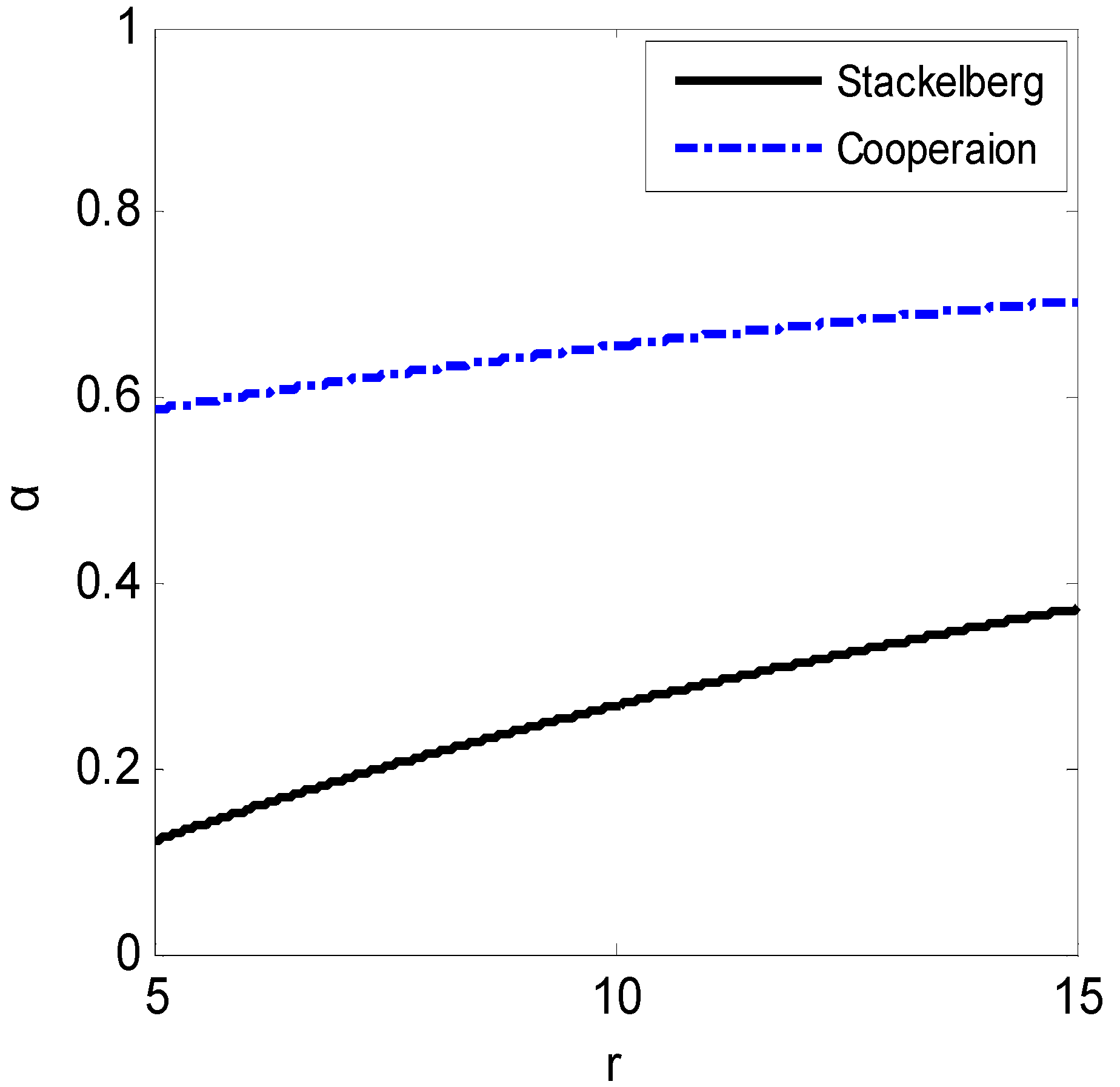
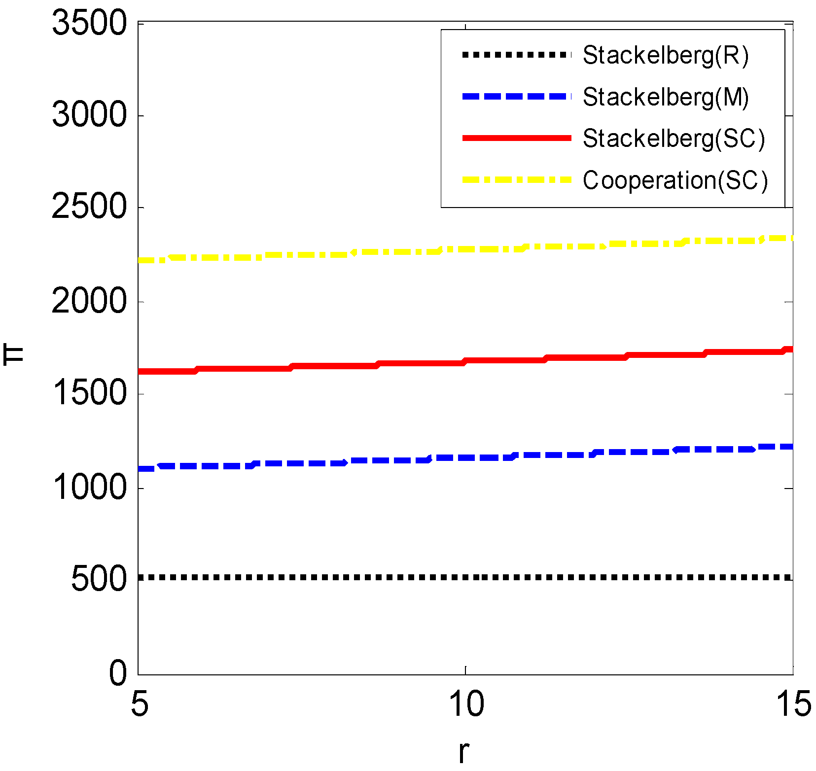
(1)

Impact of emission trading price r

Figure 2. α^* versus r.

Figure 2. α^* versus r.

Figure 3. ${{{\displaystyle \pi }}_1^R}^{\text{*}},{{{\displaystyle \pi }}_1^M}^{\text{*}},{{{\displaystyle \pi }}_1^{SC}}^{\text{*}},{{{\displaystyle \pi }}_{\text{2}}^{SC}}^{\text{*}}$ versus r.

Figure 3. ${{{\displaystyle \pi }}_1^R}^{\text{*}},{{{\displaystyle \pi }}_1^M}^{\text{*}},{{{\displaystyle \pi }}_1^{SC}}^{\text{*}},{{{\displaystyle \pi }}_{\text{2}}^{SC}}^{\text{*}}$ versus r.

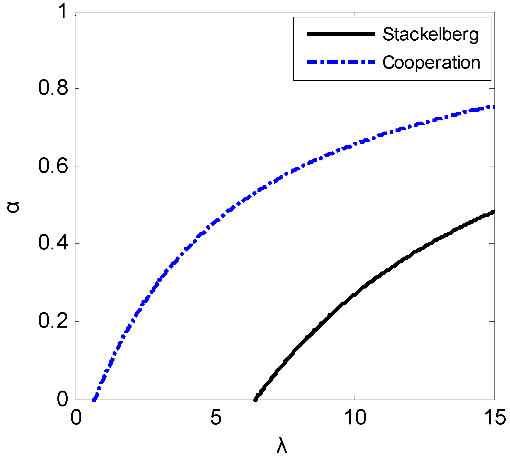
(2)

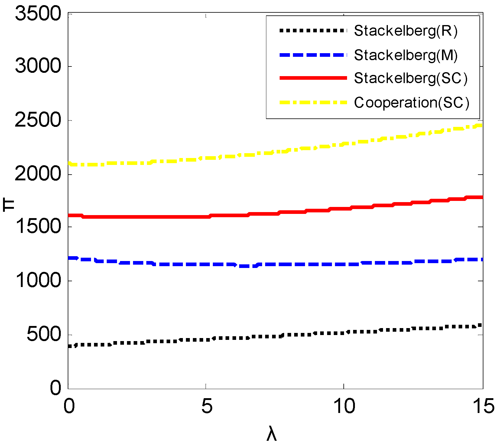
Impact of consumer preference coefficient of carbon λ

Figure 4. α^* versus λ.

Figure 4. α^* versus λ.

Figure 5. ${{{\displaystyle \pi }}_1^R}^{\text{*}},{{{\displaystyle \pi }}_1^M}^{\text{*}},{{{\displaystyle \pi }}_1^{SC}}^{\text{*}},{{{\displaystyle \pi }}_{\text{2}}^{SC}}^{\text{*}}$ versus λ.

Figure 5. ${{{\displaystyle \pi }}_1^R}^{\text{*}},{{{\displaystyle \pi }}_1^M}^{\text{*}},{{{\displaystyle \pi }}_1^{SC}}^{\text{*}},{{{\displaystyle \pi }}_{\text{2}}^{SC}}^{\text{*}}$ versus λ.

(3)

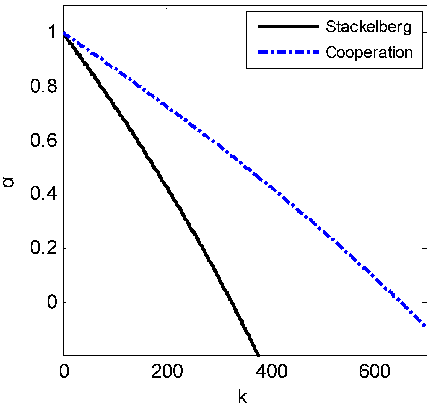
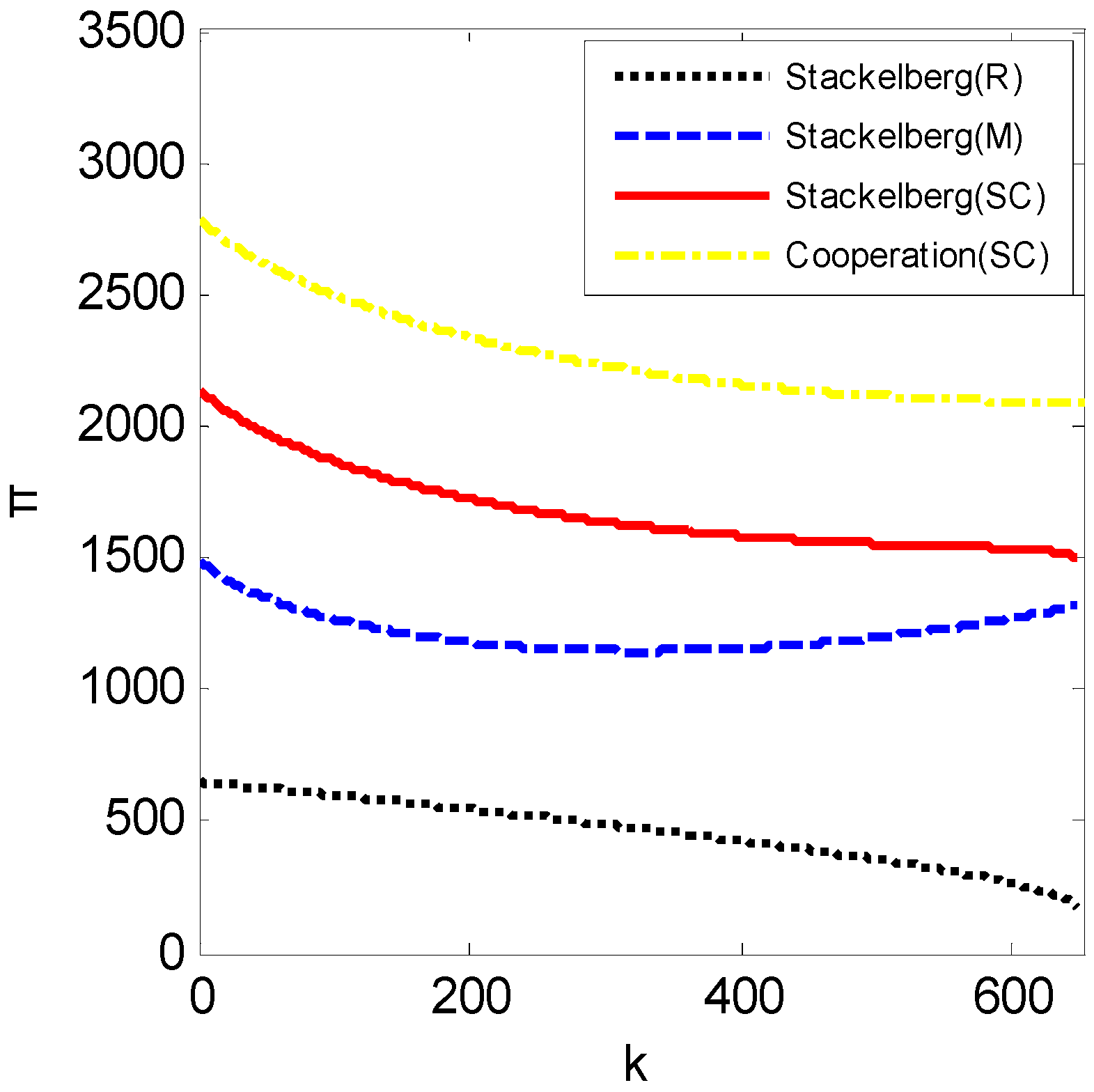
Impact of difficulty coefficient of emission reduction k

Figure 6. α^* versus k.

Figure 6. α^* versus k.

Figure 7. ${{{\displaystyle \pi }}_1^R}^{\text{*}},{{{\displaystyle \pi }}_1^M}^{\text{*}},{{{\displaystyle \pi }}_1^{SC}}^{\text{*}},{{{\displaystyle \pi }}_{\text{2}}^{SC}}^{\text{*}}$ versus k.

Figure 7. ${{{\displaystyle \pi }}_1^R}^{\text{*}},{{{\displaystyle \pi }}_1^M}^{\text{*}},{{{\displaystyle \pi }}_1^{SC}}^{\text{*}},{{{\displaystyle \pi }}_{\text{2}}^{SC}}^{\text{*}}$ versus k.

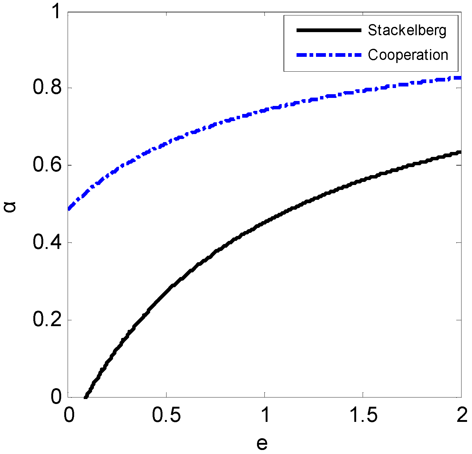
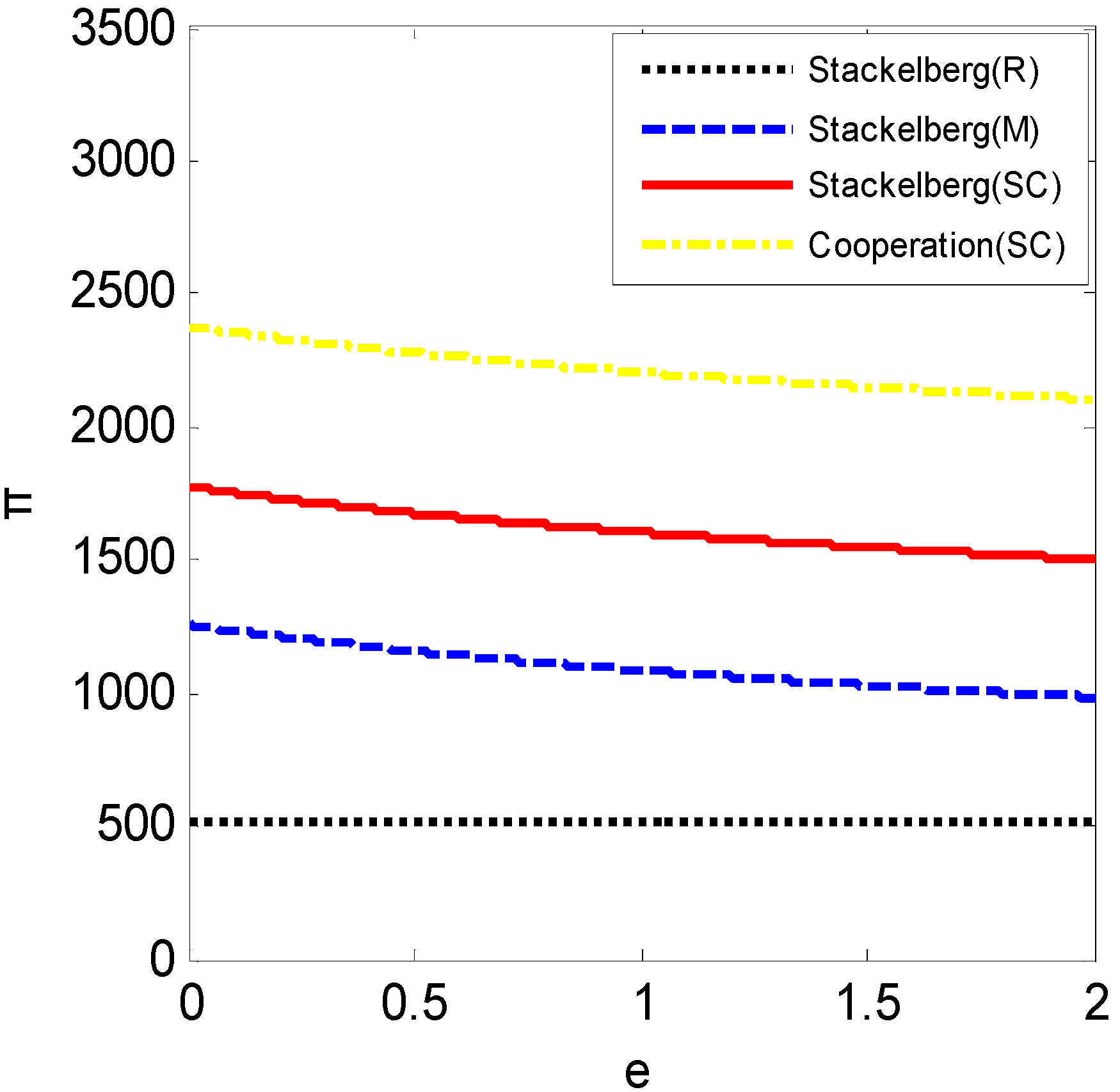
(4)

Impact of carbon emissions per unit product e₀

Figure 8. α^* versus e₀.

Figure 8. α^* versus e₀.

Figure 9. ${{{\displaystyle \pi }}_1^R}^{\text{*}},{{{\displaystyle \pi }}_1^M}^{\text{*}},{{{\displaystyle \pi }}_1^{SC}}^{\text{*}},{{{\displaystyle \pi }}_{\text{2}}^{SC}}^{\text{*}}$ versus e₀.

Figure 9. ${{{\displaystyle \pi }}_1^R}^{\text{*}},{{{\displaystyle \pi }}_1^M}^{\text{*}},{{{\displaystyle \pi }}_1^{SC}}^{\text{*}},{{{\displaystyle \pi }}_{\text{2}}^{SC}}^{\text{*}}$ versus e₀.

As shown in Figure 2, Figure 3, Figure 4, Figure 5, Figure 6, Figure 7, Figure 8 and Figure 9,

(i)

Emission trading price r, consumer preference coefficient of carbon λ, and carbon emissions per unit product e₀ have positive effects on the optimal percentage of emission reduction α^* in both the Stackelberg model and the cooperation model, while difficulty coefficient of emission reduction k shows a negative effect. Compared with the Stackelberg model, the manufacturer is more likely to invest in emission-reduction technology in the cooperation model.

(ii)

From the point of view of profit, in the Stackelberg model, emission trading price r and carbon emissions per unit product e₀ have no impact on the retailer’s profit, so that the manufacturer can increase its profit through reducing the percentage of emission reduction when facing a higher emission-reduction difficulty. However, this rule does not work given a lower emission-reduction difficulty. Besides, it is always more profitable for the whole supply chain when the manufacturer and the retailer maintain a cooperative relationship.

6.2. Numerical Results under a Contract of Revenue Sharing

An appropriately designed contract has important implications for not only the improvement of supply chain performance but also the strengthening of cooperative relationships between enterprises. In order to further study the influences of several exogenous parameters on the optimal percentage of emission reduction α^*, market demand, total emission, and profit under a revenue-sharing contract, we perform a sensitivity analysis and get several valuable managerial insights into environmental policy.

When the manufacturer plays the role of a Stackelberg leader, to get more profit, the contract parameter φ will be set infinitely close to the upper limit $1-\frac{{({\xi }_2+{\xi }_1{\alpha }_1)}^2}{4{({\xi }_2+{\xi }_1{\alpha }_3)}^2}$. Hence, we set $\phi =1-\frac{{({\xi }_2+{\xi }_1{\alpha }_1)}^2}{4{({\xi }_2+{\xi }_1{\alpha }_3)}^2}$ here.

As shown in Table 2, a rising emission trading price leads to a higher investment and less emissions. Although the investment cost is increased, manufacturers can get additional revenue as rewards through selling emission permits, thus increasing their profit. As for the retailer, since the gains and losses caused by the variation in emission trading price cancel each other out, its profit will not be affected. That is, stricter controls on the emission trading markets to avoid falling emission prices may help the government achieve its emission-reduction target and promote investment in emission-reduction technologies.

Table 2. Sensitivity of optimal result to r.

r	α2*	D2	e0D2(1 − α2*)	p	π3R*	π3M*	π3SC*
5	0.59	48.42	10.00	57.45	515.75	1707.54	2223.30
6	0.60	48.42	9.62	57.61	515.75	1717.74	2233.49
7	0.62	48.42	9.26	57.76	515.75	1728.30	2244.06
8	0.63	48.42	8.93	57.89	515.75	1739.21	2254.97
9	0.64	48.42	8.62	58.02	515.75	1750.44	2266.19
10	0.66	48.42	8.33	58.14	515.75	1761.96	2277.72
11	0.67	48.42	8.06	58.25	515.75	1773.77	2289.52
12	0.68	48.42	7.81	58.35	515.75	1785.83	2301.58
13	0.69	48.42	7.58	58.45	515.75	1798.14	2313.89
14	0.70	48.42	7.35	58.54	515.75	1810.67	2326.43
15	0.70	48.42	7.14	58.63	515.75	1823.43	2339.18
		→			→

Table 2. Sensitivity of optimal result to r.

r	α2*	D2	e0D2(1 − α2*)	p	π3R*	π3M*	π3SC*
5	0.59	48.42	10.00	57.45	515.75	1707.54	2223.30
6	0.60	48.42	9.62	57.61	515.75	1717.74	2233.49
7	0.62	48.42	9.26	57.76	515.75	1728.30	2244.06
8	0.63	48.42	8.93	57.89	515.75	1739.21	2254.97
9	0.64	48.42	8.62	58.02	515.75	1750.44	2266.19
10	0.66	48.42	8.33	58.14	515.75	1761.96	2277.72
11	0.67	48.42	8.06	58.25	515.75	1773.77	2289.52
12	0.68	48.42	7.81	58.35	515.75	1785.83	2301.58
13	0.69	48.42	7.58	58.45	515.75	1798.14	2313.89
14	0.70	48.42	7.35	58.54	515.75	1810.67	2326.43
15	0.70	48.42	7.14	58.63	515.75	1823.43	2339.18
		→			→

It can be inferred from Table 3 that both the manufacturer and the retailer stand to benefit from the increased consumer sensitivity toward emissions. However, from the perspective of a consumer, low-carbon products mean higher prices; namely, the consumer must pay more for the lower-carbon products. This finding has important implications for governments: they need to provide subsidies or tax exemptions to enterprises investing in emission-reduction technology in order to keep low prices.

Table 3. Sensitivity of optimal result to λ.

λ	α2*	D2	e0D2(1 − α2*)	p	π3R*	π3M*	π3SC*
5	0.45	45.77	12.50	56.50	428.92	1714.69	2143.61
6	0.51	46.30	11.36	56.75	442.90	1722.92	2165.82
7	0.56	46.83	10.42	57.06	459.04	1731.59	2190.63
8	0.59	47.36	9.62	57.39	477.03	1740.68	2217.71
9	0.63	47.89	8.93	57.75	496.65	1750.17	2246.81
10	0.66	48.42	8.33	58.14	517.70	1760.01	2277.72
11	0.68	48.95	7.81	58.54	540.06	1770.20	2310.27
12	0.70	49.47	7.35	58.96	563.61	1780.71	2344.32
13	0.72	50.00	6.94	59.39	588.24	1791.53	2379.77
14	0.74	50.53	6.58	59.83	613.89	1802.62	2416.51
15	0.76	51.05	6.25	60.28	640.49	1813.99	2454.48

Table 3. Sensitivity of optimal result to λ.

λ	α2*	D2	e0D2(1 − α2*)	p	π3R*	π3M*	π3SC*
5	0.45	45.77	12.50	56.50	428.92	1714.69	2143.61
6	0.51	46.30	11.36	56.75	442.90	1722.92	2165.82
7	0.56	46.83	10.42	57.06	459.04	1731.59	2190.63
8	0.59	47.36	9.62	57.39	477.03	1740.68	2217.71
9	0.63	47.89	8.93	57.75	496.65	1750.17	2246.81
10	0.66	48.42	8.33	58.14	517.70	1760.01	2277.72
11	0.68	48.95	7.81	58.54	540.06	1770.20	2310.27
12	0.70	49.47	7.35	58.96	563.61	1780.71	2344.32
13	0.72	50.00	6.94	59.39	588.24	1791.53	2379.77
14	0.74	50.53	6.58	59.83	613.89	1802.62	2416.51
15	0.76	51.05	6.25	60.28	640.49	1813.99	2454.48

The difficulty coefficient of emission reduction k has a negative effect on technology investment, as depicted in Table 4. The manufacturer prefers to reduce investment if it has technical limitations or cost limitations, even though that will result in less demand.

Table 4. Sensitivity of optimal result to k.

k	α2*	D2	e0D2(1 − α2*)	p	π3R*	π3M*	π3SC*
2.5	1.00	50.98	0.08	58.99	649.00	2135.19	2784.19
72.5	0.90	50.28	2.42	58.76	613.46	1944.72	2558.18
145	0.80	49.54	4.83	58.51	575.47	1841.46	2416.92
217.5	0.70	48.77	7.25	58.26	535.98	1778.72	2314.71
290	0.60	47.98	9.67	57.99	494.62	1743.66	2238.28
362.5	0.49	47.16	12.08	57.72	450.78	1730.62	2181.40
435	0.37	46.30	14.50	57.43	403.44	1736.96	2140.40
507.5	0.25	45.41	16.92	57.14	350.58	1762.32	2112.90
580	0.13	44.48	19.33	56.83	286.99	1810.26	2097.25
650	0.00	43.53	21.67	56.51	169.00	1923.26	2092.26

Table 4. Sensitivity of optimal result to k.

k	α2*	D2	e0D2(1 − α2*)	p	π3R*	π3M*	π3SC*
2.5	1.00	50.98	0.08	58.99	649.00	2135.19	2784.19
72.5	0.90	50.28	2.42	58.76	613.46	1944.72	2558.18
145	0.80	49.54	4.83	58.51	575.47	1841.46	2416.92
217.5	0.70	48.77	7.25	58.26	535.98	1778.72	2314.71
290	0.60	47.98	9.67	57.99	494.62	1743.66	2238.28
362.5	0.49	47.16	12.08	57.72	450.78	1730.62	2181.40
435	0.37	46.30	14.50	57.43	403.44	1736.96	2140.40
507.5	0.25	45.41	16.92	57.14	350.58	1762.32	2112.90
580	0.13	44.48	19.33	56.83	286.99	1810.26	2097.25
650	0.00	43.53	21.67	56.51	169.00	1923.26	2092.26

Since lower investment leads to more emissions, governments may consider providing manufacturers with technology investment subsidies or technical support. On the other hand, with increasing difficulty coefficient of emission reduction, the retailer’s profit and the supply chain’s profit both present a decreasing trend.

Although high-pollution firms are more willing to increase emission-reduction investment, little impact on demand and large amounts of emission make this investment less profitable, as shown in Table 5.

Table 5. Sensitivity of optimal result to e₀.

e0	α2*	D2	e0D2(1 − α2*)	p	π3R*	π3M*	π2SC*
0.0	0.48	48.42	0.00	56.42	517.70	1861.38	2379.08
0.2	0.57	48.37	4.63	57.33	517.70	1815.80	2333.50
0.4	0.63	48.34	7.92	57.98	517.70	1777.26	2294.97
0.7	0.70	48.47	9.81	58.49	517.70	1728.72	2246.43
0.9	0.73	48.43	11.70	58.85	517.70	1700.92	2218.62
1.1	0.75	48.40	13.22	59.14	517.70	1675.90	2193.60
1.3	0.78	48.38	14.48	59.37	517.70	1653.15	2170.86
1.6	0.80	48.46	14.97	59.55	517.70	1622.50	2140.21
1.8	0.82	48.44	15.88	59.72	517.70	1603.98	2121.68
2.0	0.83	48.42	16.67	59.86	517.70	1586.73	2104.43
					→

Table 5. Sensitivity of optimal result to e₀.

e0	α2*	D2	e0D2(1 − α2*)	p	π3R*	π3M*	π2SC*
0.0	0.48	48.42	0.00	56.42	517.70	1861.38	2379.08
0.2	0.57	48.37	4.63	57.33	517.70	1815.80	2333.50
0.4	0.63	48.34	7.92	57.98	517.70	1777.26	2294.97
0.7	0.70	48.47	9.81	58.49	517.70	1728.72	2246.43
0.9	0.73	48.43	11.70	58.85	517.70	1700.92	2218.62
1.1	0.75	48.40	13.22	59.14	517.70	1675.90	2193.60
1.3	0.78	48.38	14.48	59.37	517.70	1653.15	2170.86
1.6	0.80	48.46	14.97	59.55	517.70	1622.50	2140.21
1.8	0.82	48.44	15.88	59.72	517.70	1603.98	2121.68
2.0	0.83	48.42	16.67	59.86	517.70	1586.73	2104.43
					→

7. Conclusions

In the context of allowing emission trading and investment in emission-reduction technology, this paper presents three models for a two-stage supply chain under three scenarios, and analyzes the optimal investment decisions and pricing decisions in the hope of providing guidance to the government policy makers. The major findings are below:

(1)

With the emission reduction difficulty decreases or the consumer preference of low carbon increases, the equilibrium/optimal emission-reduction investment will increase.

(2)

The equilibrium/optimal emission reduction investment will increase with the carbon price increases while the emission quota allocated by the government will not alter the equilibrium/optimal emission reduction investment in the supply chain.

(3)

In a Non-cooperative Stackelberg setting, the equilibrium emission-reduction investment is less than that in Cooperative Model or Coordination Model. The equilibrium retail price in Stackelberg Model is higher than the optimal retail price in Cooperation Model or Coordination Model and this will make the supply chain suffer a loss in Non-cooperative Stackelberg setting.

(4)

The threshold for the difficulty coefficient of emission reduction to induce a positive emission reduction investment in the Stackelberg Model is lower than the threshold in Cooperation Model or Coordination Model.

(5)

Perfect coordination of the supply chain can be realized by a revenue-sharing contract.

From the consumer perspective, low-carbon products mean higher prices, so that subsidies or tax exemptions should be provided to keep low prices. Further, through controlling emissions-trading prices, strengthening publicity of energy conservation and emission-reduction, or providing technology investment subsidies, governments can promote investment in emission-reduction technologies and achieve their emission-reduction targets.

In future research, several studies can be carried out as extensions to the analysis of this paper. First, our study is limited to a two-stage supply chain consisting of a single emission-dependent manufacturer and a single retailer, so an extension study should take a multi-stage supply chain into consideration. Second, since our study is carried out under symmetric information, considering the integrity of systematic study, asymmetric cost information or asymmetric demand information should be incorporated into the problem setting.