Research on Urban Road Congestion Pricing Strategy Considering Carbon Dioxide Emissions

Abstract

Congestion pricing strategy has been recognized as an effective countermeasure in the practical field of urban traffic congestion mitigation. In this paper, a bi-level programming model considering carbon dioxide emission is proposed to mitigate traffic congestion and reduce carbon dioxide emissions. The objective function of the upper level model is to minimize the sum of travel costs and the carbon dioxide emissions costs. The lower level is a multi-modal transportation network equilibrium model. To solve the model, the method of successive averages (MSA) and the shuffled frog leaping algorithm (SFLA) are introduced. The proposed method and algorithm are tested through the numerical example. The results show that the proposed congestion pricing strategy can mitigate traffic congestion and reduce carbon emissions effectively.

1. Introduction

Urban road traffic congestion has been one of the worldwide urban problems (e.g., in some cities of China), which brings about many negative impacts. On the one hand, traffic congestion affects the efficiency and quality of life, such as lengthening travel time, increasing travel delays and resulting in traffic accidents. On the other hand, traffic congestion aggravates environmental pollution, such as reducing the use of fuel, increasing energy consumption and increasing pollutant emissions reduction. When traffic is congested, vehicles are often in the stop-and-go state, which leads to increased the carbon emissions. Previous studies [1] have shown that the emissions of motor vehicles are high in cases of stop-and-go traffic and in high-speed situations. As shown in Figure 1, the carbon dioxide emissions are lowest when the speed is between 64 km/h and 96 km/h. From the perspective of environmental protection, traffic congestion is a serious problem that needs to be solved.

Figure 1. Carbon emissions under different speed.

Figure 1. Carbon emissions under different speed.

Traffic congestion is caused by the unbalance of supply and demand, so the typical method of mitigating traffic congestion is to construct a transportation infrastructure, such as a road network. However, the development practices of many cities, both here and abroad, have shown that increasing the supply of transportation alone is not sufficient to meet the growth in transportation demand. In fact, congestion pricing strategy has been recognized as one of the most effective countermeasures of traffic demand management (TDM) to mitigate traffic congestion. Several regions (e.g., Singapore, London and Toronto) have implemented congestion pricing strategy for many years. Practice has proven that congestion pricing strategy can effectively transfer the car users to the public transportation and mitigate traffic congestion.

Several articles have studied the congestion pricing strategy. The concept of congestion pricing [2,3] was put forward on the basis of marginal cost pricing principle of economics. Several articles have studied the congestion pricing strategy. The concept of congestion pricing [2,3] was put forward on the basis of marginal cost pricing principle of economics. The major congestion pricing models are the static models (Walters [4], Dafermos and Sparrow [5], Dafermos [6], Yang and Huang [7]) and the dynamic models (Wie and Tobin [8], Yang and Hai-Jun [9], Arnott et al. [10]). Some scholars (Walters [4], Yang and Huang [7], Yildirim and Hearn [11]) proposed each link of the network should be charged according to the theory of marginal cost pricing. However, the high cost makes the congestion pricing strategy have low public acceptance. Then, some scholars proposed the optimal system (Verhoef [12], Yang and Zhang [13]). These papers regarded parts of the roads or links as tolled objects, and few guaranteed that the total carbon emissions would decrease after implementing the congestion pricing strategy.

The typical aim of traffic congestion pricing strategy is to minimize the total travel time of the entire transportation system. The reduction of carbon dioxide emissions has been another important aim of traffic congestion pricing strategy, as haze has become a more and more serious problem. Due to the difficulty of calculating carbon emissions, few studies investigate traffic congestion pricing considering carbon emissions. The models used for calculating carbon dioxide emissions on the road can be divided into the micro-scale model and the macro-scale model. The micro-scale model (e.g., Comprehensive Modal Emissions Model, CMEM) calculates the amount of instantaneous emission [14,15] using the driving cycles of vehicles, vehicle data, road gradient and so on. Estimating the exact amount of carbon dioxide emission with detailed input data is the advantage of this model, but it is impossible to collect the exact driving cycle data of all vehicles on the road. The macro-scale model (e.g., COPERT, MOBILE, EMFAC) uses emission factors (EFs) and vehicle kilometers traveled (VKT) per average speed of different vehicle types to calculate the amount of emission per link unit [14]. The macro-scale model can calculate the total carbon dioxide emission of all vehicles within the given link on the base of average speed, so it is more appropriate than the micro-scale model. However, the average speed model cannot reflect driver behavior and road characteristics, Ryu et al. [16] verified the accuracy of the average speed model, analyzed the cause of errors affecting the accuracy and developed a model that can improve the accuracy. In this paper, the corrected average speed model [16] is introduced to calculate the total carbon dioxide emission.

Due to the difficulty of calculating carbon emissions, few studies investigate traffic congestion pricing considering carbon emissions. Naguemey et al. [17,18,19] presented a multimodal traffic network equilibrium model with emission pollution permits and paradoxes on the road network with zero emission links. Almodóvar et al. [20] presented to mitigate traffic congestion in the form of optimal CO₂ emission taxes for private transport. Li et al. [21] proposed environmentally sustainable toll design for congested road networks with uncertain demand. Hensher [22] assessed the influence on CO₂ of a number of “at source” and “mitigation” instruments such as improvements in fuel efficiency, a carbon tax, variable user charges, and improvements in public transit. Nicolas and David [23] analysed CO₂ emissions caused by passenger transport in France. Ubeda et al. [24] proposed the crowded conditions of road can affect carbon emissions, and calculated carbon emissions through travel distance, assuming fuel combust completely. In this paper, the corrected average speed model [16] is introduced to calculate the total carbon dioxide emission, which is easier than micro-scale models. It has good generalization and can apply a wide range of practical problems.

In this paper, the average speed model is proposed to calculate carbon emissions. Then, a bi-level programming model considering carbon dioxide emission is proposed to mitigate traffic congestion and reduce carbon dioxide emissions. Moreover, there schemes is analysed in this paper. Scheme 1 does not implement traffic congestion pricing; Scheme 2 only considers the congestion into the objective function; Scheme 3 considers both the congestion and carbon emissions costs into the objective function. The results shows that the scheme proposed in this papper can mitigate traffic congestion and reduce carbon emissions more effectively than the other two schemes. This paper provides a reference for the future congestion pricing strategy in many cities and has practical significance.The rest of this paper is organized as follows. In Section 2, problem formulation is introduced. The lower level model of the bi-level programming model and the upper level model of the bi-level programming model is proposed. In Section 3, to solve the model, the method of successive averages (MSA) and the shuffled frog leaping algorithm (SFLA) are introduced. In Section 4, the numerical example is introduced. The result shows that the traffic congestion pricing strategy will improve the efficiency of both public and private transport, while at the same time it is able reduce carbon emissions. Finally, some conclusions and direction for future research are provided in Section 5.

2. Model Development

With traffic congestion more serious, people pay more and more attention on the traffic management. The relevant departments begin to charge a form of congestion pricing, if they go through the crowded regions or crowded links. Actually, the essence of congestion pricing is a process of traffic reassignment, and it can balance the traffic supply and traffic demand in a certain period of time. Congestion pricing can make full use of the road resource and ensure the efficient operation of the urban traffic system. Meanwhile, the fees can be used to subsidize public transport, which can improve the public transport service level and the public transport attraction.

Urban congestion pricing is a typical bi-level programming problem. The upper level traffic administrative department hopes to ensure optimal system efficiency through congestion pricing. The lower level traveler wants to reach its destination through the minimum cost or the minimum time by adjusting the path. Upper traffic managers focus on system efficiency, whereas the lower travelers only care about personal interests. Upper management needs to find a pricing scheme for the urban traffic network under the equilibrium state.

2.1. Assumptions

The following assumptions are introduced to simplify the construction and the calculation of the bi-level programming model:

There are only two travel modes, car and bus.

Assume one person per car and all buses of the same type, whose capacity can accommodate B passengers.

All the travelers can obtain traffic network information accurately; the traffic demand is constant and no demand response.

Do not take toll revenues and fare revenues into account. In China, most public transport operator is publicly owned and government subsidies are high. For example, the government subsidy of Dalian public transport operator is 2.5 billion. Therefore, Compared with toll revenues and fare revenues, we are more concerned with how to mitigate traffic congestion and reduce carbon emissions.

2.2. The Bi-Level Programming Model

A summary of the bi-level programming model construction is as follows. First, perform modal split and traffic assignment from the perspective of traveler. And the lower level model is proposed. Then, minimize the sum of the road users’ travel costs and the carbon dioxide emissions costs from the perspective of the traffic department; the upper level model is proposed. Finally, implement to mitigate traffic congestion and reduce carbon emissions through iteration.

2.3. The Lower Level Model: Multi-Modal Transportation Network Equilibrium

Urban road congestion pricing strategy has widely been recognized as an effective countermeasure in the practical field of urban traffic congestion mitigation. The congestion pricing aims to transfer the traffic flow from the crowded roads to clear roads, which is a process of traffic reassignment. In the traffic assignment, all the OD demand is distributed to the multi-modal transportation network.

If travelers know the information of the transportation network accurately, they will choose the shortest path or the minimal general travel costs path obviously. In this paper, it is assumed that travelers have the choice between two travel modes in the transportation network, car and bus transit. Travelers’ mode choice depends on the general travel costs of two modes. Travelers’ general travel costs by car primarily consist of travel time and congestion pricing. Travelers’ general travel costs by bus primarily consist of travel time and bus fares. The traveler’s choice between two modes is based on a logit function split. However, within the same mode, the travelers choose their path based on user equilibrium principle of general travel costs. The multi-modal transportation network equilibrium analysis attempts to solve a combined model with modal split and user equilibrium based on the travelers’ general travel costs.

2.3.1. Modal Split Based on a Logit Function

Consider a road transportation network (V, A), where V and A denote the sets of nodes and links, respectively. Let Q_rs denote the total travel demand from origin r to destination s, where (r, s) ∈ RS ⊂ V × V. Let K_rs denote the path set from the origin r to the destination s, where k ∈ K_rs, The link flow can be written as follows:

$$x_a^c={\displaystyle \sum _{(r,s)\in RS}{\displaystyle \sum _{k\in K_{\text{rs}}}{\delta }_{ak}^c}}\times f_k^c,\forall a\in A$$

(1)

$$x_a^b={\displaystyle \sum _{(r,s)\in RS}{\displaystyle \sum _{k\in K_{\text{rs}}}{\delta }_{ak}^b}}\times f_k^b,\begin{array}{cc}& \forall a\in A\end{array}$$

(2)

where $x_a^c$ and $x_a^b$ denote the link flow of travelers by car and bus for $\forall a\in A$, respectively. ${\delta }_{ak}^c({\delta }_{ak}^b)$ denote the relationship between path and link; ${\delta }_{ak}^c({\delta }_{ak}^b)=1$ if the path k passes link a; otherwise ${\delta }_{ak}^c({\delta }_{ak}^b)=0$.

To facilitate analysis, assume one person per car and all buses of the same type, whose capacity can accommodate $B$ passengers. The actual travel time of travelers by car and bus on link a can be written by a BPR (Bureau of Public Road) function as follow:

$$t_a^c=t_{a0}^c\times \left[1+{\alpha }^c{\left(\frac{x_a^c+K\times \raisebox{1ex}{$X_a^b$}\!\left/ \!\raisebox{-1ex}{$B$}\right.}{C_a}\right)}^{{\beta }^c}\right],\begin{array}{cc}& a\in A\end{array}$$

(3)

$$t_a^{\text{b}}=t_{b0}^b\times \left[1+{\alpha }^b{\left(\frac{x_a^c+K\times \raisebox{1ex}{$X_a^b$}\!\left/ \!\raisebox{-1ex}{$B$}\right.}{C_a}\right)}^{{\beta }^b}\right],\begin{array}{cc}& a\in A\end{array}$$

(4)

where $t_{a0}^c$ and $t_{a0}^b$ denote the travel time of travelers by car and bus on link $a$ in a free circumstance, respectively; ${\alpha }^c、{\alpha }^b、{\beta }^c、{\beta }^b$ denote the corrected BPR parameters; denote the vehicle conversion coefficient; $C_a$ denotes the actual capacity of link $a$.

Economic assessments of externalities from road travel include the costs of air pollution emissions, noise, space consumption, fuel consumption, vehicle maintenance, road maintenance, and other dimensions (Maibach et al. [25]; Parry et al. [26]). Time is usually the largest single cost component, but the estimation of other costs is important for the development of roadway pricing systems that aim to internalize the external costs of transportation [27]. In this paper, travelers’ total travel costs by car primarily consist of travel time and congestion pricing. Travelers’ total travel costs by bus primarily consist of travel time and bus fares. $C_k^c$ and $C_k^b$ represent the total travel costs by car and bus on the path $K$ from the origin $r$ to the destination $s$, respectively, and can be written as follows:

$$C_k^c={\gamma }^c\times {\displaystyle \sum _{a\in A}{\delta }_{ak}^c\times t_a^c+{\displaystyle \sum _{a\in A}{\delta }_{ak}^c\times u_a}},\begin{array}{cc}& \forall k\in K_{rs},(r,s)\in RS\end{array}$$

(5)

$$C_k^b={\gamma }^b\times {\displaystyle \sum _{a\in A}{\delta }_{ak}^b\times t_a^b+m_k},\begin{array}{cc}& \forall k\in K_{rs},(r,s)\in RS\end{array}$$

(6)

where ${\mu }_{\mapsto }$ = the congestion pricing on the link $a$; $m_k$ = the bus fares on the path $k$; ${\gamma }^{\Updownarrow }$, ${\gamma }^{\updownarrow }$ = value of time of travelers by car and bus, respectively.

$$C_{rs}^c=Min\left\{C_k^c|k\in K_{rs}\right\},\begin{array}{cc}& \forall (r,s)\in RS\end{array}$$

(7)

$$C_{rs}^b=Min\left\{C_k^b|k\in K_{rs}\right\},\begin{array}{cc}& \forall (r,s)\in RS\end{array}$$

(8)

where $C_{rs}^c$, $C_{rs}^b$ = the total intuitively minimal travel costs by car and bus on the path from the origin $r$ to the destination $s$, respectively.

According to the principle of utility maximization, travelers will choose the shortest path or the minimal general travel costs path. $P_{rs}^b$. represents the probability of choosing bus from the origin $r$ to destination $s$. The value of $P_{rs}^b$ is equal to the probability of bus costs considered to be the least.

The utility function of modal split is considered as the negative path costs, $V_k^c=-\theta \times C_k^c,V_k^b=-\theta \times C_k^b$, where $\theta$ is the empirical parameter to describe the randomness of traffic network. $\theta$ reflects the travelers’ familiarity of the traffic network. The value of $\theta$ and perceptual error is inversely proportional to the size. When $\theta$ is high, the majority of people chooses the shortest path.

According to the principle of utility maximization, the probability of choosing bus $P_{rs}^b$ can be written as follow:

$$\begin{array}{l}{P}_{rs}^b=\frac{\exp (V_{rs}^b)}{\exp (V_{rs}^b)+\exp (V_{rs}^c)}=\frac{\exp (-\theta \times C_{rs}^b)}{\exp (-\theta \times C_{rs}^b)+\exp (-\theta \times C_{rs}^{\text{c}})+\exp (-\theta \times \varphi )}\\ =\frac{1}{1+\exp [\theta \times (C_{rs}^b-C_{\text{rs}}^c-\varphi )]},\begin{array}{cc}& \forall k\in K_{rs},(r,s)\in RS\end{array}\end{array}$$

(9)

where $\varphi$ is empirical parameter, and $\varphi =0$ means it has no impact on mode choice. Because the modal split is based on the logit function split of general travel path costs, the travel demand of the two modes $q_{rs}^b$ and $q_{rs}^c$ can be formulated as:

$$q_{rs}^b=Q_{rs}\times p_{rs}^b=\frac{Q_{rs}}{1+\exp [\theta \times (C_{rs}^b-C_{\text{rs}}^c-\varphi )]},\begin{array}{cc}& \forall k\in K_{rs},(r,s)\in RS\end{array}$$

(10)

$$q_{rs}^c=Q_{rs}-q_{rs}^b,\begin{array}{cc}& \forall k\in K_{rs},(r,s)\in RS\end{array}$$

(11)

2.3.2. The Lower Level Model Based on Beckman-UE Model

If travelers know the information of the transportation network accurately, travelers choose the paths with minimal travel costs in traffic network (V, A). The user equilibrium state is reached when the total travel costs of all paths for the same origin-destination (OD) pair are equal and the total travel costs of all unused paths are not lower than total travel costs of used paths. Based on the preceding analysis, a multi-modal transportation network equilibrium model can be confirmed as follows:

$$Min{\displaystyle \sum _{(r,s)\in RS}{\displaystyle \sum _{k\in K_{\text{rs}}}\left[{\displaystyle {\int }_0^{f_k^c}{C}_k^c(w)}dw+{\displaystyle {\int }_0^{f_k^b}{C}_k^b(w)}dw\right]}}$$

(12)

$$s.t.{\displaystyle \sum _{k\in K_{rs}}{f}_k^c=q_{rs}^c},\begin{array}{cc}& \forall (r,s)\in RS\end{array}$$

(13)

$${\displaystyle \sum _{k\in K_{rs}}{f}_k^b=q_{rs}^b},\begin{array}{cc}& \forall (r,s)\in RS\end{array}$$

(14)

$$f_k^c\ge 0$$

(15)

$$f_k^b\ge 0$$

(16)

subject to: Equations (1)–(11).

2.4. The Upper Level Model: Cost Optimization of the Traffic Network

Considering the deterministic travel demand situation, the total general costs of the multi-modal transportation system can be considered to consist of two parts. The first part is the sum of travelers total travel costs in the multi-modal transportation network. The second part is the total costs of carbon dioxide emissions. In 2008, road emissions accounted for 80% of the total emission in the transportation sector, which has since then increased continuously [28]. In particular, carbon dioxide (CO₂) emissions on roads in urban centers substantially affect global warming.

2.4.1. Carbon Emissions Model Based on Average Speed

Because of the dramatic growth of car ownership, traffic congestion is becoming increasingly prominent. Congestion traffic can make a negative effect to our environment, such as reducing the fuel efficiency and increasing pollutant emissions reduction. Previous studies have shown that the emissions of motor vehicles are highest in cases of stop-and-go traffic and in high-speed situations. Obviously, the road motor vehicles will inevitably be in the stop-and-go state when the traffic is congestive. It is important to quantify CO2 emissions in terms of the link unit in order to reduce these emissions on the roads. In order to estimate emissions-related congestion externalities, modeled emissions rates must be at least a function of speed [29]. In this study, the average speed model [30] is applied to estimate CO2 emissions. In order to carbon emissions per link unit in the urban center, the emission factor $E{F}_a^c$ and $E{F}_a^b$ are required. The calculation for carbon emissions per link unit can be shown below in Equations (17) and (18).

$${\text{g}}_a^c=x_a^c\times l_a\times E{F}_a^c$$

(17)

$${\text{g}}_a^b=x_a^b\times l_a\times E{F}_a^b$$

(18)

where $g_a^c$ and $g_a^b$ are the carbon emissions (g/T) on link $a$ by car and bus, respectively. $l_a$ is the length of link $a$. $x_a^c$ and $x_a^b$ are the traffic flow on link $a$ by car and bus, respectively; $E{F}_a^c$ (g/km⁻¹) and $E{F}_a^b$ (g/km⁻¹) represent emission factors by car and bus on link $a$, respectively.

Ryu et al. [14] formulized the emission factors of different vehicle type with different fuel type, when T = 15 min. In this paper, cars are considered as light duty gasoline vehicles (LDGV) and buses are considered as heavy duty diesel vehicles (HDDV). For the accelerating speed, fuel consumption is affected and the carbon emission is high. The carbon emissions model can be written as follow with a division of 65 km/h.

$$E{F}_a^c=\{\begin{array}{c}1313.7{(v_a^c)}^{-0.6},\begin{array}{cc}& 0<v_a^c<65km/h\end{array}\\ 0.5447v_a^c+78.746,\begin{array}{cc}& v_a^c\ge 65km/h\end{array}\end{array}$$

(19)

$$E{F}_a^b=\{\begin{array}{c}1555.5{(v_a^b)}^{-0.578},\begin{array}{cc}& 0<v_a^b<65km/h\end{array}\\ 0.0797v_a^b+144.19,\begin{array}{cc}& v_a^b\ge 65km/h\end{array}\end{array}$$

(20)

where $v_a^c$ and $v_a^b$ are the average speed on link $a$ by car and bus, respectively, where ${\text{v}}_a^c=\frac{l_a}{t_a^c},\forall a\in A$ and ${\text{v}}_a^b=\frac{l_a}{t_a^b},\forall a\in A$.

Congestion causes a lot of stop-and-go traffic, which increases waiting queues, the time of the accelerating speeds, and signals. For idle time or the accelerating speed, fuel consumption is affected and the carbon emission is high. However, the average speed model was unable to reflect such traffic behaviors, so the result of the average speed model was a lower estimation of emissions than the instantaneous emission model.

The results of an analysis of the average speed model and the instantaneous emissions model showed that traffic congestion caused a bigger error, so Byu et al. [30] revised the value of the average speed model during congestion. The sum of the accelerating speeds in the range 20–40 km/h was rather high but its error in emissions was low, which was affected by acceleration and deceleration without stops. However, the error of the range of 20 km/h and lower was clearly large. In this paper, a corrected average speed model [30] is introduced as follow:

$$g_a^c=\{\begin{array}{c}1.1767(x_a^c\times l_a)\times E{F}_a^c-2.8044,\begin{array}{cc}& 0<v_a^c<20km/h\end{array}\\ x_a^c\times l_a\times E{F}_a^c,\begin{array}{cc}& v_a^c\ge 20km/h\end{array}\end{array}$$

(21)

$$g_a^b=\{\begin{array}{c}1.1767(x_a^b\times l_a)\times E{F}_a^b-2.8044,\begin{array}{cc}& 0<v_a^b<20km/h\end{array}\\ x_a^b\times l_a\times E{F}_a^b,\begin{array}{cc}& v_a^b\ge 20km/h\end{array}\end{array}$$

(22)

2.4.2. The Upper Level Model

Traffic managers focus on cost optimization and system efficiency. Considering the deterministic travel demand situation, the total general costs of the multi-modal transportation system can be considered to consist of two parts. The first is the sum of travelers total travel costs in the multi-modal transportation network. The second is the total costs of carbon dioxide emissions. The congestion pricing can be calculated by follow function:

$$Min{\displaystyle \sum _{(r,s)\in RS}(C_{rs}^c{q}_{rs}^c+C_{rs}^b{q}_{rs}^b)}+{\gamma }_g{\displaystyle \sum _a(g_a^c\times \raisebox{1ex}{$t_a^c$}\!\left/ \!\raisebox{-1ex}{$T$}\right.+g_a^b\times \raisebox{1ex}{$t_a^b$}\!\left/ \!\raisebox{-1ex}{$T$}\right.)}$$

(23)

$$\text{subject to }0\le u_a\le u_a^{\max },\begin{array}{cc}& \forall a\in A\end{array}$$

(24)

subject to: Equations (1)–(11) and Equations (17)–(22). where ${\gamma }_g$ is the conversion parameter of carbon emissions costs; ${\mu }_a=$ the congestion pricing on the link $a$; ${\mu }_a^{\max }=$ maximal congestion pricing on the link a.

3. Solution Algorithm

The bi-level programming problem is a NP problem, and there is not an effective global algorithm up to now. Even if both the upper and the lower level model are convex programming problems, the bi-level programming problem is not likely to be a convex programming problem. So the solution of algorithm might be a local rather than a global optimal solution. The shuffled frog leaping algorithm (SFLA) is more likely to get global optimal solution, which has strong robustness and global optimization capability. This paper introduces the method of successive averages (MSA) and the shuffled frog leaping algorithm (SFLA) to solve the bi-level programming problem.

3.1. Algorithm 1. The Method of Successive Averages (MSA) of the Lower Level Model

The lower level of the bi-level programming model is a multi-modal transportation network equilibrium model. To solve the lower level model, the method of successive averages (MSA) is introduced. In iterations, firstly, it is necessary to evaluate which travel mode has a lower demand than the demand that it can gain by a logit split function for each OD pair. Secondly, the path must be found that currently has minimal general travel costs for the mode, and the auxiliary path flows must be determined by loading all OD demand to that path. Finally, the auxiliary path flows are loaded into current path flows using “MSA”.

Input: Transportation network $(V,A)$, capacities $C_a,a\in A$, traffic demand $Q_{rs},(r,s)\in RS$ and split capacities $\theta ,\varphi$; related parameters by bus: $B,K,t_{a0}^b,{\alpha }^b,{\beta }^b,{\gamma }^b,m_k,a\in A,k\in K_{rs},(r,s)\in RS$ related parameters by car: $t_{a0}^c,{\alpha }^c,{\beta }^c,{\gamma }^c,a\in A,k\in K_{rs},(r,s)\in RS$, convergence precision $\epsilon$ and iteration number $N$;

Output: Bus related $q_{rs}^b,e_{rs}^b,f_k^b,k\in K_{rs},(r,s)\in RS$; Car related $q_{rs}^c,e_{rs}^c,f_k^c,k\in K_{rs},(r,s)\in RS$.

Step 0: Initialization. For $k\in K_{rs},(r,s)\in RS,f_k^{c(0)}=0;f_k^{b(0)}=0;n=0;$

Step 1: Perform an all-or-nothing assignment. For $k\in K_{rs},(r,s)\in RS$, calculate $C_k^c$ using Equation (5); For $k\in K_{rs},(r,s)\in RS$, calculate $C_k^b$ using Equation (6); Calculate $C_{rs}^c,C_{rs}^b,t_a^c,t_a^b$ using Equations (3), (4), (7) and (8);

Step 2: Calculate additional flow path. Calculate additional flow path $F_k^{b(n)}$ and $F_k^{c(n)}$ using Equation (12);

Step 3: Update path flow using.

For $k\in K_{rs},(r,s)\in RS,f_k^{b(n+1)}=f_k^{b(n)}+\frac{1}{n}(F_k^{b(n)}-f_k^{b(n)}),\forall k\in K_{rs},n\ge 1$, calculate auxiliary path flows $f_k^{b(n+1)}$; For $k\in K_{rs},(r,s)\in RS,f_k^{c(n+1)}=f_k^{c(n)}+\frac{1}{n}(F_k^{c(n)}-f_k^{c(n)}),\forall k\in K_{rs},n\ge 1$, calculate auxiliary path flows $f_k^{c(n+1)}$;

Step 4: Check convergence. If $n\ge N$ or $1<n<N$, $\frac{\sqrt{{\displaystyle \sum _{k\in K_{rs}}{(f_k^{b(n+1)}-f_k^{b(n)})}^2}}}{{\displaystyle \sum _{k\in K_{rs}}{f}_k^{b(n)}}}<\epsilon$ and $\frac{\sqrt{{\displaystyle \sum _{k\in K_{rs}}{(f_k^{c(n+1)}-f_k^{c(n)})}^2}}}{{\displaystyle \sum _{k\in K_{rs}}{f}_k^{c(n)}}}<\epsilon$. Then go to Step 5; otherwise, let $n=n+1$, go to Step 1;

Step 5: Calculate $q_{rs}^b,q_{rs}^c$ using Equations (10) and (11)

3.2. Algorithm 2. The Shuffled Frog Leaping Algorithm (SFLA) of the Upper Level Model

3.2.1. Shuffled Frog Leaping Algorithm

Shuffled frog leaping algorithm (SFLA) was developed by Eusuff and Lansey [31]. It is a meta-heuristic optimization method which combines the benefits of genetic-based memetic algorithm (MA) and the social behavior-based particle swarm optimization (PSO) algorithm. The meme is a kind of information body for distribution, reproduction, and exchange by infecting the thought of human or animal. The most obvious characteristics of meme algorithm is that memes can share and exchange experience, knowledge and information between memes or in each meme by a local search method in the process of evolution.

In the Shuffled frog leaping algorithm, the population consists of the frogs with similar structure. Each frog represents a solution. The entire population is divided into many subgroups. Each subgroup performs local search. They can communicate with each other and improve their memes among local individuals. After a pre-defined number of memetic evolution steps, information is passed between memeplexes in a shuffling process. Shuffling ensures that the cultural evolution towards any particular interest is free from bias. The local search and the shuffling processes alternate until satisfying the stopping criteria.

For the problem of D dimensions, a frog is thought as $F_i$ = (f_i1, f_i2,…, f_iD). The algorithm first randomly generates F frogs as the initial population, ranks them in descending order according to the fitness of each frog. Then the entire population is divided into m subgroups, and each subgroup contains n frogs. From the initial population, the first frog is selected in the first subgroup, the second frog is selected in the second group, until the m^th frog is selected in the m^th subgroup. Then, the (m + 1)^th frog is selected in the first subgroup. Repeat the process, until all frogs are distributed.

In each subgroup, the frog with the best fitness and the worst fitness are denoted as F_b and F_w, respectively. While, in the total population, the frog with the best fitness is denoted as F_g. The main work of SFLA is to update the position of the worst-performing frog through iterative operation in each subgroup. Its position is improved by learning from the best frog of the sub-memeplex or its own population and position. In each subgroup, the new position of the worst frog is updated according to the following equation.

$$S=\{\begin{array}{c}\min \{\mathrm{int}[rand(F_b-F_w)],S_{\max }\},F_b-F_w\ge 0\\ \max \{\mathrm{int}[rand(F_b-F_w)],-S_{\max }\},F_b-F_w<0\end{array}$$

(25)

$$F_w=F_w+S$$

(26)

Equation (25) is used to calculate the updating step vector S, S_max means the maximum step size allowed to change by frog individual. Rand ( ) is the random number between 0 and 1. Equation (26) updates the position of F_w. If a better solution is attained it will replace the worst individual. Otherwise, F_g will instead of F_b. Then, recalculate Equation (25). If it still cannot get a better solution, new explanations, generated randomly, will replace the worst individual. Repeat until a predetermined number of iterations, and complete the round local search of various subgroups. Then all subgroups of the frogs are re-ranked in mixed sort, and divided into sub-group to the next round of local search.

3.2.2. Coding

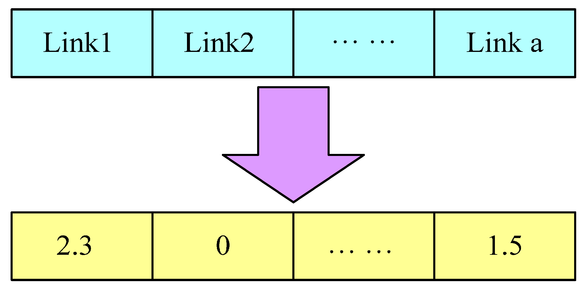
In this paper, a multi-dimensional code format based on real numbers is introduced. Each gene value of the individual is in a range of a floating point number. The coding length of individuals is equal to the number of links. In this paper, each coding can be shown as in Figure 2. The traffic congestion pricing of each link generates randomly within the scope of a floating point number.

Figure 2. Example of coding.

Figure 2. Example of coding.

3.2.3. The Process of Algorithm

The general structure of SFLA can be described as follows:

Step 0: Input population size, the maximum number of iterations $J$. Define the chromosome segment and the code rule of chromosome.

Step 1: Initial population. Randomly generate an initial population $U_a(0)$ with F individuals (F = m × n), according to the maximal congestion pricing and population size. For the D dimension optimization problem, the individuals of the population are D dimension variables and it represents the frog’s current position. Calculate $q_{rs}^c,q_{rs}^b,C_{rs}^c,C_{rs}^b,f_k^c,f_k^b,t_k^c,t_k^b$ using Algorithm 1; then calculate current minimal transportation system costs using Equation (23), which represented by $E$; let $j=0$;

Step 2: For $U_a\in U_a(j)$, calculate their fitness function $F_i=\left|E_i(U_a)-\{E(U_a)\},U_a\in U_a(j)\right|$, which is used to determine if the performance of the position is good. Then note individuals in descending order according to the fitness of each frog.

Step 3: Divide the population into m subpoplations: Y₁, Y₂, ..., Y_m. Each sub population contains n frogs.

Step 4: In each subgroup, with its evolution, the positions of individuals have been improved. The following steps are the process of the subgroup local search.

Step 4.0: In each sub population, compute F_b and F_w, respectively. Set i_m = 0. i_m represents the number of the sub population, which is from 0 to M. Set i_n= 0. i_n represents the number of evolution which is from o to N (the maximum evolution iteration in each sub population).

Step 4.1: i_m = i_m + 1

Step 4.2: i_n = i_n + 1

Step 4.3: Try to adjust the position of the worst frog using Equation (25) and Equation (26). If a better solution is attained, it will replace the worst individual. Otherwise, F_g will instead of F_b. Then, recalculate Equation (25). If it still cannot get a better solution, new individual generated randomly will replace the worst individual.

Step 4.4: If i_n < N, then do Step 4.2

Step 4.5: If i_m < M, then do Step 4.1

Step 5: Implementation mix operations. After each subgroup carrying out a certain number of meme evolution, merge each subgroup Y₁, Y₂, ..., Y_m. to X, descend X again and updates the best frog F_g in the populations.

Step 6: Stop check. If the iterative termination conditions meet, then stop, calculate $q_{rs}^c,q_{rs}^b,C_{rs}^c,C_{rs}^b,f_k^c,f_k^b,t_k^c,t_k^b$ using Algorithm 1; then calculate current minimal transportation system costs using Equation (23). Otherwise, do Step 3 again.

4. Numerical Example

4.1. The Traffic Network of Numerical Example

As shown in Figure 3, to illustrate the proposed model, an urban road network based on Nguyen and Dupuis [32] is constructed. There are two travel modes in Figure 3, car and bus. The car network is shown in solid line, and the bus network is shown in dashed line. c_i represents the link i of the car network, and bij represents the link j on the path i of the bus network. For example, b12 represents the second link on Path 1.

Figure 3. Numerical network including two modes.

Figure 3. Numerical network including two modes.

The network consists of 13 nodes, 19 links, and 12 OD pairs. Six bus lines are shown in the network. Bus transfer nodes are v2, v4, v5 and v11. For simplicity, the bus fare is considered to be one dollar for each transfer. A constant fare rate is a general practice in many developing countries such as China. The car’s free flow time is 0.3 h on Link c18, 0.2 h on Links c4 and c13, and 0.1 h on other links. The bus’s free flow time is 1.2 times the free flow time of a car on each link. We assume there are three lanes for each link and the capacity of each lane is 400 passenger cars per hour. So the capacity of each link is 1200 passenger cars per hour. When the vehicle flow is more than 80% of the capacity, the link is congested.

Table 1 shows the fundamental demand of each OD pair in the test network, and the actual demand was set to be µ times of the fundamental demand.

Table 1. Fundamental demand of each OD pair.

	Destination	5	6	7
Origin
1		480	220	220
2		600	300	220
3		540	200	360
4		580	260	260

Table 1. Fundamental demand of each OD pair.

	Destination	5	6	7
Origin
1		480	220	220
2		600	300	220
3		540	200	360
4		580	260	260

Parameters for the algorithm terminate are $\epsilon =0.001,N=1000$ Normal values of the numerical parameters are shown in Table 2. The conversion parameter of carbon emissions costs ${\gamma }_g$ is 26 dollars/ton, a figure that is also widely used in Europe [33]. The actual demand is shown in Table 3, when $\mu =2.25$.

Table 2. Normal values of the numerical parameters.

Parameter	Value (unit)	Parameter	Value (unit)
γc	0.6 CNY/min	θ	1
γb	0.5 CNY/min	ϕ	0
γg	26 dollars/ton	αc	0.15
$u_a^{max}$	5 CNY	βc	4
K	3	αb	0.15
B	40 persons/vehicle	βb	4

Table 2. Normal values of the numerical parameters.

Parameter	Value (unit)	Parameter	Value (unit)
γc	0.6 CNY/min	θ	1
γb	0.5 CNY/min	ϕ	0
γg	26 dollars/ton	αc	0.15
$u_a^{max}$	5 CNY	βc	4
K	3	αb	0.15
B	40 persons/vehicle	βb	4

Table 3. Actual demand of each OD pair.

	Destination	5	6	7
Origin
1		1200	550	550
2		1500	750	550
3		1350	500	900
4		1450	650	650

Table 3. Actual demand of each OD pair.

	Destination	5	6	7
Origin
1		1200	550	550
2		1500	750	550
3		1350	500	900
4		1450	650	650

4.2. Results of Test

In order to conduct the experiment, we implement the algorithm in Matlab and run on a PC with 2.0 GHz, 512 MB of RAM memory and a Pentium processor running at 1000 MHz. The computation time is 1781.23 s. Figure 4 shows the constract of traffic flow on each link. Before the implementation of congestion pricing, link v3-v11, link v8-v9, link v12-v5, link v9-v5 and link v2-v8 are seriously congested, of which traffic flow exceeds the link capacity. Meanwhile, link v13-v7, link v11-v12 and link v11-v13 are congested to a small extent, of which traffic flow is more than 80% of the link capacity. The vehicle flows of all links are uneven. The congestion pricing of Link v8-v9, link v9-v5 and link v12-v5 should be 2 CNY, 1.5 CNY and 1.1 CNY, respectively, using algorithm 1 and algorithm 2. After the implementation of congestion pricing, though the traffic flow of link v8-v9, link v2-v8 and link v12-v5 are still more than 80% of the link capacity, they have decreased obviously. However, the traffic flow of the links v8-v12, link v1-v2, link v5-v7 and link v2-v10 increases a little. We take the link v8-v12 as an example to analyze the reason. Travelers from origin 2 to destination 6 can travel by the path v2-v8-v9-v5-v6. After implementing traffic congestion pricing, because link v8-v9 and link v9-v5 are tolled links, some travelers choose the path v2-v8-v12-v5-v6. So the traffic flow and the frequency of bus on the link v8-v12 increases.

Figure 4. The contrast of traffic flow on each link.

Figure 4. The contrast of traffic flow on each link.

Congested traffic consumes more energy and produces more air pollution than smooth traffic flow. Comparing the carbon emissions before and after the implementation of congestion pricing (Table 4), the total carbon emission reduces from 121.22 (ton/h) to 98.31 (ton/h), which falls 18.9%. This is because traffic congestion pricing can increase the total cost by car, transfer the car users to the public transportation and reduce the car traffic flow reduce dramatically. Table 5 shows the vehicle flow change on each link before and after the implementation of congestion pricing by car and bus. The share rate of bus increases from 30.1% to 43.7%, while the share rate of car decreases from 69.9% to 56.3%. Obviously, congestion pricing can adjust travel structure, increase the public transport attractive and reduce carbon emissions effectively. The results show that the traffic congestion pricing strategy will improve the efficiency of both public and private transport, while at the same time it can reduce carbon emissions.

Table 4. carbon emissions before and after the implementation of congestion pricing (ton/h).

Link	v1-4	v1-2	v3-4	v3-11	v4-8	v4-11	v8-9	v8-12	v13-7	v9-5
Before	3.34	4.24	0.23	11.51	6.87	5.88	12.88	4.66	7.60	9.24
After	1.49	5.41	0.26	8.40	5.69	2.97	10.09	6.12	5.59	6.5
Link	v10-6	v11-12	v11-13	v12-5	v5-6	v5-7	v2-8	v2-10	v9-10	Gross
Before	4.81	8.79	7.60	14.45	2.35	1.28	10.68	2.17	2.64	121.22
After	4.93	4.75	5.59	12.08	1.66	2.16	9.73	2.74	2.15	98.31

Table 4. carbon emissions before and after the implementation of congestion pricing (ton/h).

Link	v1-4	v1-2	v3-4	v3-11	v4-8	v4-11	v8-9	v8-12	v13-7	v9-5
Before	3.34	4.24	0.23	11.51	6.87	5.88	12.88	4.66	7.60	9.24
After	1.49	5.41	0.26	8.40	5.69	2.97	10.09	6.12	5.59	6.5
Link	v10-6	v11-12	v11-13	v12-5	v5-6	v5-7	v2-8	v2-10	v9-10	Gross
Before	4.81	8.79	7.60	14.45	2.35	1.28	10.68	2.17	2.64	121.22
After	4.93	4.75	5.59	12.08	1.66	2.16	9.73	2.74	2.15	98.31

Table 5. Vehicle flow change before and after the implementation of congestion pricing.

Link		v1-4	v1-2	v3-4	v3-11	v4-8	v4-11	v8-9	v8-12	v13-7	v9-5
Before	car	456.59	544.45	15.467	1419.9	921.85	788.22	1607.9	606.93	1021.5	1246.7
	bus	-	25.47	12.16	12.52	12.16	11.39	12.16	21.87	12.52	12.16
After	car	204.78	699.74	12.373	989.91	753.56	382.97	1218.8	788.11	741.80	925.55
	bus	-	29.05	17.85	16.36	17.85	13.57	17.85	35.12	16.36	17.85
Link		v10-6	v11-12	v11-13	v12-5	v5-6	v5-7	v2-8	v2-10	v9-10	Gross
Before	car	638.49	1186.7	1021.5	1793.6	305.63	160.86	1293.1	277.17	361.32	15,667
	bus	14.28	11.39	12.52	33.26	11.39	10.68	21.88	14.27	-	262.13
After	car	650.07	631.06	741.80	1319.7	207.88	275.31	1153.85	351.11	293.26	12,341
	bus	17.13	13.57	16.36	42.63	13.57	14.26	29.06	17.12	-	345.16

Table 5. Vehicle flow change before and after the implementation of congestion pricing.

Link		v1-4	v1-2	v3-4	v3-11	v4-8	v4-11	v8-9	v8-12	v13-7	v9-5
Before	car	456.59	544.45	15.467	1419.9	921.85	788.22	1607.9	606.93	1021.5	1246.7
	bus	-	25.47	12.16	12.52	12.16	11.39	12.16	21.87	12.52	12.16
After	car	204.78	699.74	12.373	989.91	753.56	382.97	1218.8	788.11	741.80	925.55
	bus	-	29.05	17.85	16.36	17.85	13.57	17.85	35.12	16.36	17.85
Link		v10-6	v11-12	v11-13	v12-5	v5-6	v5-7	v2-8	v2-10	v9-10	Gross
Before	car	638.49	1186.7	1021.5	1793.6	305.63	160.86	1293.1	277.17	361.32	15,667
	bus	14.28	11.39	12.52	33.26	11.39	10.68	21.88	14.27	-	262.13
After	car	650.07	631.06	741.80	1319.7	207.88	275.31	1153.85	351.11	293.26	12,341
	bus	17.13	13.57	16.36	42.63	13.57	14.26	29.06	17.12	-	345.16

This paper also analyzes three schemes. Scheme 1 does not implement traffic congestion pricing; Scheme 2 only considers the congestion into the objective function; and Scheme 3 considers both the congestion and carbon emissions costs into the objective function. Both Schemes 2 and 3 implement traffic congestion pricing on part of the congested link. The traffic congestion pricing condition of the three schemes can be shown as Figure 5. The red arrows denote the optimal congestion tolls alone. The green arrows denote the congestion pricing of Scheme 3.

Figure 5. The contrast of traffic flow on each link.

Figure 5. The contrast of traffic flow on each link.

Table 6 shows the analysis of three schemes. Compared with Scheme 1, the total travel time of Scheme 2 decreases 13.8%, while the total costs fall 5.33%. The total travel time of Scheme 3 decreases 13.2%, while the total costs fall 6.9%. The total travel time of Schemes 2 and 3 only have a little difference, while the total costs are diverse. This is because Scheme 2 only considers the congestion into the objective function and makes the traffic flows of all links are more even than Scheme 3. However, from the perspective of urban sustainable development, Scheme 2 is not suitable for all actual situations. Scheme 2 only considers the congestion into the objective function, while Scheme 3 considers carbon emissions costs and travel costs into the objective function. Compared with Scheme 1, the carbon emission costs of Scheme 2 decrease 5.31%, while that of Scheme 3 decrease 6.98%. This is because Scheme 2 only considers the congestion into the objective function and prevents travelers from choosing the shortest path more effectively. However, the congestion pricing strategy of Scheme 2 would like to arouse some travelers to make a detour to avoid traffic congestion pricing, which increases the carbon emissions costs. From the perspective of environmental protection, Scheme 3 is more likely to be implemented. We take the link v3-v11 as an example to analyze the reason. Travelers from origin 3 to destination 7 can travel by the path v3-v11-v13-v7. After implementing congestion pricing of Scheme 2, the traffic flow of link v3–v11 decreases 32.1%. While the traffic flow of link v3-v11 decreases 29.7% after implementing congestion pricing of Scheme 3. Moreover, the traffic flow of link v3-v4 increases 12.3% after implementing congestion pricing of Scheme 2. While the traffic flow of link v3-v4 increases 9.4% after implementing congestion pricing of Scheme 3. It is because that after implementing congestion pricing of Scheme 2, travelers would like to make a detour through v3-v4-v8-v12-v5-v7 to avoid traffic congestion pricing.

Table 6. Analysis of three schemes.

Analysis object	Scheme 1	Scheme 2	Scheme 3
Tolled link	Non	v3-11,v8-9,v9-5	v8-9,v9-5,v12-5
Share rate of car	69.9%	54.2%	56.3%
Share rate of bus	30.1%	45.8%	43.7%
Total time (h)	21,050	18,140	18,256
Total cost (CNY)	261,500	247,560	243,470

Table 6. Analysis of three schemes.

Analysis object	Scheme 1	Scheme 2	Scheme 3
Tolled link	Non	v3-11,v8-9,v9-5	v8-9,v9-5,v12-5
Share rate of car	69.9%	54.2%	56.3%
Share rate of bus	30.1%	45.8%	43.7%
Total time (h)	21,050	18,140	18,256
Total cost (CNY)	261,500	247,560	243,470

5. Conclusions

Traffic congestion has been one of the significant city traffic problems. Some cities in China are going to implement traffic congestion pricing, but most of them only consider the congestion into the objective function. This aims to acrouse many travelers make a detour to avoid congestion pricing, leading to increased carbon emissions on some links. In china, with more and more serious haze problems, people should pay more attention to environmental protection. Therefore, this paper considers both the congestion and carbon emissions costs into the objective function.

Firstly, this paper introduces the average speed model to calculate carbon emissions of different veichle type. Then, a bi-level programming model with a minimization objective for the sum of total travel costs and total carbon emissions costs is proposed to optimize traffic congestion pricing. To solve the model, the method of successive averages (MSA) and the shuffled frog leaping algorithm (SFLA) are introduced. The proposed method and algorithm are tested through the numerical example. The results show that the proposed congestion pricing strategy can effectively transfer the car users to the public transportation, mitigate traffic congestion and reduce carbon emissions, compared to increasing the supply of transportation alone. Finally, there schemes is analysed in this paper. Scheme 1 does not implement traffic congestion pricing; Scheme 2 only considers the congestion into the objective function; and Scheme 3 considers both the congestion and carbon emissions costs into the objective function. The results shows that the scheme proposed in this papper can mitigate traffic congestion and reduce carbon emissions more effectively than the other two schemes. This is because traffic congestion pricing considering the carbon emissions costs can adjust the structure of urban traffic and thus to create a low carbon city.

For further studies, a more practical transit assignment model for the multi-modal transportation equilibrium problem with a different mixture of vehicle types in different routes should be considered, and therefore, testing the model in a practical transportation network can be improved. The proposed method and algorithm are expected to have practical significance to further studies.

References

1. Barth, M.; Boriboonsomsin, K. Real-World Carbon Dioxide Impacts of Traffic Congestion. Transp. Res. Rec. J. Transp. Res. Board 2008, 2058, 163–171. [Google Scholar] [CrossRef]
2. Pigou, A.C. The Economics of Welfare, 4th ed.; Macmillan and Co.: London, UK, 1920. [Google Scholar]
3. Knight, F.H. Some fallacies in the interpretation of social cost. Q. J. Econ. 1924, 38, 582–606. [Google Scholar] [CrossRef]
4. Walters, A.A. The theory and measurement of private and social cost of highway congestion. Econ. J. Econ. Soc. 1961, 29, 676–699. [Google Scholar] [CrossRef]
5. Dafermos, S.; Sparrow, F.T. Optimal resource allocation and toll patterns in user-optimized transport networks. J. Transp. Econ. Policy 1971, 5, 184–200. [Google Scholar]
6. Dafermos, S.C. Toll patterns for multiclass-user transportation networks. Transp. Sci. 1973, 7, 211–223. [Google Scholar] [CrossRef]
7. Yang, H.; Huang, H.J. Principle of marginal-cost pricing: How does it work in a general road network? Transp. Res. Part. A 1998, 32, 45–54. [Google Scholar] [CrossRef]
8. Wie, B.W.; Tobin, R.L. Dynamic congestion pricing models for general traffic networks. Transp. Res. Part. B Methodol. 1998, 32, 313–327. [Google Scholar] [CrossRef]
9. Yang, H.; Hai-Jun, H. Analysis of the time-varying pricing of a bottleneck with elastic demand using optimal control theory. Transp. Res. Part. B 1997, 31, 425–440. [Google Scholar] [CrossRef]
10. Arnott, R.; de Palma, A.; Lindsey, R. Information and time-of-usage decisions in the bottleneck model with stochastic capacity and demand. Eur. Econ. Rev. 1999, 43, 525–548. [Google Scholar] [CrossRef]
11. Yildirim, M.B.; Hearn, D.W. A first best toll pricing framework for variable demand traffic assignment problems. Transp. Res. Part. B 2005, 39, 659–678. [Google Scholar] [CrossRef]
12. Verhoef, E.T. Second-best congestion pricing in general static transportation networks with elastic demands. Reg. Sci. Urban Econ. 2002, 32, 281–310. [Google Scholar] [CrossRef]
13. Yang, H.; Zhang, X. Optimal toll design in second-best link-based congestion pricing. Transp. Res. Rec. J. Transp. Res. Board 2003, 1857, 85–92. [Google Scholar] [CrossRef]
14. Smit, R.; Ntziachristos, L.; Boulter, P. Validation of road vehicle and traffic emission models—A review and meta-analysis. Atmos. Environ. 2010, 44, 2943–2953. [Google Scholar] [CrossRef]
15. Franco, V.; Kousoulidou, M.; Muntean, M.; Ntziachristos, L.; Hausberger, S.; Dilara, P. Road vehicle emission factors development: A review. Atmos. Environ. 2013, 70, 84–97. [Google Scholar] [CrossRef]
16. Ryu, B.Y.; Jung, H.J.; Bae, S.H. Development of a corrected average speed model for calculating carbon dioxide emissions per link unit on urban roads. Transp. Res. Part. D 2015, 34, 245–254. [Google Scholar] [CrossRef]
17. Nagurney, A.; Ramanujam, P.; Dhanda, K.K. A multimodal traffic network equilibrium model with emission pollution permits: Compliance versus noncompliance. Transp. Res. Part. D 1998, 3, 349–374. [Google Scholar] [CrossRef]
18. Nagurney, A. Sustainable Transportation Networks; Edward Elgar Publishers: Northampton, MA, USA, 2000. [Google Scholar]
19. Nagurney, A.; Dong, J. Paradoxes in networks with zero emission links: Implications for telecommunications versus transportation. Transp. Res. Part. D 2001, 6, 283–296. [Google Scholar] [CrossRef]
20. Almodóvar, M.; Angulo, E.; Espinosa, J.L.; García-Ródenas, R. A modeling framework for the estimation of optimal CO2 emission taxes for private transport. Procedia Soc. Behav. Sci. 2011, 20, 693–702. [Google Scholar] [CrossRef]
21. Li, Z.C.; Lam, W.H.; Wong, S.C.; Sumalee, A. Environmentally sustainable toll design for congested road networks with uncertain demand. Int. J. Sustain. Transp. 2012, 6, 127–155. [Google Scholar] [CrossRef] [Green Version]
22. Hensher, D.A. Climate change, enhanced greenhouse gas emissions and passenger transport—What can we do to make a difference? Transp. Res. Part. D 2008, 13, 95–111. [Google Scholar] [CrossRef]
23. Nicolas, J.P.; David, D. Passenger transport and CO2 emissions: What does the french transport survey tell us? Atmos. Environ. 2009, 43, 1015–1020. [Google Scholar] [CrossRef]
24. Ubeda, S.; Arcelu, F.J.; Faulin, J. Green Logistics at Eroski: A Case Study. Int. J. Prod. Econ. 2011, 131, 44–51. [Google Scholar] [CrossRef]
25. Maibach, M.; Schreyer, C.; Sutter, D.; van Essen, H.P.; Boon, B.H.; Smokers, R.; Schroten, A.; Doll, C.; Pawlowska, B.; Bak, M. Handbook on Estimation of External Cost in the Transport Sector; CE Delft: Delft, The Netherlands, 2007. [Google Scholar]
26. Parry, I.W.; Walls, M.; Harrington, W. Automobile externalities and policies. J. Econ. Lit. 2007, 45, 373–399. [Google Scholar] [CrossRef]
27. Macharis, C.; van Hoeck, E.; Pekin, E.; van Lier, T. A decision analysis framework for intermodal transport: Comparing fuel price increases and the internalisation of external costs. Transp. Res. Part. A 2010, 44, 550–561. [Google Scholar] [CrossRef]
28. Li, H.; Lu, Y.; Zhang, J.; Wang, T. Trends in road freight transportation carbon dioxide emissions and policies in China. Energy Policy 2013, 57, 99–106. [Google Scholar] [CrossRef]
29. Johansson, O. Optimal road-pricing: Simultaneous treatment of time losses, increased fuel consumption, and emissions. Transp. Res. Part. D 1997, 2, 77–87. [Google Scholar] [CrossRef]
30. Ryu, B.Y.; Jung, H.J.; Bae, S.H.; Choi, C.U. Estimation of carbon dioxide emissions per urban center link unit using data collected by the Advanced Traffic Information System in Daejeon, Korea. Atmos. Environ. 2013, 81, 433–442. [Google Scholar] [CrossRef]
31. Eusuff, M.M.; Lansey, K.E. Optimization of water distribution network design using the shuffled frog leaping algorithm. J. Water Resour. Plann. Manag. 2003, 129, 210–225. [Google Scholar] [CrossRef]
32. Nguyen, S.; Dupuis, C. An efficient method for computing traffic equilibria in networks with asymmetric transportation costs. Transp. Sci. 1984, 18, 185–202. [Google Scholar] [CrossRef]
33. Bickel, P.; Friedrich, R.; Link, H.; Stewart, L.; Nash, C. Introducing environmental externalities into transport pricing: Measurement and implications. Transp. Rev. 2006, 26, 389–415. [Google Scholar] [CrossRef]