Urban Freight Truck Routing under Stochastic Congestion and Emission Considerations

Abstract

Freight trucks are known to be a major source of air pollutants as well as greenhouse gas emissions in U.S. metropolitan areas, and they have significant effects on air quality and global climate change. Emissions from freight trucks during their deliveries should be considered by the trucking service sector when they make routing decisions. This study proposes a model that incorporates total delivery time, various emissions including CO₂, VOC, NO_X, and PM from freight truck activities, and a penalty for late or early arrival into the total cost objective of a stochastic shortest path problem. We focus on urban transportation networks in which random congestion states on each link follows an independent probability distribution. Our model finds the best truck routing on a given network so as to minimize the expected total cost. This problem is formulated into a mathematical model, and two solution algorithms including a dynamic programming approach and a deterministic shortest path heuristic are proposed. Numerical examples show that the proposed approach performs very well even for the large-size U.S. urban networks.

1. Introduction

Traffic congestion in large urban areas is responsible for a significant portion of air pollution and various related human health problems [1]. According to Sjodin et al. [2], CO and NO_X emissions from vehicles increase substantially in congested traffic, causing adverse effects on air quality and human health. In addition, greenhouse gases such as CO₂ emission from vehicles also increases greatly when roadway is severely congested, which plays a significant role in global climate change [3]. As such, vehicle emissions in congested urban areas and their environmental impacts should be carefully addressed.

It is also well known that trucking, as a dominant mode for urban freight delivery, is a major source of air pollutants as well as greenhouse gas emissions [4,5]. Therefore, improvements in fleet operations and efficiencies of the trucking service sector in congested urban roadway networks, and the following reduction in vehicle emissions, could result in huge benefit with respect to urban air quality, human exposure, and eventually global climate change.

Roadway congestion in urban areas is stochastic since roadway traffic can be affected by many uncertain factors. For instance, unexpected traffic accidents or adverse weather conditions can cause congestion even during off-peak hours. With the advancement of information technology, a truck driver is often able to receive real time information about the congestion patterns of roadway networks, so that he/she might be able to avoid heavy congestion by dynamically choosing an alternative path that is more likely yield a minimum expected cost [6]. As such, the optimal routing decision can be addressed as a shortest path problem in a stochastic network. Previously, such studies considered travel delay as the only travel cost component and focused on minimizing the expected total travel time [7,8,9,10]. To the best of the authors’ knowledge, the environmental externalities caused by the vehicle movements in a stochastic network have been somewhat limited. Obviously, the amount of vehicle emissions per mile depends on vehicle speed. For example, the minimum CO₂ emission rate occurs when the vehicle speed is around 45 to 50 mph, while a very high or a very low vehicle speed would lead to a much larger amount of CO₂ emission [3]. Thus, maintaining a moderate travel speed throughout a journey would help reduce vehicle emissions, although it usually increases total traveling time.

This paper explicitly considers the environmental cost caused by truck activities in a stochastic shortest path problem setting. Vehicle emissions including CO₂, VOC, NO_X, and PM are introduced as one of the cost components to capture the environmental impact from a truck delivery system (Here, we only consider these direct emissions from truck deliveries; indirect emissions from construction of vehicles and roads, or end-of-life management such as vehicle recycling [11,12,13] are not within the scope of this study). The capability of delivering at the scheduled time is an important performance metric in the trucking service industry, which receives higher priority. To ensure delivery punctuality, a penalty for a late or early truck arrival at the delivery destination is also included in the decision making process. Thus, we define the “total” cost as the sum of cost components associated with freight travel time, emissions, and a penalty for late or early arrival. Due to the emission and penalty cost components, simply finding the minimum expected travel time solution does not necessarily guarantee the minimum expected total cost solution.

In this study, we focus on urban transportation networks which can be represented by graphs composed of node sets (e.g., major intersections) and directed link sets (e.g., urban freeways and arterials) in a time period whose length is comparable to what is needed for making a local delivery (e.g., morning rush hour). The traffic congestion state on each network link, represented by the prevailing speed, follows a known probability distribution. Given the origin and destination pair of a freight delivery, a truck driver for a full-truck-load carrier needs to decide at each network node (i.e., intersection), upon observing the latest realization of congestion pattern on the current roadway, which network link he/she will use for the next part of travel, so as to minimize the expected total cost. We develop a mathematical formulation of this problem and design a solution approach based on stochastic dynamic programming. A deterministic shortest path heuristic is also provided to obtain a quick feasible solution even for large-scale networks. A set of test case studies with different network sizes are provided to analyze and compare the performance of the suggested algorithms in existing U.S. urban networks. As such, the work presented in this paper can be used to find environmental-friendly shortest paths (or routing policies) in a stochastic setting. The model can be directly incorporated into dynamic route guidance systems to help truck drivers and freight carriers make better decisions. Eventually, this effort will be useful to help transportation planners and policy makers in both public and private sectors reduce adverse social impacts caused by freight truck emissions in metropolitan areas.

In the remainder of the paper, we first briefly review related literature in the following section. A mathematical model to estimate the minimum expected total cost of truck delivery in a transportation network under stochastic congestion is formulated next. Then, we provide solution methods including a dynamic programming approach and a deterministic shortest path heuristic. The next section presents the results from a set of numerical examples. Lastly, conclusions and discussions on future work are provided.

2. Literature Review

Route/path optimization problems in a stochastic network setting have been studied extensively in computer science and operations research fields. For example, Nielsen and Zenios [14], Glockner and Nemhauser [15], and Boyles and Waller [16] considered stochastic network flow problems, whereas Leipala [17], Krauth and Mezard [18], Percus and Martin [19], Tang and Miller-Hooks [20], and more recently Maggioni et al. [21] and Tadei et al. [22] discussed stochastic traveling salesman problems. Stewart and Golden [23], Gendreau et al. [24], Ando and Taniguchi [25], Zeimpekis et al. [26], Bektaş and Laporte [27], Ehmke [28], and Cattaruzza et al. [29] investigated vehicle routing problems under stochastic/dynamic travel times, mainly in urban areas. While, in general, the stochastic vehicle routing problem is often suitable for modeling freight delivery in congested urban areas, especially when less-than-truck-load delivery is dominant, our problem focuses on full-truck-load shipments in which trucks often go directly from an origin to a destination.

A number of algorithms for the shortest path problems with fixed, deterministic link travel costs have been proposed, and the standard shortest path algorithms such as Dijkstra’s algorithm [30] are very well known. Frank [31] introduced a problem of estimating probability distribution of length of the shortest path, in which the nonnegative cost or time associated with each link is a continuous random variable. Many follow-up studies have been conducted to propose shortest path algorithms for stochastic link cost. Sigal et al. [7] presented the stochastic shortest path problem in a directed, acyclic network with independent, random arc length, in which a path optimality index is proposed to provide a measure for finding an optimal path. Loui [8] defined a utility function to represent preference for each candidate path in a stochastic optimal path problem, where the weight on each edge is a nonnegative, real-valued, and independent random variable with a known probability distribution.

The stochastic shortest path problems have been extended in various ways. Hall [9] introduced a time-dependent stochastic shortest path problem where link travel time is not only a stochastic process but also depends on arrival time at the link’s starting node. The author suggested a dynamic programming based time-adaptive route choice rule, and a small size transit network example was provided. Fu and Rilett [10] studied a dynamic and stochastic shortest path problem and suggested a heuristic based on k-shortest path algorithm to find the expected shortest path. Another variant is a stochastic shortest path problem with recourse, where network information is revealed throughout the entire time-horizon of problem, and a decision maker needs to recalculate the expected cost for the remaining routes at each decision point based on the information disclosed [32,33]. Kang and Ouyang [34] extended the stochastic traveling purchaser problem in which multiple sellers offer stochastic prices for different commodities, and the purchaser chooses to visit sellers of each commodity while minimizing the total travel and purchase cost. Miller-Hooks and Mahmassani [35] considered a recourse problem in stochastic, time-dependent transportation networks and suggested two algorithms to find the least expected time path and the lower bound on the least expected cost. More recently, Waller and Ziliaskopoulos [36] developed a similar problem in a static network with limited spatial and temporal inter-arc dependencies. One-step spatial dependence assumes that once predecessor arc information is provided, the information on further arcs has nothing to do with the expected cost of the current arc. Limited temporal dependence implies that link travel time is realized once a traveler reaches the link’s starting node and every visit to the link is an independent trial.

These previous research efforts proposed efficient solution techniques to various stochastic shortest path problems. However, they considered only travel time as a total cost component. In this study, we present a methodology to obtain the minimum expected total cost of a truck delivery in a network with stochastic congestion. We incorporated into the total travel cost not only the stochastic truck travel time, but also cost induced by various emissions and a penalty for late or early truck arrival. Although significant efforts have been made recently in combining environmental effects from vehicle emissions with various transportation studies, they focus on either deterministic network optimization problems [37,38,39,40] or traffic control problems such as signal timing optimization at urban intersections [41,42]. In this study, various vehicle emissions are assumed to follow U-shaped functions with respect to vehicle speed [43]. A penalty cost will also be assigned if freight is delivered earlier or later than the scheduled arrival time at the destination. Thus, solution satisfying the least expected travel time does not necessarily guarantee the least expected “total” cost in our problem.

3. Model Formulation

An urban roadway network is represented by a graph D(V,A) where V is a node set and A is a directed link set. A truck needs to deliver freight from its origin g ∈ V to its destination s ∈ V through the given network. As soon as a truck driver leaves the origin, he needs to choose his first travel link to minimize the expected total travel cost. During the trip, the truck driver needs to decide the next travel link whenever he arrives at a node, until the travel ends at the destination. We assume that congestion on a link is stochastic and the truck speed on the link is uniquely determined by the current congestion state on this link, thus the truck speed on each link is also stochastic. The truck speed on each link follows a certain probability distribution that is fixed throughout the period of routing study (e.g., morning rush hour), but not necessarily identical across the links. Since only major arterial roads or freeways are considered to represent the urban network links, we assume a queue formed on a certain link does not spill over into immediate downstream links and congestion states are independent across the links.

Let d_ij U_ij respectively denote the length of a link (i,j) ∈ A (miles) and the stochastic truck speed (mph) on this link. To estimate the environmental impacts (i.e., amount of vehicle emissions) of truck delivery activities, the emission rate (grams/veh-mile) is defined as a function W (⋅) of truck speed U_ij. For simplicity, a complex emission rate equation which combines various emission estimations including CO₂, VOC, NO_X, and PM is not shown in detail, but each of which is a function of the vehicle speed; see, Transport Research Laboratory [43]. We have one binary decision variable X_ij to represent whether the delivery vehicle passes link (i,j) ∈ A; that is, X_ij = 1 if link (i,j) is chosen for the delivery, or 0 otherwise. Then, our model can be formulated into the following mathematical problem:

$$\mathrm{\text{Minimize}} \mathrm{{\rm E}}\left[\mathrm{\alpha }\sum _{(i,j)\in A}\frac{d_{ij}}{U_{ij}}{x}_{ij}+\mathrm{\beta }\sum _{(i,j)\in A}{d}_{ij}{x}_{ij}W\left(U_{ij}\right)+P\left(\sum _{(i,j)\in A}\frac{d_{ij}}{U_{ij}}{x}_{ij}\right)\right]$$

(1)

$$\mathrm{\text{subject}} \mathrm{\text{to}} {\displaystyle \sum _{\left\{j\right|(i,j)\in A\}}{x}_{ij}}-{\displaystyle \sum _{\left\{j\right|(j,i)\in A\}}{x}_{ji}}=\{\begin{array}{c}1, \text{if} i=g,\\ -1, \text{if} i=s,\\ 0, \mathrm{\text{otherwise}},\end{array}$$

(2)

$$x_{ij}\in \left\{0,1\right\}, \forall (i,j)\in A.$$

(3)

The objective Function (1) minimizes the expected total travel cost of a freight truck along its path from its origin to its destination. The total travel cost is composed of three components including the total delivery time, emissions, and a penalty for late or early arrival. The parameters α and β are used to convert travel time (hours) and the amount of total emissions (grams) into monetary value. The penalty cost for late or early truck arrival at the destination is represented by P (⋅) which is a function of the total travel time t. We assume an exogenously scheduled travel time h, which represents shippers’ preference on the total delivery time. In this problem, we assign a high penalty if t > h, and low penalty if t < h, or zero penalty otherwise. The consideration of penalty cost for early arrival is general. In fact, such a penalty cost can be eliminated by setting it to zero for all t. Constraints (2) ensure flow conservations at all network nodes including origin and destination. Finally, constraints (3) define the binary decision variables associated with the link set A.

4. Solution Methods

To solve the proposed truck routing problem, we first develop an algorithm based on stochastic dynamic programming. After that, a deterministic shortest path heuristic is presented to obtain a feasible solution in a short computation time even for large-size roadway networks.

4.1. Dynamic Programming Approach

We define stages of the system such that stage k represents the driver has explored k nodes in a given network since leaving the origin. Any node i ∈ V can be visited multiple times. The state of the system, denoted by (i,m), represents truck’s arrival time m at the current node i. For each state (i,m) at each stage k, we have a finite set of decisions on choosing the next network link $\{(i,j)|(i,j)\in A\}$ that leads to stage k + 1. Waiting/idling is not allowed in this network.

In the rest of this section, an algorithm for obtaining the minimum expected total cost from the origin is described in a dynamic programming framework. Observing the structure of the solution algorithm, we need to define countable, explicit states at each stage before the iterative procedures are applied. Thus, a discretization technique is presented to partition a continuous state space and selectively choose the arrival times as states at all stages of the problem.

4.1.1. Application of Dynamic Programming

Let T_i denote the set of possible arrival times at node i ∈ V. Obviously, $T_g=\left\{0\right\}$ at the origin node g. Recall that U_ij is a positive, stochastic truck speed on a link (i,j) ∈ A and let u_ij be its realization. The probability density function of the truck speed U_ij on a link (i,j) ∈ A is described by $f_{U_{ij}}\left(u_{ij}\right)$ . Lastly, the minimum expected cost-to-go value of the freight truck from node i to the destination node s can be represented as $Q_i\left(\delta \right)$ , a function of the truck arrival time δ ∈ T_i at node i ∈ V. Using the variables described above, the algorithm to obtain the minimum expected total cost of the freight truck from its origin node g to its destination node, s, can be written into a recursive Bellman equation with backward induction, as follows [44]:

Step 0.

Initialization. For each node i ∈ V in a given network, let $Q_i\left(\mathrm{\delta }\right)=\{\begin{array}{c}P\left(\mathrm{\delta }\right), \forall \mathrm{\delta }\in T_i, \mathrm{\text{if}} i=s,\\ \infty \text{,} \forall \mathrm{\delta }\in T_i, \mathrm{\text{otherwise}}.\end{array}$

Set the candidate list C = {s}.

Step 1.

Select node j from set C, which is the first element in the set.

Step 2.

If j ≠ g, conduct the following analysis for all nodes i where link (i,j) ∈ A exists:

Step 2a.

$\widehat{Q_i}\left(\mathrm{\delta }\right)={\mathrm{\int }}_0^{+\infty }{f}_{U_{ij}}\left(u_{ij}\right)\cdot \left\{\mathrm{\alpha }\frac{d_{ij}}{u_{ij}}+\mathrm{\beta }W\left(u_{ij}\right)+Q_j\left(\mathrm{\delta }+\frac{d_{ij}}{u_{ij}}\right)\right\}d{u}_{ij}, \forall \mathrm{\delta }\in T_i$ .

Step 2b.

If $\widehat{Q_i}\left(\mathrm{\delta }\right)<Q_i\left(\mathrm{\delta }\right)$ and $\mathrm{\delta }\ge 0$ , for any $\mathrm{\delta }\in T_i$ ,

(i)

Update $Q_i\left(\mathrm{\delta }\right)\leftarrow \widehat{Q_i}\left(\mathrm{\delta }\right)$ .

(ii)

If i ∉ C, include node i to the set C as the last element in the set.

Step 3.

Eliminate node j from the set C. If $C=\left\{\right\}$ or δ < 0 for all δ ∈ T_i, terminate the algorithm and Q_g (0) is the minimum expected total cost of the truck; otherwise, go to Step 1.

In this recursive framework, Step 0 describes the first step of the iteration, in which the minimum expected cost-to-go value at the destination is simply the penalty cost related to the arrival time (i.e., state). We assign significantly large initial expected cost-to-go values to all other nodes except the destination. In the following iterative steps, the minimum expected cost-to-go value at each node is updated sequentially from the destination. The optimal solution to the problem is the minimum expected cost-to-go value at the origin at the end of the iteration.

4.1.2. Discretization of the State Space

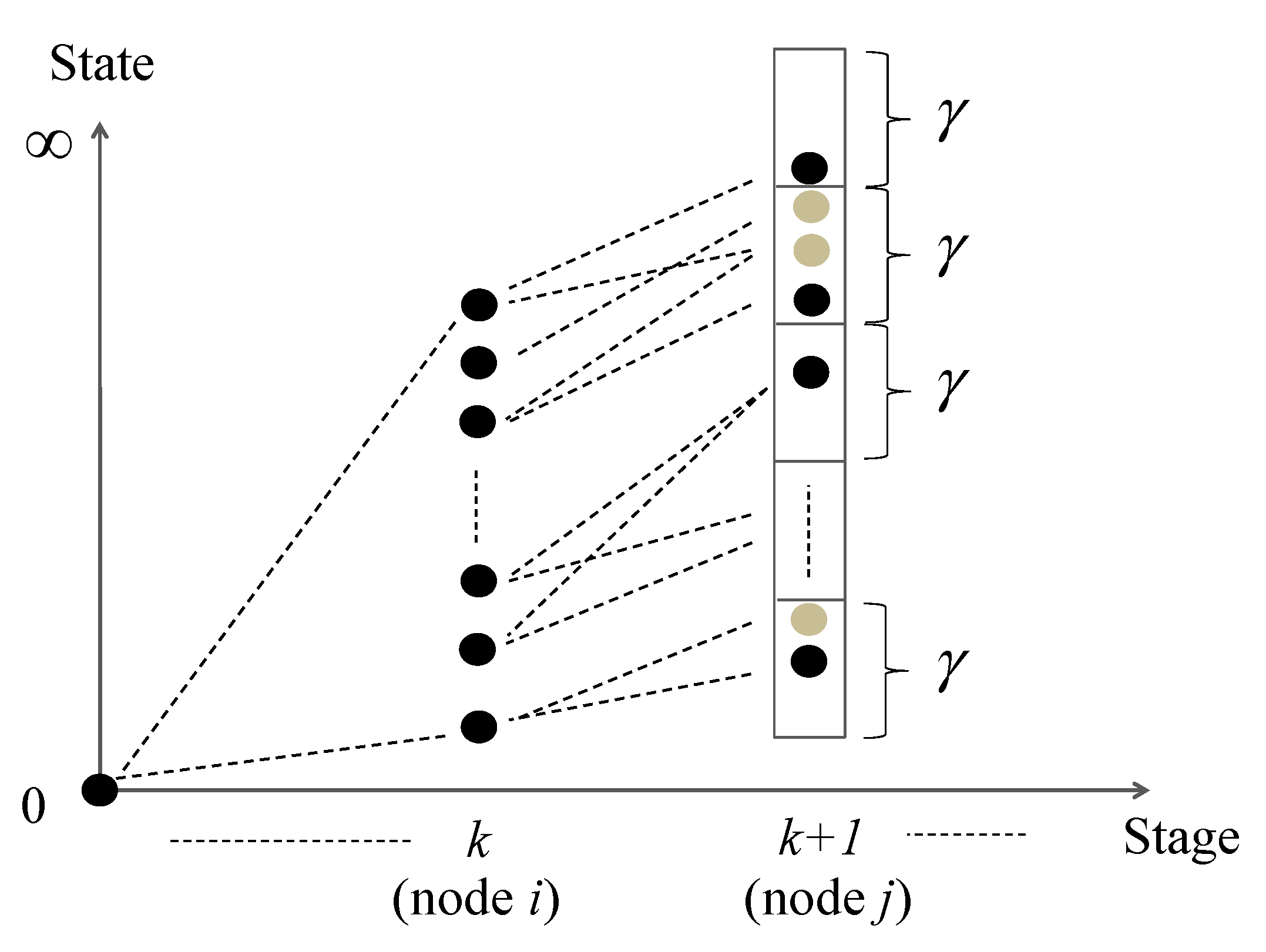
The proposed approach based on a dynamic programming has a backward recursion structure and requires explicit computation of total travel times from the origin to each node. The arrival time at each node can in theory be any continuous value spanning from zero to infinity. Thus, an adaptive discretization approach is used to partition the continuous state space into discrete grids. In this way, we can define a countable set of explicit states at all stages of the given problem before the backward recursive procedures are conducted.

Figure 1. Expansion and selection of the possible states.

Figure 1. Expansion and selection of the possible states.

Figure 1 describes how the states are selectively chosen in the next stage. In this figure, the x-axis represents stages, how many nodes have been explored in the given network including the current node, and y-axis represents the states, arrival times at each node. Note that node i and node j where (i,j) ∈ A are associated with the stage k and stage k + 1, respectively. We observe that as the stage proceeds from k (with node i) to k + 1 (with node j), the number of possible arrival times at the stage k + 1 rapidly increases. Thus, we discretize the state space into mutually disjointed uniform grids with a certain size γ and selectively consolidate all arrival times in each grid as one state (i.e., represented by black dots in Figure 1). The possible arrival times at a stage k + 2 (with node z) where (j,z) ∈ A can be obtained based on the selected arrival times (i.e., black dots) in the stage k + 1. The detailed procedures are described as follows:

Step 0.

Initialization. Let T_i = {0} if i = g; T_i = {}, otherwise. Set the candidate list S = {g}. Obtain in-degree of a node i, indeg(i), ∀i ∈ V \ {g}; indeg(i) = 0, otherwise.

Step 1.

Select node i from the set S, which is the first element in the set.

step 2.

For all nodes j where link (i,j) ∈ A exists, if indeg(j) > 0, conduct the following analysis:

Stemp 2a.

Calculate all possible states (i.e., arrival times) at node j based on the set T_i.

Stemp 2b.

Incorporate the result obtained in Step 2a into the current state set at node j, T_j, and selectively choose some elements among the total elements in T_j.

Stemp 2c.

If j ∉ S, include node j to the set S as the last element in the set.

Stemp 2d.

Update indeg(j) ← indeg(j) − 1.

Step 3.

Eliminate node i from the set S. If S = {} or indeg(i) = 0, ∀i ∈ V terminate the algorithm and set T_i contains selectively chosen states at node i, ∀i ∈ V; otherwise, go to Step 1.

4.2. Deterministic Shortest Path Heuristic

In many real roadway networks, truck drivers need to select the next travel link in real time (e.g., within several seconds). Thus, this section proposes a heuristic to find not only a feasible solution in a very short computation time even for very large networks but also an upper bound for the optimum solution. In this algorithm, the shortest path from the origin to the destination is obtained using the expected link cost which includes only link travel time and related emissions as cost components. Once the truck reaches the destination, penalties based on the arrival time at the destination are incorporated to generate the expected total cost. The detailed algorithm is described as follows:

Step 0.

Initialization. Set λ_i = 1, ∀i ∈ V \ {g} to represent candidate nodes, which have been scanned; λ_i = 0, otherwise to represent a current node. Set the total travel time to a node i, τ_i = ∞, ∀i ∈ V \ {g}; τ_i = 0, otherwise. Set the expected total cost to reach a node i, μ_i = ∞, ∀i ∈ V \ {g}; μ_i = 0, otherwise. Set an index I =0.

Step 1.

For each node i′ ∈ V where λ_i = 0, conduct the following analysis for each link (i′,j) ∈ A:

Step 1a.

Calculate expected cost for traveling link (i′,j), π_(i′,j), as follows:

• If node j ≠ s, ${\pi }_{(i^{\prime },j)}={\mathrm{\int }}_0^{+\infty }{f}_{U_{i^{\prime }j}}\left(u_{i^{\prime }j}\right)\cdot \left\{\mathrm{\alpha }\frac{d_{i^{\prime }j}}{u_{i^{\prime }j}}+\mathrm{\beta }W\left(u_{i^{\prime }j}\right)\right\}d{u}_{i^{\prime }j}$ ;
• otherwise, ${\mathrm{\pi }}_{(i^{\prime },j)}={\mathrm{\int }}_0^{+\infty }{f}_{U_{i^{\prime }j}}\left(u_{i^{\prime }j}\right)\cdot \left\{\mathrm{\alpha }\frac{d_{i^{\prime }j}}{u_{i^{\prime }j}}+\mathrm{\beta }W\left(u_{i^{\prime }j}\right)+P\left({\mathrm{\tau }}_{i^{\prime }}+\frac{d_{i^{\prime }j}}{u_{i^{\prime }j}}\right)\right\}d{u}_{i^{\prime }j}$.

Step 1b.

If ${\mathrm{\mu }}_j>{\mathrm{\mu }}_{i^{\prime }}+{\mathrm{\pi }}_{(i^{\prime },j)}$ , update ${\mathrm{\mu }}_j\leftarrow {\mathrm{\mu }}_{i^{\prime }}+{\mathrm{\pi }}_{(i^{\prime },j)}$, ${\mathrm{\tau }}_j\leftarrow {\mathrm{\tau }}_{i^{\prime }}+{\mathrm{\int }}_0^{+\infty }{f}_{U_{i^{\prime }j}}\left(u_{i^{\prime }j}\right)\cdot \left(\frac{d_{i^{\prime }j}}{u_{i^{\prime }j}}\right)d{u}_{i^{\prime }j}$, and $I\leftarrow I+1$, and let ${\mathrm{\lambda }}_j=2$.

Step 2.

For all nodes i ∈ V, if there are nodes with λ_i = 0, let λ_i = 1; if there are nodes with λ_i = 2, let λ_i = 0.

Step 3.

If I ≠ 0, let I = 0 and go to Step 1; otherwise, terminate the algorithm and μ_s represents the expected total cost.

5. Case Studies

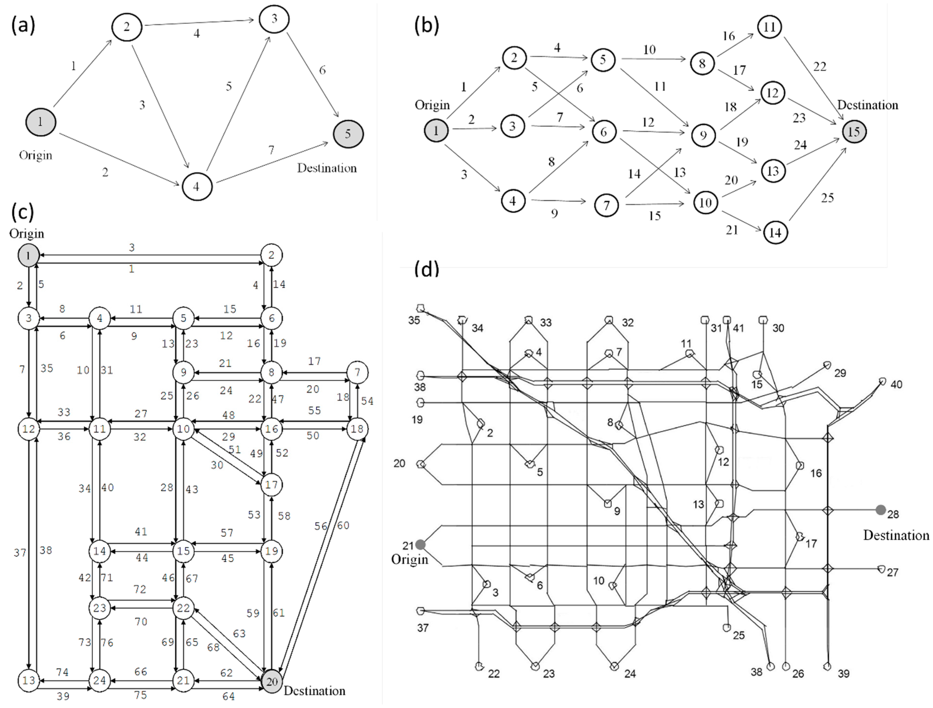
The proposed model and solution algorithms are coded on a personal computer with a 3.4 GHz CPU and 8 GB memory. Numerical experiments are first conducted on two simple and small imaginary networks: a 5-node and 7-link test network [44] as shown in Figure 2a and a 15-node and 25-link test network [30] as shown in Figure 2b. The emphasis with these small networks is to investigate the performance of the proposed solution algorithms. Then, the proposed approach is applied to more complex U.S. urban transportation networks [45]: a 24-node and 76-link Sioux Falls network, as shown in Figure 2c, and a 416-node and 914-link Anaheim network, as shown in Figure 2d.

Figure 2. (a) 5-node and 7-link network [44]; (b) 15-node and 25-link network [30]; (c) 24-node and 76-link Sioux Falls network [45]; (d) 416-node and 914-link Anaheim network [45].

Figure 2. (a) 5-node and 7-link network [44]; (b) 15-node and 25-link network [30]; (c) 24-node and 76-link Sioux Falls network [45]; (d) 416-node and 914-link Anaheim network [45].

In Figure 2a–c, the numbers in circles represent node indices and those near links denote link indices. Due to the complexity of the network, Figure 2d only shows selected node indices. Origin-destination pairs with relatively long shipment distances are randomly selected and represented by grey circles. Recall that t is the total travel time and h is the scheduled travel time (hours). We assume that the penalty cost function P (⋅) is piece-wise linear, as follows:

$$P\left(t\right)=\{\begin{array}{c}100(t-h), \text{if} t\ge h,\\ -10(t-h), \text{otherwise}.\end{array}$$

(4)

Let W₁(U_ij), W₂(U_ij), sustainability-83734, and W₄(U_ij) be the freight truck emission rate functions (grams/veh-mile) for CO₂, VOC, NO_X, and PM respectively on a link (i,j) ∈ A [43]. Thus, the combined truck emission model in Equation (1) can be represented as follows:

$$\begin{array}{l}\mathrm{\beta }W\left(U_{ij}\right)={\mathrm{\beta }}_1{W}_1\left(U_{ij}\right)+{\mathrm{\beta }}_2{W}_2\left(U_{ij}\right)+{\mathrm{\beta }}_3{W}_3\left(U_{ij}\right)+{\mathrm{\beta }}_4{W}_4\left(U_{ij}\right)\\ =k_1+k_2{U}_{ij}+\frac{k_3}{U_{ij}}+\frac{k_4}{{U_{ij}}^2}+\frac{k_5}{{U_{ij}}^3}\end{array}$$

(5)

where β₁ = 280 ($/tonCO₂), β₂ = 200 ($/tonVOC), β₃ = 200 ($/tonNO_X), and β₄ = 300 ($/tonPM₁₀) are parameters that convert the weight of the corresponding emissions into the monetary values [46,47]. This gives the total emission cost when the truck travels on link (i,j). Note that the unit price of PM10 is used to estimate the total PM emission cost (due to lack of data). Coefficients in the combined emission cost Function (5) are k₁ = 0.7121, k₂ = −0.0128, k₃ = 0.0848, k₄ = 6.2065, and k₅ = 2.1979 × 10⁻⁶. The function hence has a parabolic shape which is minimized when the truck speed is around 44 mph. Also, in Equation (1) we choose α = 20 ($/hr) [48].

The probability density function of the truck speed on each link is assumed to follow a randomly generated log-normal distribution, whose mean and standard deviation are uniformly and independently drawn from (20,60) mph and (10,15) mph, respectively. States at each stage are defined based on the states at the previous stage, using five representative vehicle speeds including minimum (truck speed at the 0.1th percentile), maximum (truck speed at the 99.9th percentile), mean speed, average between the minimum and mean speed, and average between the maximum and mean speed. For each test network, initial grid size (γ < 1) is arbitrarily selected and decreased with a small step size (0.005) until convergence.

Table 1 summarizes computational results. Column (b) specifies the two different algorithms applied in each test example. For the dynamic programming approach, the grid size (γ) at which the objective cost converged is also included. Column (c) represents the minimum expected total costs associated with different algorithms and column (d) shows the percentage differences between the heuristic solutions and the dynamic programming approach solutions. Column (e) shows the computation times.

Column (c) of Table 1 shows that the minimum expected total cost obtained from the dynamic programming approach is always lower than that from the deterministic shortest path heuristic. The percentage difference in column (d) gradually increases with the network size; the difference is notable in the largest network tested (i.e., the Anaheim network example). Column (e) shows that the solution times of the deterministic shortest path heuristic are much shorter than those of the dynamic programming approach.

Table 1. Computational results of the numerical examples.

(a) Network	(b) Algorithm	(c) Min. expected total cost ($)	(d) = (Heuristic – DP)/DP (%)	(e) Solution time (sec)
5-node and 7-link network	Shortest path heuristic	33.33	2.54	0.008
	Dynamic programming (γ = 0.025)	32.51	-	0.218
15-node and 25-link network	Shortest path heuristic	20.49	2.61	0.009
	Dynamic programming (γ = 0.030)	19.97		0.725
24-node and 76-link Sioux Falls network	Shortest path heuristic	49.55	2.82	0.011
	Dynamic programming (γ = 0.050)	48.19	-	160.052
416-node and 914-link Anaheim network	Shortest path heuristic	132.60	21.02	0.071
	Dynamic programming (γ = 0.040)	109.57	-	8741.145

Table 1. Computational results of the numerical examples.

(a) Network	(b) Algorithm	(c) Min. expected total cost ($)	(d) = (Heuristic – DP)/DP (%)	(e) Solution time (sec)
5-node and 7-link network	Shortest path heuristic	33.33	2.54	0.008
	Dynamic programming (γ = 0.025)	32.51	-	0.218
15-node and 25-link network	Shortest path heuristic	20.49	2.61	0.009
	Dynamic programming (γ = 0.030)	19.97		0.725
24-node and 76-link Sioux Falls network	Shortest path heuristic	49.55	2.82	0.011
	Dynamic programming (γ = 0.050)	48.19	-	160.052
416-node and 914-link Anaheim network	Shortest path heuristic	132.60	21.02	0.071
	Dynamic programming (γ = 0.040)	109.57	-	8741.145

To investigate how emission cost consideration will affect the truck driver’s route decision and eventually influence the expected total cost, two scenarios are designed as follows: (i) a conventional approach in which the emission cost is ignored in the truck driver’s routing decision process (but we do include the emission cost into total cost evaluation based on the truck driver’s routing decision), and (ii) the proposed dynamic programming approach in which the emission cost is incorporated into the truck driver’s route decision process. Columns (c)–(f) of Table 2 show the minimum expected total cost and the monetary values of its itemized components, i.e., the minimum expected total cost in column (c) is the same as sum of total travel time cost in column (d), emission cost in column (e), and penalty cost in column (f). Note that the cost differences between two scenarios in columns (c)–(f) are presented in every third and fourth rows of each network example.

Compared to the solutions from the conventional approach, the proposed dynamic programming approach results in a smaller minimum expected total cost for all study examples, as shown in column (c) of Table 2. In the first, second, and last examples, decrease in the total cost has been mainly due to a large reduction in the emission cost. The third example shows a different case in which the proposed approach has caused a large cost reduction in the total travel time, which is offset by significant cost increase in the penalty; the total cost saving has been mainly from the reduced emission cost.

Table 2. Comparisons between two different scenarios.

(a) Network	(b) Scenario	(c) Min. expected total cost ($)	(d) Travel time ($)	(e) Emissions ($)	(f) Penalty ($)
5-node and 7-link network	Conventional approach *	35.45	13.88	13.76	7.80
	Proposed approach **	32.51	14.39	10.81	7.30
	Cost difference ***	2.94	−0.51	2.95	0.50
		8.29%	−3.67%	21.42%	6.41%
15-node and 25-link network	Conventional approach	21.22	6.35	5.90	8.96
	Proposed approach	19.97	6.73	4.46	8.78
	Cost difference	1.25	−0.38	1.44	0.19
		5.87%	−5.97%	24.38%	2.08%
24-node and 76-link Sioux Falls network	Conventional approach	52.75	24.57	15.57	12.61
	Proposed approach	48.19	14.52	9.22	24.45
	Cost difference	4.56	10.05	6.36	−11.84
		8.64%	40.90%	40.82%	−93.93%
416-node and 914-link Anaheim network	Conventional approach	114.38	67.00	47.00	0.39
	Proposed approach	109.57	67.29	41.81	0.47
	Cost difference	4.81	−0.29	5.19	−0.08
		4.21%	−0.44%	11.04%	−21.76%

^* Conventional approach: Ignoring emission cost in the truck driver’s routing decision process; ^** Proposed approach: Considering emission cost in the truck driver’s routing decision process; ^*** Cost difference = Cost from the conventional approach − Cost from the proposed approach.

Table 2. Comparisons between two different scenarios.

(a) Network	(b) Scenario	(c) Min. expected total cost ($)	(d) Travel time ($)	(e) Emissions ($)	(f) Penalty ($)
5-node and 7-link network	Conventional approach *	35.45	13.88	13.76	7.80
	Proposed approach **	32.51	14.39	10.81	7.30
	Cost difference ***	2.94	−0.51	2.95	0.50
		8.29%	−3.67%	21.42%	6.41%
15-node and 25-link network	Conventional approach	21.22	6.35	5.90	8.96
	Proposed approach	19.97	6.73	4.46	8.78
	Cost difference	1.25	−0.38	1.44	0.19
		5.87%	−5.97%	24.38%	2.08%
24-node and 76-link Sioux Falls network	Conventional approach	52.75	24.57	15.57	12.61
	Proposed approach	48.19	14.52	9.22	24.45
	Cost difference	4.56	10.05	6.36	−11.84
		8.64%	40.90%	40.82%	−93.93%
416-node and 914-link Anaheim network	Conventional approach	114.38	67.00	47.00	0.39
	Proposed approach	109.57	67.29	41.81	0.47
	Cost difference	4.81	−0.29	5.19	−0.08
		4.21%	−0.44%	11.04%	−21.76%

^* Conventional approach: Ignoring emission cost in the truck driver’s routing decision process; ^** Proposed approach: Considering emission cost in the truck driver’s routing decision process; ^*** Cost difference = Cost from the conventional approach − Cost from the proposed approach.

Results show that savings from the proposed modeling approach are larger in the last two large-scale urban network examples, in which each truck can save more than $4.5 in terms of total cost and $5.0 in terms of emission cost for the given route of travel. Note that this cost saving is for one individual truck and one origin-destination pair delivery. If the proposed environmental-friendly routing policy can be implemented for all freight trucks operated in the study areas, a large reduction in adverse social cost can be expected. For example, annual vehicle miles traveled by freight trucks was estimated as 5,186,467 and average trip length for one freight truck was obtained as 74.5 miles per day in the city of Los Angeles [49]. From simple computation, the total number of freight truck trips in Los Angeles can be estimated as around 70,000 in one year. Therefore, around $313,000 for the total cost and $348,000 for the emission cost could be saved per year. This will improve urban air quality and contribute to enhanced public social welfare.

6. Conclusions and Future Study

We focus on urban transportation networks in which traffic congestion on each link, represented by the prevailing speed, follows a known independent probability distribution. A truck driver needs to decide the next traveling link at each network node so as to minimize the expected total cost which includes total delivery time, emissions, and a penalty for late or early arrival. This problem is formulated into a mathematical model, and two solution algorithms including a dynamic programming approach and a deterministic shortest path heuristic are provided. Suggested algorithms are tested on both small, imaginary networks and complex, large-scale urban transportation networks. Although solutions from the dynamic programming approach are always lower than those from the deterministic shortest path heuristic, the latter requires much shorter solution times. The results from the proposed approach are compared with those from the conventional approach (in which emission cost is ignored in truck driver’s routing decision process) to investigate the trade-off among different cost components. It was shown that the minimum expected total cost can be reduced by applying the proposed methodology mainly due to a large reduction in the emission cost. The suggested methodology can be directly implemented into vehicle navigator system and the estimated annual savings are provided for the city of Los Angeles. This study can provide a scientific basis for policy makers to evaluate the impact of freight truck operations in urban areas on air quality, and to develop strategies to mitigate the negative environmental consequences especially under roadway congestion and various delivery constraints.

Future studies could consider limiting the number of uniform grids at each stage to a fixed number of partitions in the dynamic programming approach. This method will help reduce computational effort in large network examples. Second, time-dependent stochastic congestion state on each link can be applied to the current problem. Then, the link travel time and the emissions will be affected by stochastic truck speed on the link as well as truck arrival time at the link starting node. Third, we can include local and collector roads to represent urban transportation networks, where truck speed on downstream links will be correlated to that on upstream links. Lastly, the environmental impacts from the transportation activities can be further applied to other stochastic network optimization problems such as stochastic traveling salesman problems and stochastic vehicle routing problems.