Grain-Size Analysis of Debris Flow Alluvial Fans in Panxi Area along Jinsha River, China

Abstract

The basic geometric parameters of 236 debris flow catchments were determined by interpreting SPOT5 remote sensing images with a resolution of 2.5 m in a 209 km section along the Jinsha River in the Panxi area, China. A total of 27 large-scale debris flow catchments were selected for detailed in situ investigation. Samples were taken from two profiles in the deposition zone for each debris flow catchment. The φ value gradation method of the grain size was used to obtain 54 histograms with abscissa in a logarithmic scale. Five types of debris flows were summarized from the outline of the histogram. Four grain size parameters were calculated: mean grain size, standard deviation, coefficient of skewness, and coefficient of kurtosis. These four values were used to evaluate the features of the histogram. The grain index that reflects the transport (kinetic) energy information of debris flows was defined to describe the characteristics of the debris-flow materials. Furthermore, a normalized grain index based on the catchment area was proposed to allow evaluation of the debris flow mobility. The characteristics of the debris-flow materials were well-described by the histogram of grain-size distribution and the normalized grain index.

1. Introduction

The Wenchuan Earthquake triggered more than 15,000 landslides and rock collapses [1]. After a few months, a rainstorm on 24 September 2008 triggered a large number of debris flows in the region. A detailed field investigation and desk-based analysis was conducted by Tang et al. [2]. In addition, a second earthquake of magnitude 6.1 occurred on 30 August 2008, 500 km south of the epicenter of the Wenchuan Earthquake, located on the border of Sichuan and Yunnan provinces near the city of Panzhihua along the Jinsha River. The earthquakes generated large amounts of loose materials, which easily led to debris-flow disasters [3,4,5,6,7]. The area (Panxi area) for the present study is located near the abovementioned earthquake epicenters in the transitional zone between the Qinhai-Tibet and Yun-Gui Plateaus. This area is characterized by mountains and deep valleys, with poor vegetation cover, and a very high frequency of debris flows.

Damage caused by debris flows occurs during the transportation of material and in deposition zones. Debris flow material with greater transport energy has greater destructive power. If a debris flow has a larger mean particle diameter, more coarse grains are contained in a debris flow, and the flow has higher kinetic energy. Therefore, material parametric studies have attracted the attention of researchers [8,9,10,11]. Many scholars try to establish correlations between the debris flow activity and certain parameters, such as shear strength, density, porosity, and a plasticity index related to the loose materials [12,13,14,15]. According to Sumner et al. [16] and Scotto di Santolo et al. [17], who mixed different sized grains to generate gravity flows, grain size determines the characteristics of the debris-flow materials. The size of the largest transported boulders provided by deposits (such as screes) in the basin can be used to estimate the kinetic energy of debris flows. Bardou et al. [18] indicated that large changes occurred in grain-size distribution from source materials to the deposits in the alluvial fan. The grain-size distribution can reflect the characteristics of the debris flow transport, including the transport energy. Kokusho and Hiraga [19] and Federico and Cesali [20] stated that the dissipated energy ratio increased with increasing fines content and decreasing mean grain size. Wang et al. [21] interpreted the relationship between debris flow material and the grain size distribution by stating that the grain size affected the propensity of material to be mobilized during rainfall events. The fines content influences the behavior of the water/solid mixture and the depositional style of debris flows. Wang [22] and Zhang et al. [23] indicated that the kinetic energy and the head height of a debris flow surge increased with an increase of transported materials. Current research places emphasis on the grain-size distribution of debris-flow materials. Five types of debris flows were proposed, reflecting different transport energies of the debris flows. In addition, this study proposed two parameters, which are based on the grain size distribution and the catchment area, to quantitatively describe these types of debris flows.

2. Study Region

The study region is located on the southeastern boundary of the Qinhai-Tibet Plateau. High mountains and deep gorges occur in this area and make the geomorphological and topographical scenes around the study area varied (Figure 1a).

Foehn winds occur in the study area. The Hengduan Mountains are located between the Tibet Autonomous Region and Sichuan/Yunnan Provinces and strike north–south with an elevation from 4000 m to 5000 m. The southwesterly warm moist current from the Bay of Bengal in the Indian Ocean during summer is obstructed by the Hengduan Mountains, forming a Foehn wind. During winter, the dry continental current from Iran arrives in this region. Therefore, this area receives relatively little annual rainfall.

The borders and drainage system of the study region were determined by the location of a proposed reservoir in the lower reaches of the Jinsha River (Figure 1b). The right and left banks of Wudongde Dam are in Yunnan and Sichuan provinces, respectively. Debris flow catchments are mainly developed along the banks of the Jinsha River. The route of the Jinsha River is tortuous, resembling the letter V. While Wudongde Dam and Panzhihua City lie 95 km apart, the river channel flows for 209 km.

Figure 1. (a) Google images indicating the location of the study region; (b) Digital elevation model images.

Figure 1. (a) Google images indicating the location of the study region; (b) Digital elevation model images.

The Jinsha River has five large-scale tributaries in the study region. The Yalongjiang, Chenhe, and Canyuhe rivers flow in from the left bank of Jinsha River, and the Longchuanjiang and Menguohe rivers flow in from the right bank.

The loose materials in the study region are characterized by Longjie fine sand layers, Madianhe layers, red-bed layers, and completely weathered metamorphic rocks. The Longjie fine sand layers are composed of fine unconsolidated grains and are believed to have formed in standing water (Figure 2a). The Madianhe materials are composed of silts and gravels (Figure 2b). A mass of secondary cracks has developed in the Longjie fine sand and Madianhe layers. The calcareous structures in these two layers are easily destroyed on contact with water because the cementitious material between individual grains dissolves either partially or completely. Therefore, the Longjiefine sand and Madianhe layers collapse easily. The red-bed layers are composed of completely weathered sandstone and mudstone rocks as well as shales, all from the Jurassic to Triassic periods (Figure 2c). The completely weathered metamorphic rocks are mainly composed of slate, schist, and phyllite (Figure 2d). The grains in the red-bed layers and completely weathered metamorphic rocks are not compact. Therefore, these two types of loose materials easily collapse. In addition to the aforementioned loose materials, other kinds of loose materials, such as collapse deposits and ancient landslides, are also distributed in the debris flow catchments.

Figure 2. Main loose materials developed in the study region: (a) Longjie fine sand layer; (b) Madianhe layer; (c) Red-bed layer; and (d) Metamorphic layer (phyllite).

Figure 2. Main loose materials developed in the study region: (a) Longjie fine sand layer; (b) Madianhe layer; (c) Red-bed layer; and (d) Metamorphic layer (phyllite).

3. Features of the Debris Flows

The 236 debris flow catchments can be detected by interpreting the SPOT5 remote sensing images in the study region along the Jinsha River [24,25].Only large-scale debris flows affect the stability of the dam site. Therefore, 27 large-scale debris flow catchments were investigated (Table 1). Yanshuijin, which is one of the 27 debris flow catchments, was selected for a detailed description provided in this paper.

The Yanshuijin debris flow catchment is located on the left bank of the Jinsha River. The Longchuanjiang River, a tributary to the Jinsha River, is located on the opposite bank. The Yanshuijin debris flow catchment has the following main features, obtained from the interpretation of SPOT5 remote sensing images (Figure 3).The catchment area covers 45.58 km², with a main channel 14,430 m long. The largest elevation difference from the initiation zone to the deposition zone is 1.35 km. The average gradient of the main channel is 22.6°. The spatial gully density of the catchment is 9.25 km/km². The curvature of the main valley is 1.22. The potential reserve of loose materials is 925×10⁴ m³. The maximum width and diameter of the accumulation fan are 960 and 460m, respectively. The Jinsha River is generally from 110 m to 210 m wide in the area of the accumulation fan.

Table 1. The basic information ofthe 27 large-scale debris flow catchments.

Debris Flow Catchment	Xiabaitan	Shangbaitan	Zhugongdi	Yindigou	Canyuhe	Xiushuihe	Menggu	Jiachehe	Hujia
Catchement area (km2)	3.1	0.9	6.5	60.5	256.0	8.6	37.1	15.6	8.6
Maximum elevation difference (km)	3.08	1.87	4.98	20.17	29.63	2.20	10.52	5.07	5.16
Melton’s ruggedness number	0.99	2.05	0.77	0.33	0.12	0.26	0.28	0.33	0.60
Debris Flow Catchment	Kuashan	Zhuzhahe	Heizhe	Yanshuijin	Nuozhacun	Mapidi	Zhangmuhe	Hepiao	Jiaoping
Catchement area (km2)	6.7	152.6	51.7	48.6	32.6	7.2	4.6	9.1	46.9
Maximum elevation difference (km)	5.09	26.30	13.90	14.43	10.50	2.62	5.39	6.83	12.90
Melton’s ruggedness number	0.76	0.17	0.27	0.30	0.32	0.36	1.17	0.75	0.28
Debris Flow Catchment	Tianfanghe	Zhiligou	Yajiede	Pingdicun	Mutudahe	Daqiangou	Mengguohe	Fapagou	Jiali
Catchement area (km2)	13.1	120.6	22.3	24.2	98.0	18.9	620.8	24.1	31.8
Maximum elevation difference (km)	5.60	15.80	9.30	9.90	20.20	5.10	28.70	13.12	7.32
Melton’s ruggedness number	0.43	0.13	0.42	0.41	0.21	0.27	0.05	0.54	0.23

Table 1. The basic information ofthe 27 large-scale debris flow catchments.

Debris Flow Catchment	Xiabaitan	Shangbaitan	Zhugongdi	Yindigou	Canyuhe	Xiushuihe	Menggu	Jiachehe	Hujia
Catchement area (km2)	3.1	0.9	6.5	60.5	256.0	8.6	37.1	15.6	8.6
Maximum elevation difference (km)	3.08	1.87	4.98	20.17	29.63	2.20	10.52	5.07	5.16
Melton’s ruggedness number	0.99	2.05	0.77	0.33	0.12	0.26	0.28	0.33	0.60
Debris Flow Catchment	Kuashan	Zhuzhahe	Heizhe	Yanshuijin	Nuozhacun	Mapidi	Zhangmuhe	Hepiao	Jiaoping
Catchement area (km2)	6.7	152.6	51.7	48.6	32.6	7.2	4.6	9.1	46.9
Maximum elevation difference (km)	5.09	26.30	13.90	14.43	10.50	2.62	5.39	6.83	12.90
Melton’s ruggedness number	0.76	0.17	0.27	0.30	0.32	0.36	1.17	0.75	0.28
Debris Flow Catchment	Tianfanghe	Zhiligou	Yajiede	Pingdicun	Mutudahe	Daqiangou	Mengguohe	Fapagou	Jiali
Catchement area (km2)	13.1	120.6	22.3	24.2	98.0	18.9	620.8	24.1	31.8
Maximum elevation difference (km)	5.60	15.80	9.30	9.90	20.20	5.10	28.70	13.12	7.32
Melton’s ruggedness number	0.43	0.13	0.42	0.41	0.21	0.27	0.05	0.54	0.23

Figure 3. SPOT5 Remote sensing images of the Yanshuijin catchment.

Figure 3. SPOT5 Remote sensing images of the Yanshuijin catchment.

3.1. Accumulation Fan

Yanshuijin village is located at the left side on the accumulation fan (Figure 4). Signs of debris flow activity (e.g., mud balls) were observed on the accumulation fan during the site investigation (Figure 5). The color of the accumulation fan varies; red, purple, gray, and black are thoroughly mixed because of the complex composition of the material. Sandstone, marble, gneiss, and breccias can be found. The granulometric composition is also complex and silty clay particles, cobbles, and boulders can be found. The debris grains are poorly sorted, and the sphericity is subangular to subrounded.

Figure 4. General view of the Yanshuijin accumulative fan.

Figure 4. General view of the Yanshuijin accumulative fan.

Figure 5. Mud ball on the accumulative fan.

Figure 5. Mud ball on the accumulative fan.

3.2. Transportation Zone

The Yanshuijin debris flow catchment has a very long (3.6 km) and wide (150 m) transportation zone with an average slope of approximately5°. On the left bank of the transportation zone, the lithology is mainly characterized by inter bedded purple sandstone and siltstone from the Jurassic to Tertiary periods that is known as the red bed. Three large-scale ravines with a hill slope of greater than 25° exist. On the right bank of the transportation zone, the lithology is characterized by gray metamorphic rocks in Proterozoic Era, including phyllite, schist, gneiss, and marble. Four large-scale ravines in the area have a hill slope of 40°–50°. Faults and folds are developed with poor slope stability. A phyllite rockslide was triggered by the Panzhihua Earthquake (Figure 6). The residents there saw the slide occur during the earthquake. The main transportation zone has a letter V shape (Figure 7).

Figure 6. A phyllite rockslide on the right bank.

Figure 6. A phyllite rockslide on the right bank.

Figure 7. U-shaped main transportation zone.

Figure 7. U-shaped main transportation zone.

3.3. Initiation Zone

The initiation zone has an average hill slope of 52° and is composed of two main subsidiary zones (Figure 3). The larger subsidiary zone has the same strike (NNE) as the transportation zone. The smaller subsidiary zone has a NNW strike. Debris materials are mainly provided by collapses and slides from the Madianhe layer. The Madianhe layer is characterized by vertical slopes with a material thickness exceeding 100 m, which gives rise to collapses and slope failures. Therefore, enough loose materials are present in the initiation zone for debris flow activity to occur.

4. Methodology

The solid-carrying capacity from the initiation to the deposition zones is influenced by various factors in which the grain-size distribution is a very important feature and is analyzed in this study.

4.1. Data Collection

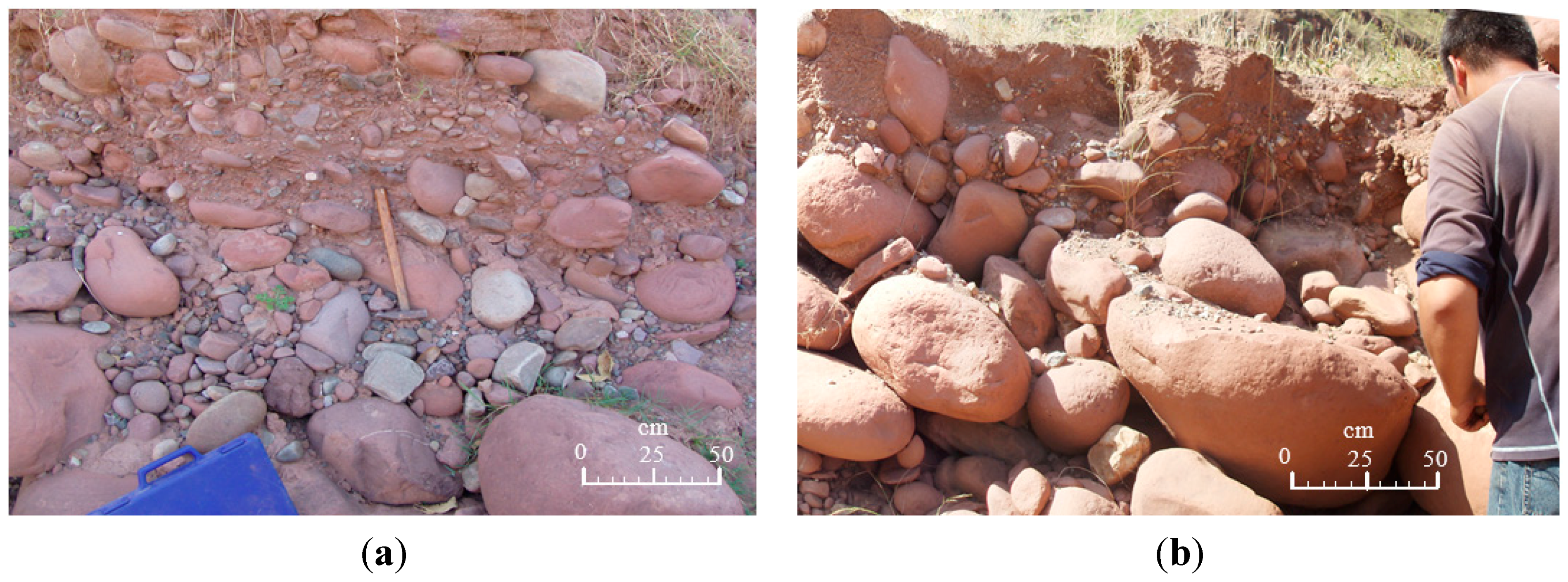
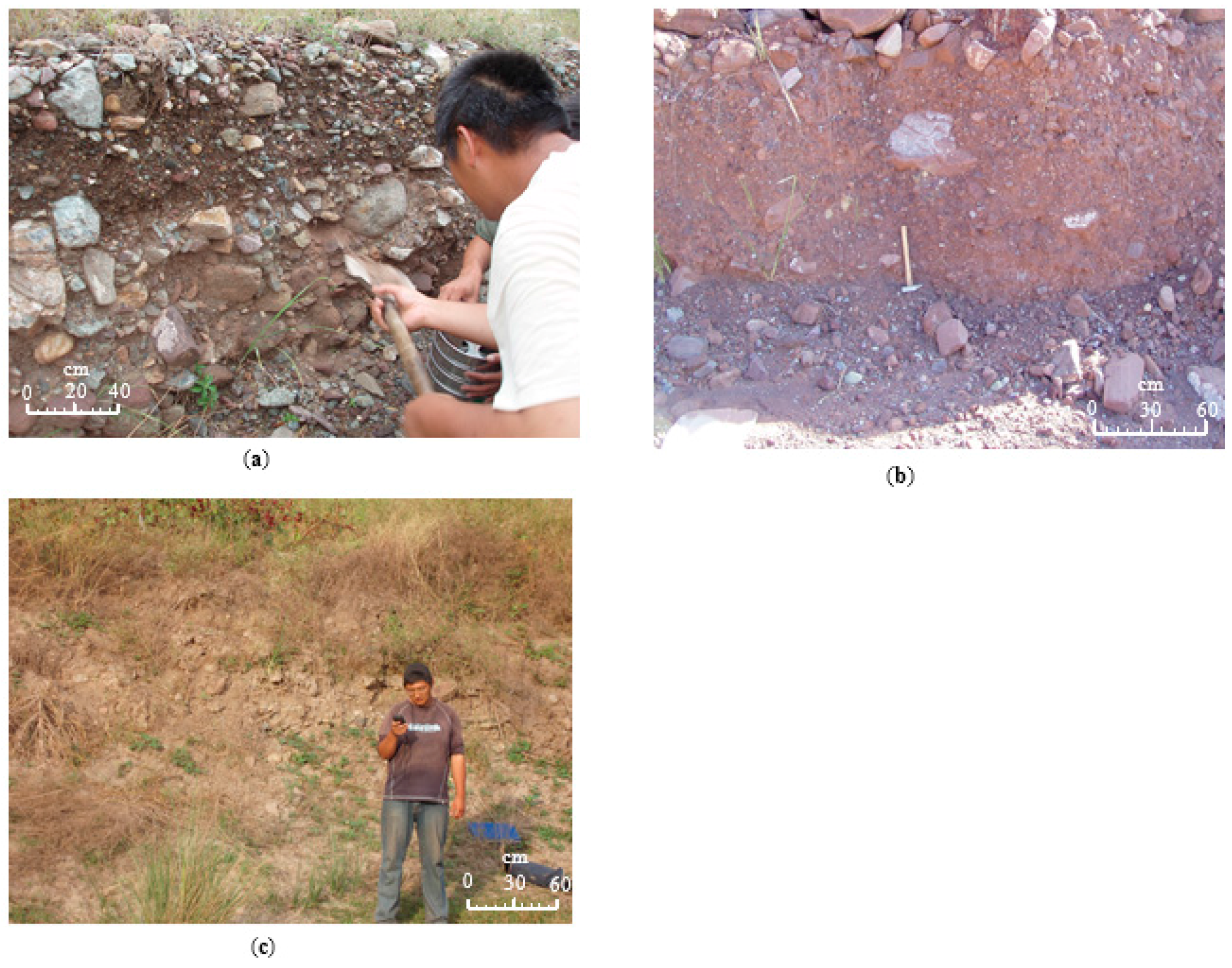
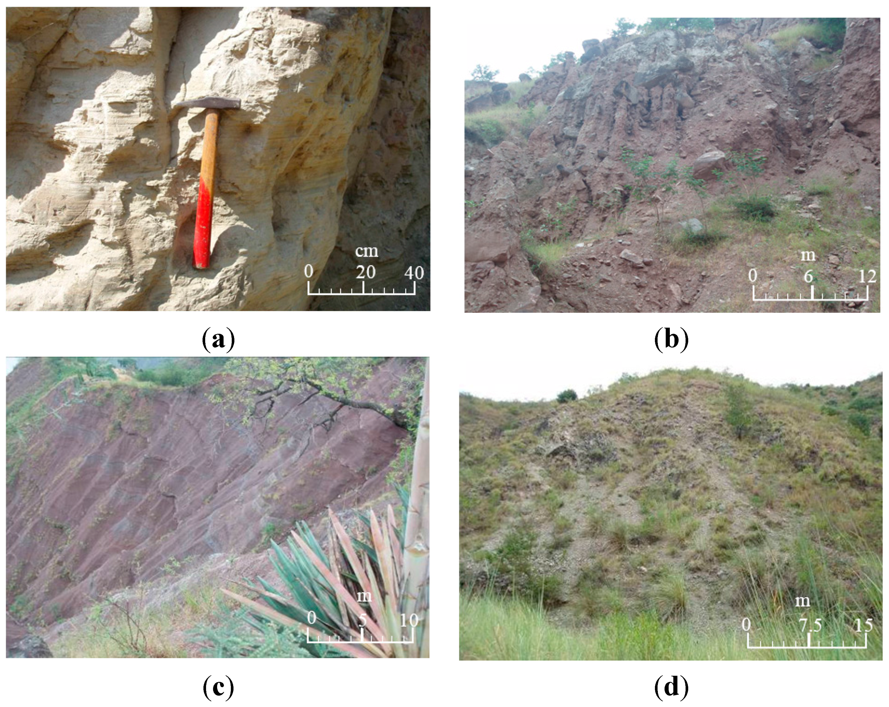
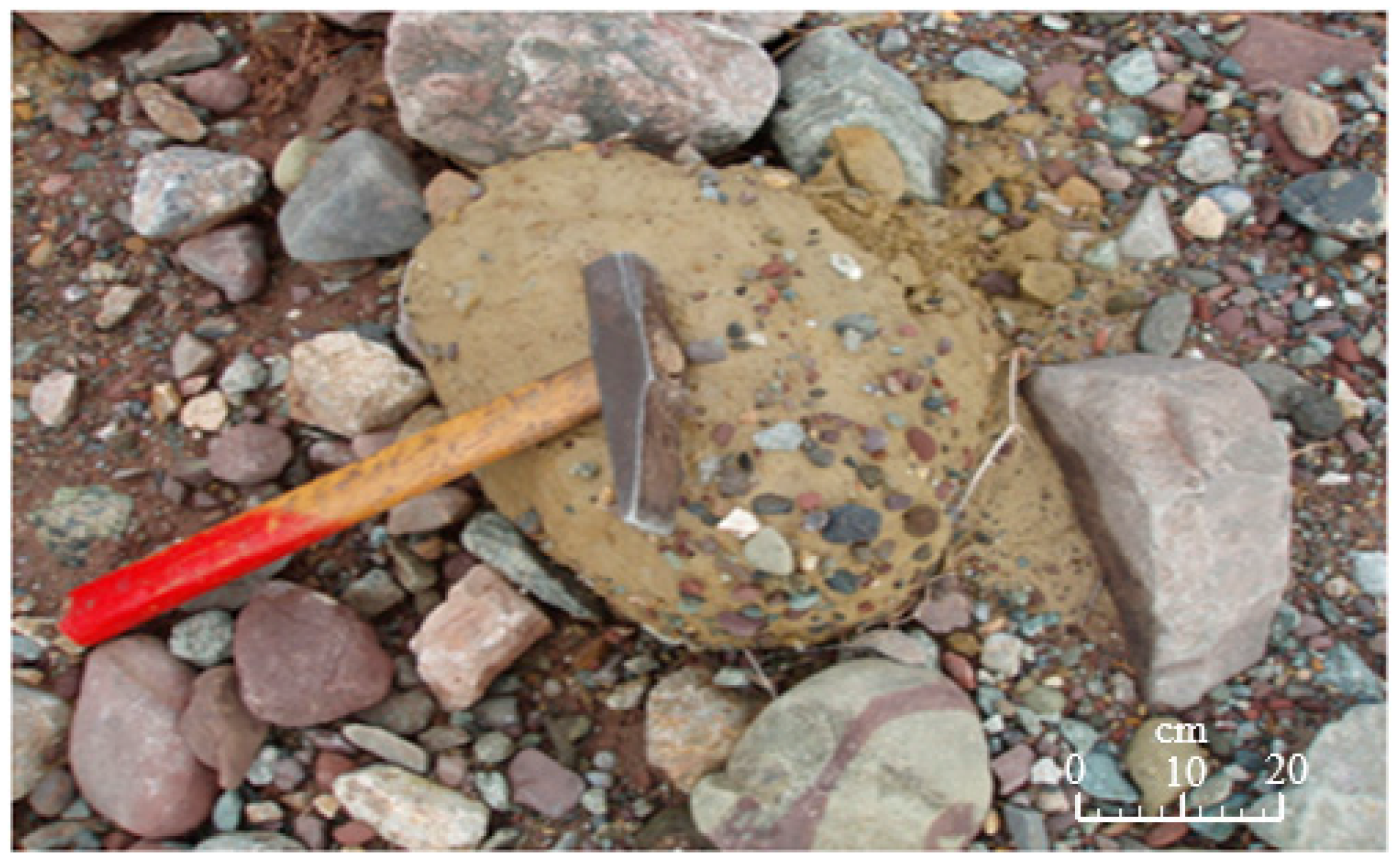
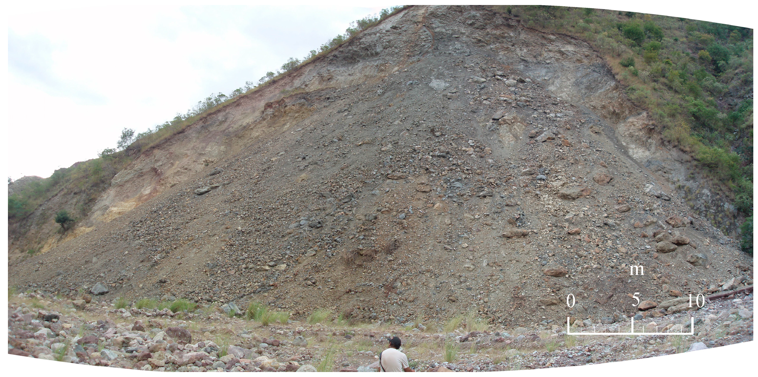
In situ sieve analysis provides a very convenient method for analyzing debris flows. Gully walls can be found on accumulation fans. Most of the gully walls are higher than 1 m; therefore, taking samples from the gully walls is relatively very easy. A set of sieves with sizes of 2, 5, 10, 20, 40, and 60 mm was used.

The smallest sieve size was 2 mm, meaning that particles smaller than 2 mm could not be quantified in situ. Under natural conditions, particles smaller than 2 mm could not be sufficiently dried easily, and some particles were in a pseudo-silty grain form. Samples with grain sizes smaller than 2 mm were taken to the laboratory, and further particle size analyses were performed using both small aperture sieves and the hydrometer method. Thus, the grain-size distribution curves with sizes of 0.075 mm to 60 mm were obtained.

Conducting size analysis for grains larger than 60 mm is impossible using only standard sampling and sieving procedures. Therefore, image analysis described by Tiranti et al. [26] was used to determine the size distribution of the large grains. Their study properly scaled and measured the images, and suitable scaled photos were taken of the sampling points. Consequently, the proportions of the grains larger than 60 mm visible in the images were estimated. Despite the problems inherent in reliably estimating the grain diameter (errors resulting from two-dimensional analysis), the image analysis provided a more feasible method than sieve analysis.

More than 10 kg of samples were required for the in situ test, and at least two repetitions of the tests were performed. Portable electronic scales with size of 230 × 230 mm and measuring range of 0.01 kg to 40 kg were used for weighting. Data obtained with the aforementioned methods were then compared and integrated.

4.2. Parametric Study

To describe the characteristics of the debris-flow materials, the modified φ value method [27] is recommended, applying Equation (1) to perform the grain-size conversion:

$$\text{ϕ}=-{\text{log}}_{2}d$$

(1)

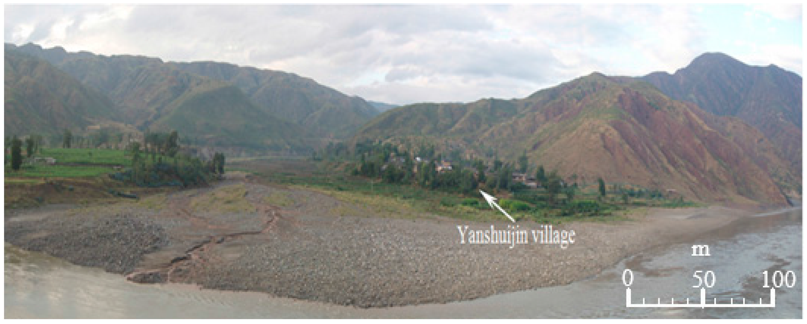
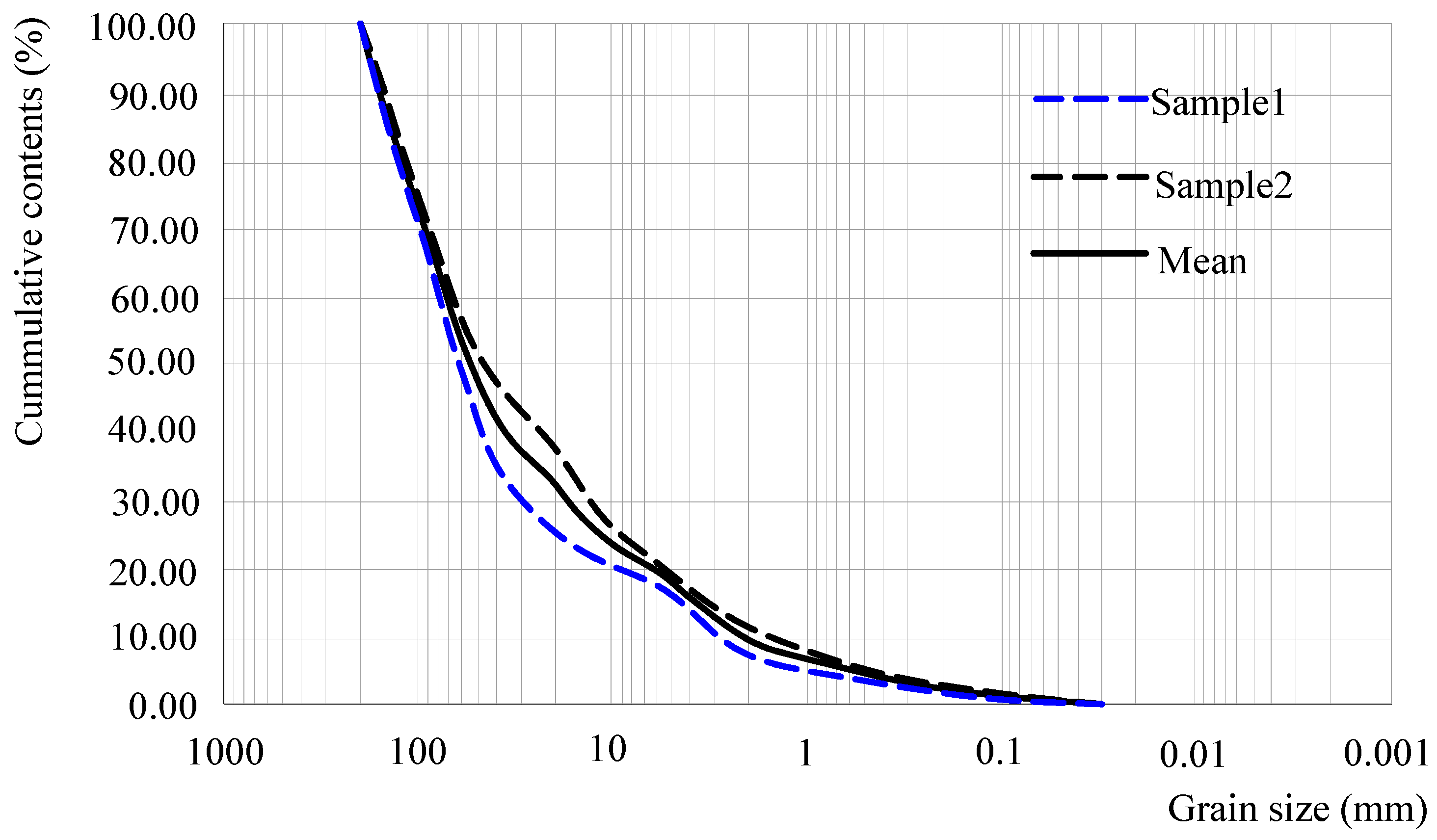
where d is the grain size (mm). Figure 8, which shows the grain size and the cumulative percentage content of the Yanshuijin deposition, was drawn in terms of Equation (1). The abscissa, which represents the grain size, has a logarithmic scale. Some of the significant indices can be obtained from Figure 8, such as φ₅, φ₁₆, φ₂₅, φ₅₀, φ₇₅, φ₈₄, and φ₉₅; the subscripts represent the cumulative percentage content. 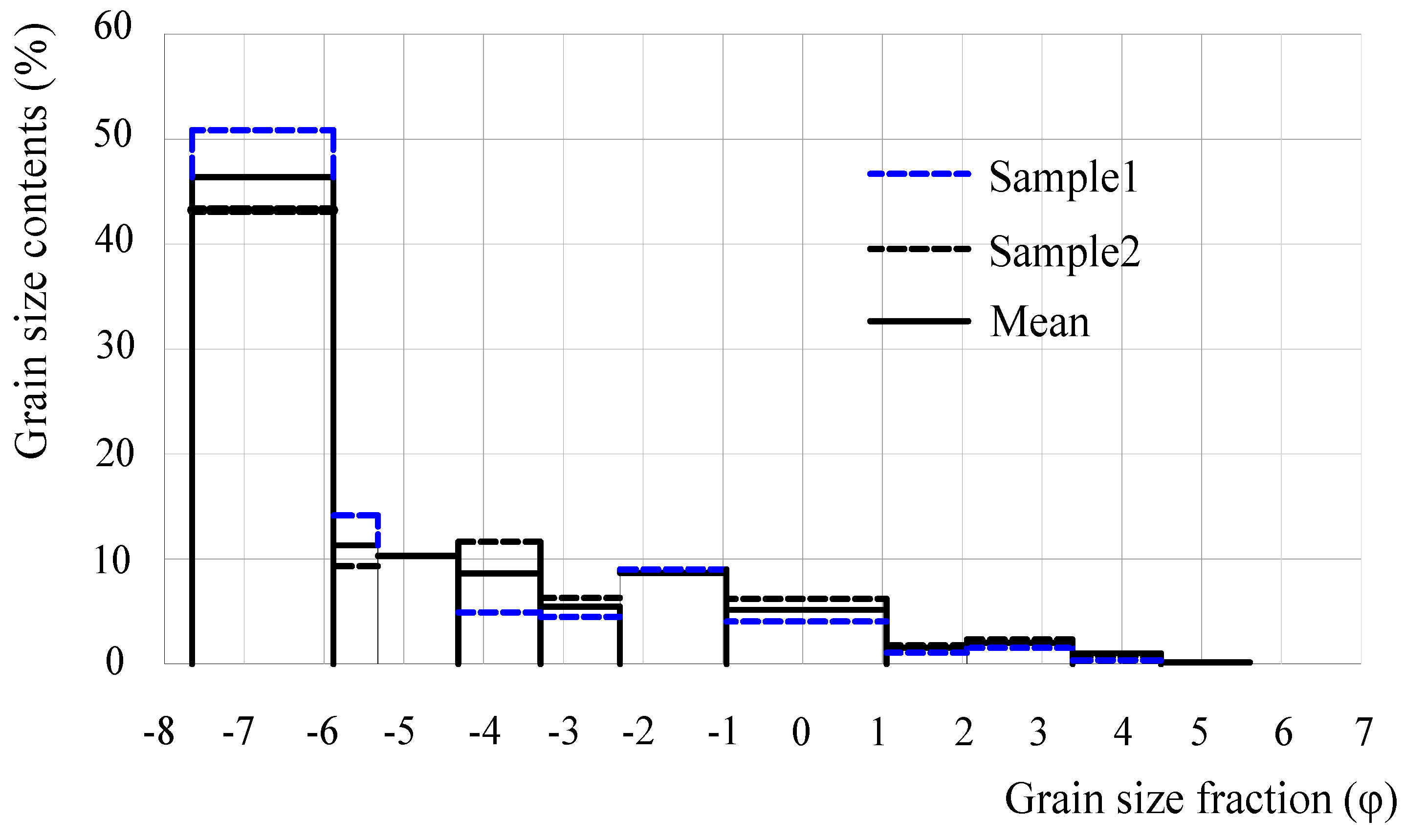Table 2 shows the corresponding values of d and φ. A histogram of the grain-size distribution relative to the φ value can be drawn (Figure 9).

Table 2. Corresponding values of d and φ.

d (mm)	0.005	0.01	0.05	0.1	0.25	0.5	2.0	5.0	10.0	20.0	40.0	60.0	200.0
φ	7.67	6.67	4.34	3.33	2.01	1.00	−1.0	−2.33	−3.33	−4.34	−5.34	−5.93	−7.67

Table 2. Corresponding values of d and φ.

d (mm)	0.005	0.01	0.05	0.1	0.25	0.5	2.0	5.0	10.0	20.0	40.0	60.0	200.0
φ	7.67	6.67	4.34	3.33	2.01	1.00	−1.0	−2.33	−3.33	−4.34	−5.34	−5.93	−7.67

Figure 8. Grain-size distribution of the Yanshuijin sediment.

Figure 8. Grain-size distribution of the Yanshuijin sediment.

Figure 9. Histogram of the grain-size distribution of the Yanshuijin deposition.

Figure 9. Histogram of the grain-size distribution of the Yanshuijin deposition.

To analyze the sedimentary transport environment and the characteristics of the debris-flow materials, the grain size parameter method suggested by Folk and Word [28] was used. The mean grain size M is expressed by Equation (2):

$$M=\frac{{\text{ϕ}}_{16}+{\text{ϕ}}_{50}+{\text{ϕ}}_{84}}{3}$$

(2)

When the grain sizes follow a normal distribution, the mean, median, and modal grain diameters reflect the distribution center and the kinetic energy of the sediment. The mean grain size and the mean gain diameter of the Yanshuijin deposition were equal to –5 and 30 mm, respectively.

The standard deviation shows the degree of variation from the mean. A low standard deviation indicates that the data points tend to be close to the mean, whereas high standard deviation indicates that the data are spread out over a large range of values. In this study, the standard deviation σ is expressed by Equation (3):

$$\text{σ}=\frac{{\text{ϕ}}_{84}-{\text{ϕ}}_{16}}{4}+\frac{{\text{ϕ}}_{95}-{\text{ϕ}}_5}{6.6}$$

(3)

The standard deviation, which expresses the degree of sorting of the deposition, is 2.60 in the Yanshuijin deposition (calculated by Equation (3)).The degree of sorting can be checked from Table 3, which is proposed by Folk and Word [28]. Table 3 shows the degree of sorting for the Yanshuijin deposition is very poor.

Table 3. Gradation standard of the degree of sorting according to σ.

Degree of Sorting	Extremely Good	Good	Fair	Medium	Poor	Very Poor	Extremely Poor
σ	<0.35	0.35–0.5	0.5–0.71	0.71–1	1–2	2–4	>4

Table 3. Gradation standard of the degree of sorting according to σ.

Degree of Sorting	Extremely Good	Good	Fair	Medium	Poor	Very Poor	Extremely Poor
σ	<0.35	0.35–0.5	0.5–0.71	0.71–1	1–2	2–4	>4

The coefficient of skewness is a measure of the degree of asymmetry in a distribution. In this study, the coefficient of skewness Sk is expressed by Equation (4):

$$SK=\frac{{\text{ϕ}}_{16}+{\text{ϕ}}_{84}-2{\text{ϕ}}_{50}}{2({\text{ϕ}}_{84}-{\text{ϕ}}_{16})}+\frac{{\text{ϕ}}_5+{\text{ϕ}}_{95}-2{\text{ϕ}}_{50}}{2({\text{ϕ}}_{95}-{\text{ϕ}}_5)}$$

(4)

The coefficient of skewness expresses the degree of symmetry of fine particles and coarse grains in the distribution curve relative to the location of the modal value. The sample from Yanshuijin contains mainly coarse grains; thus, the location of the modal value is skewed to the coarse-grain side (i.e., positively skewed). Most river sedimentation and turbidite fan materials belong from the range of positive to extremely positive skewness. The coefficient of skewness of the Yanshuijin deposition was 0.53, as calculated by Equation (4).The skewness gradation (Table 4) was recommended by Folk and Word [28]. The gradation of the Yanshuijin deposition materials is extremely positively skewed.

Table 4. Skewness gradation of the sedimentation.

Skewness	Extremely Negative	Negative	Symmetrical	Positive	Extremely Positive
SK	[−1.00, −0.3)	[−0.3, −0.1)	[−0.1, +0.1)	[+0.1, +0.3)	[+0.3, +1.0)

Table 4. Skewness gradation of the sedimentation.

Skewness	Extremely Negative	Negative	Symmetrical	Positive	Extremely Positive
SK	[−1.00, −0.3)	[−0.3, −0.1)	[−0.1, +0.1)	[+0.1, +0.3)	[+0.3, +1.0)

The coefficient of kurtosis is a measure of the degree of peakedness/flatness in a distribution. In this study, the coefficient of kurtosis Kg is expressed by Equation (5):

$$Kg=\frac{{\text{ϕ}}_{95}-{\text{ϕ}}_5}{2.44({\text{ϕ}}_{75}-{\text{ϕ}}_{25})}$$

(5)

The coefficient of kurtosis is related to the type of source material and the sedimentation environment. A smaller coefficient of kurtosis indicates a wider. The kurtosis gradation (Table 5) was recommended by Folk and Word [28]. The coefficient of kurtosis for the Yanshuijin deposition is 1.10, which indicates medium to narrow and sharp forms of the curve (Table 5).

Table 5. Kurtosis gradation of sedimentation.

Kurtosis	Very Wide & Gentle	Wide & Gentle	Medium	Narrow &Sharp	Very Narrow &Sharp	Extremely Narrow & Sharp
Kg	<0.67	0.67–0.90	0.90–1.11	1.11–1.56	1.56–3.00	>3.00

Table 5. Kurtosis gradation of sedimentation.

Kurtosis	Very Wide & Gentle	Wide & Gentle	Medium	Narrow &Sharp	Very Narrow &Sharp	Extremely Narrow & Sharp
Kg	<0.67	0.67–0.90	0.90–1.11	1.11–1.56	1.56–3.00	>3.00

The values calculated from Equations (2)–(5) show that the mean grain diameter is 30 mm, the degree of sorting is very poor, the histogram is extremely positively skewed to the coarse-grain side and the kurtosis has from medium to narrow and sharp forms.

4.3. Classification of Debris Flows

Figure 8 and Figure 9 show the cumulative percentage content gradation curves and histograms. Identifying differences between the debris flows by their cumulative percentage content curves is difficult. However, distinguishing the different debris flows using the histograms of the grain-size distributions is relatively straightforward. The five histogram types were summarized by comparing the different histograms (Table 6).

Table 6. Features and gradations of the five types of debris flows.

Type	I	II	III	IV	V
Main features of fluid dynamics	Coarse grain, plenty of source materials, poor degree of sorting, short transportation distance, strong destructiveness, and large gradient of transportation channel. The histogram has a negative exponential distribution	Middle grain, plenty of source materials, poor degree of sorting, long transportation distance, and strong destructiveness. The histogram has a normal or gamma distribution	Coarse and fine grain, plenty of source materials, very poor degree of sorting, long transportation distance, high viscosity material, and moderate destructiveness. The histogram has a letter “U” shape.	Extremely poor degree of sorting, plenty of source materials, relatively high viscosity material, and lower to moderate destructiveness. The shape of the histogram look like uniform distribution	Fine particles, relatively poor degree of sorting, and very long transportation distance. The histogram has a positive exponential distribution.
Debris flow catchment	Shangbaitan, Xiabaitan, Zhugongdi, Menggu, Kuashan, Yanshuijin, Zhili, Pingdi, Mutudahe, Fapa	Yindigou, Xiushuihe, Nuozhami, Mapidi, Zhangmuhe, Hepiao, Jiaoping, Tianfanghe, Jiali, Daqing	Jiachehe, Zhuzhahe, Yajiede, Chenhe, Mengguohe	Hujia	Canyuhe

Table 6. Features and gradations of the five types of debris flows.

Type	I	II	III	IV	V
Main features of fluid dynamics	Coarse grain, plenty of source materials, poor degree of sorting, short transportation distance, strong destructiveness, and large gradient of transportation channel. The histogram has a negative exponential distribution	Middle grain, plenty of source materials, poor degree of sorting, long transportation distance, and strong destructiveness. The histogram has a normal or gamma distribution	Coarse and fine grain, plenty of source materials, very poor degree of sorting, long transportation distance, high viscosity material, and moderate destructiveness. The histogram has a letter “U” shape.	Extremely poor degree of sorting, plenty of source materials, relatively high viscosity material, and lower to moderate destructiveness. The shape of the histogram look like uniform distribution	Fine particles, relatively poor degree of sorting, and very long transportation distance. The histogram has a positive exponential distribution.
Debris flow catchment	Shangbaitan, Xiabaitan, Zhugongdi, Menggu, Kuashan, Yanshuijin, Zhili, Pingdi, Mutudahe, Fapa	Yindigou, Xiushuihe, Nuozhami, Mapidi, Zhangmuhe, Hepiao, Jiaoping, Tianfanghe, Jiali, Daqing	Jiachehe, Zhuzhahe, Yajiede, Chenhe, Mengguohe	Hujia	Canyuhe

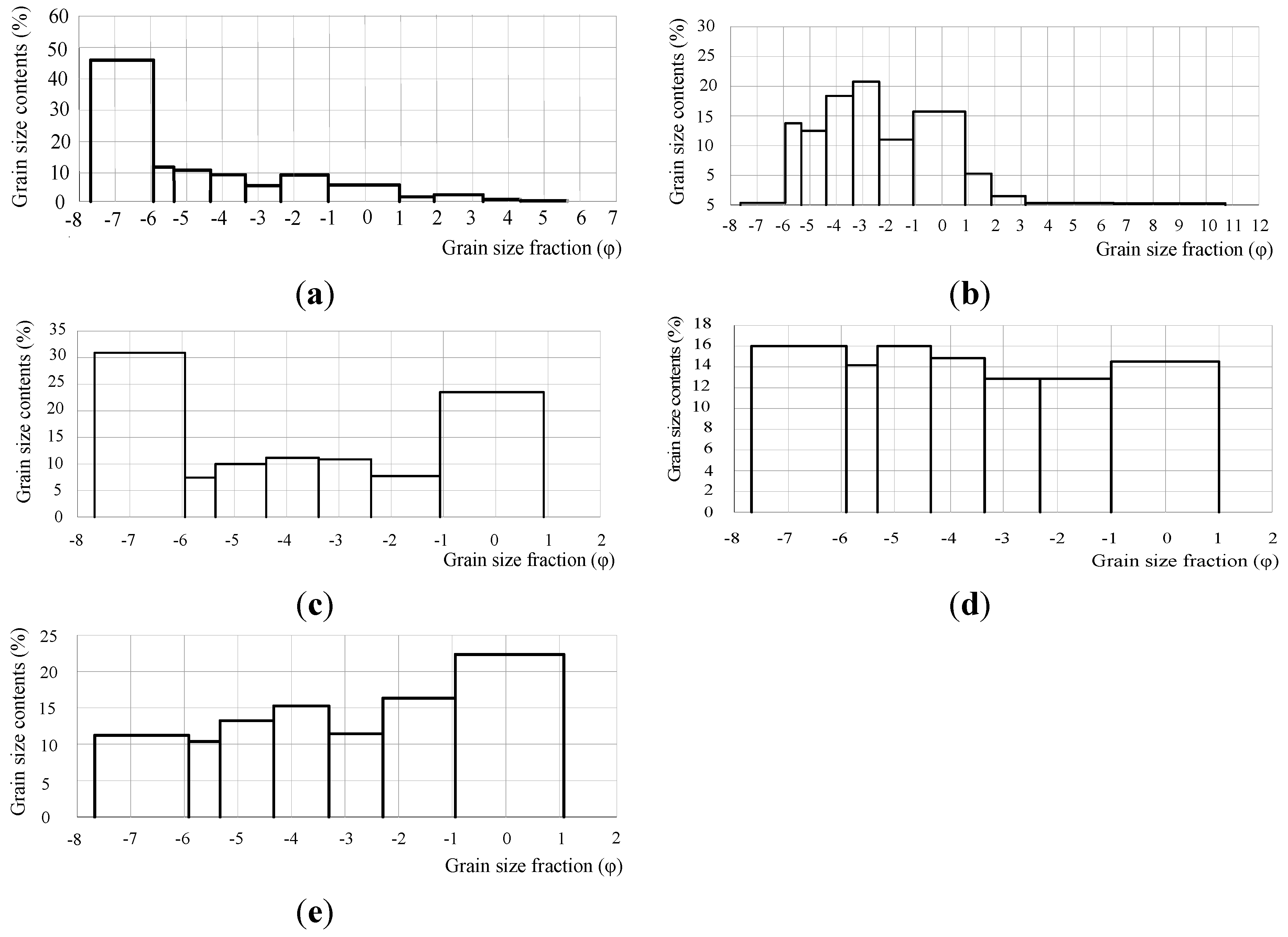
By means of the grain size analyses we have carried out, we have classified the studied debris flows into the five groups that are illustrated in Figure 10 and Table 6. Type I exhibits a shape of negative exponential density distribution, Type II features a normal or gamma density distribution shape, Type III has a letter U shape, Type IV shows a uniform density distribution shape, and Type V has a positive exponential density distribution shape. The different histogram shapes show different kinetic energy values, loose source material types, and grain-size distributions, among others.

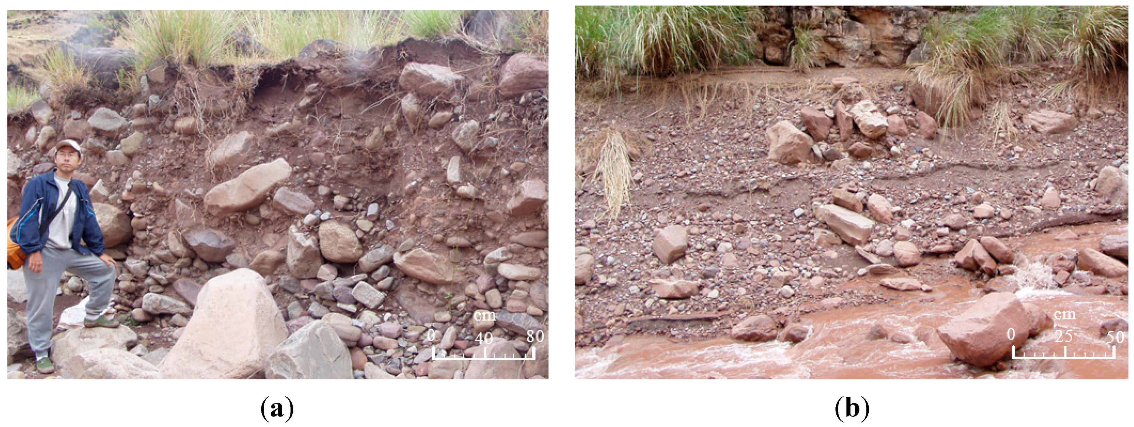
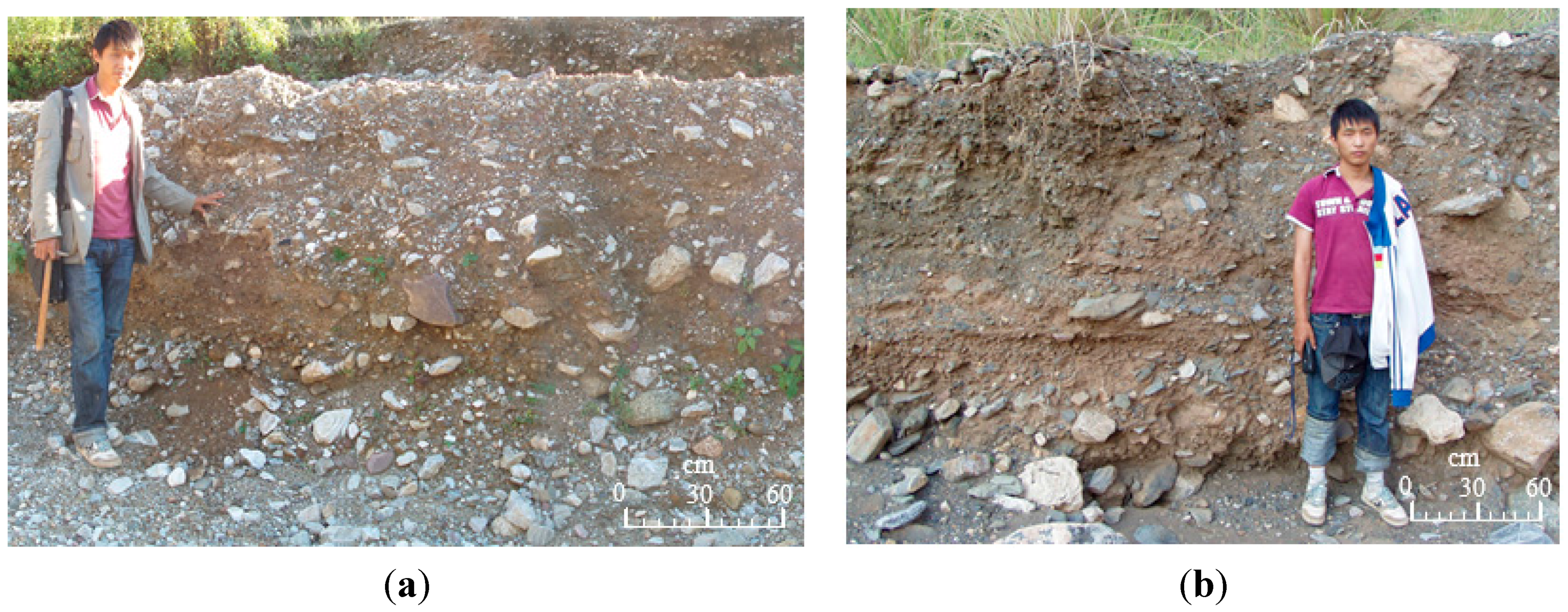
Figure 10. (a) A grain size distribution for debris flow Type I; (b) A grain size distribution for debris flow Type II; (c) A grain size distribution for debris flow Type III; (d) A grain size distribution for debris flow Type IV; (e) A grain size distribution for debris flow Type V. Five types of grain size distributions for debris flow materials.

Figure 10. (a) A grain size distribution for debris flow Type I; (b) A grain size distribution for debris flow Type II; (c) A grain size distribution for debris flow Type III; (d) A grain size distribution for debris flow Type IV; (e) A grain size distribution for debris flow Type V. Five types of grain size distributions for debris flow materials.

We have examined the degree of sorting of the deposits and because the larger the sorting, the larger the travel distance of the flows [29,30], we have included in Table 6 the potential travel distance that the flows would have had without entering the Jinsha river. However, the correlation we obtain where the mobility of the flows increases as the grain size decreases is confirmed by laboratory experiments [31] and numerical simulations [32].

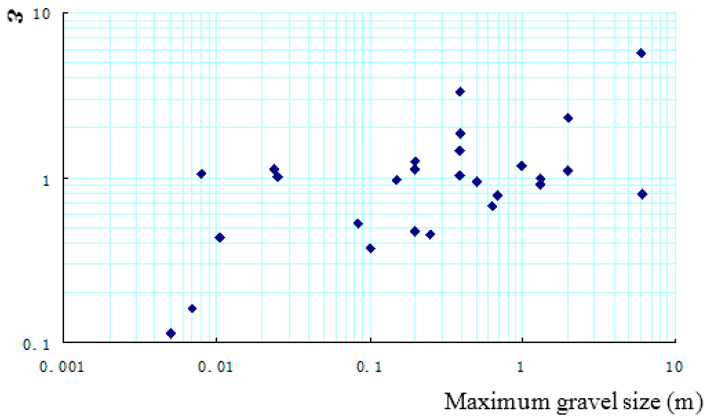
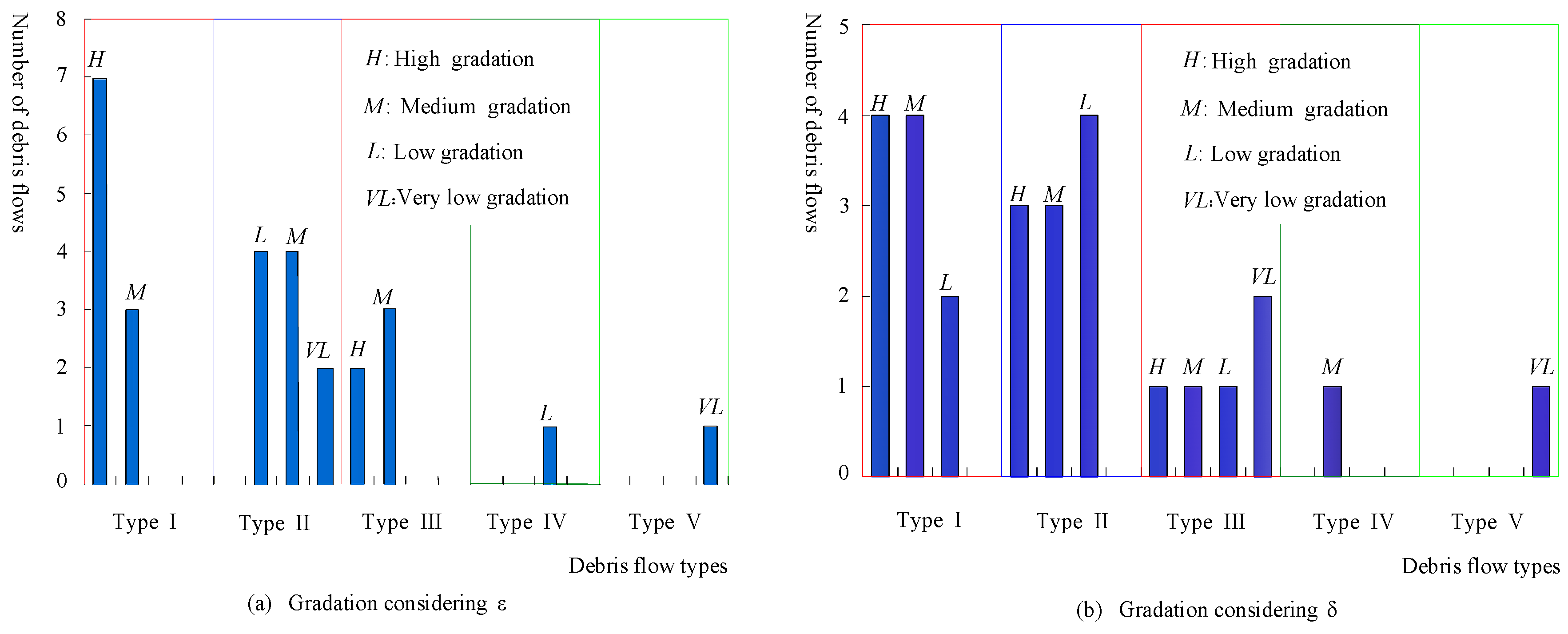
A grain index is recommended by the author to describe the characteristics of the debris-flow materials. The grain index ε is defined by Equation (6):

$$\text{ε}=\frac{\text{σ}\cdot SK}{Kg}{10}^{-(0.3M)}$$

(6)

where ε has a positive correlation with the mean grain size, standard deviation, and coefficient of skewness and has a negative correlation with the coefficient of kurtosis. A larger mean grain size (M) indicates the flow can carry a larger amount of sediment. A greater standard deviation indicates a poorer degree of sorting and a shorter transportation distance. A greater coefficient of skewness indicates a larger grain diameter. A greater coefficient of kurtosis indicates a narrower and sharper curve shape, which represents a better degree of sorting, longer transportation distance, and the less sediment the flow can carry. The flow with high transport energy can carry different sized gravels, which results in a large σ and a small Kg. Only the flow with a high velocity can carry large sized of gravels. A great proportion of large gravels result in large SK and M. Therefore, ε reflects the information on the debris flow transport (kinetic) energy, which represents the ability to carry poorly sorted sediment, especially large gravels. However, it is not strictly equal to the transport energy value stored in the debris flow. The value of the grain index for each debris flow was calculated by Equation (6) and is shown in Column 8 in Table 7.

Table 7. Grain index and normalized grain index for the 27 debris flow catchments.

Type	Debris Flow Catchment	M 1	D 2 (mm)	σ 3	Sk 4	Kg 5	ε 6	S 7	δ 8
I	Xiabaitan	−5.03	32.28	2.19	0.40	1.04	27.19	3.1	8.77
	Shangbaitan	−4.96	30.76	2.28	0.39	1.18	23.18	0.91	25.47
	Zhugongdi	−4.91	29.72	2.07	0.27	0.93	17.86	6.5	2.75
	Menggu	−4.80	27.54	2.08	0.41	1.26	18.64	37.1	0.50
	Kuashan	−4.68	25.35	2.41	0.40	0.88	27.77	6.66	4.17
	Yanshuijin	−4.95	30.55	2.60	0.53	1.10	38.27	48.58	0.79
	Zhili	−5.03	32.28	2.04	0.34	1.11	20.17	120.6	0.16
	Pingdi	−4.62	24.32	2.40	0.40	1.14	20.48	24.2	0.85
	Mutudahe	−4.68	25.35	2.61	0.43	1.31	21.72	98	0.22
	Fapa	−4.76	26.79	2.03	0.32	1.11	15.68	24.1	0.65
II	Yindigou	−3.63	12.27	2.23	0.18	0.71	6.94	60.5	0.11
	Xiushuihe	−4.11	17.10	2.12	0.38	0.95	14.50	8.58	1.69
	Nuozhami	−3.93	15.10	2.01	0.15	0.93	4.90	32.61	0.15
	Mapidi	−3.53	11.46	2.65	0.30	1.01	9.02	7.2	1.25
	Zhangmuhe	−3.49	11.14	1.82	0.15	0.70	4.35	4.62	0.94
	Hepiao	−3.70	12.88	2.04	0.24	0.96	6.57	9.1	0.72
	Jiaoping	−4.50	22.39	1.67	0.32	1.41	8.48	46.9	0.18
	Tianfanghe	−4.06	16.52	2.37	0.51	1.42	14.06	13.1	1.07
	Jiali	−4.36	20.32	2.12	0.34	1.00	14.65	18.9	0.78
	Daqing	−4.05	16.41	2.61	0.44	1.26	14.95	31.8	0.47
III	Jiachehe	−3.79	13.71	2.84	0.38	0.94	15.74	15.6	1.01
	Zhuzhahe	−4.44	21.48	3.23	0.64	0.84	52.85	152.6	0.35
	Yajiede	−4.06	16.52	2.81	0.46	0.97	22.01	22.3	0.99
	Chenhe	−4.34	20.04	2.26	0.30	0.99	13.73	590	0.02
	Mengguohe	−4.95	30.55	2.05	0.39	1.33	18.36	620.8	0.03
IV	Hujia	−3.77	13.52	2.46	0.24	1.05	7.60	8.62	0.88
V	Canyuhe	−3.11	8.57	2.62	0.15	0.94	3.58	256	0.01

¹ Mean grain size; ² Mean grain diameter; ³ Standard deviation; ⁴ Coefficient of Skewness; ⁵ Coefficient of Kurtosis; ⁶ Grain index; ⁷ Catchment area; ⁸ Normalized grain index.

Table 7. Grain index and normalized grain index for the 27 debris flow catchments.

Type	Debris Flow Catchment	M 1	D 2 (mm)	σ 3	Sk 4	Kg 5	ε 6	S 7	δ 8
I	Xiabaitan	−5.03	32.28	2.19	0.40	1.04	27.19	3.1	8.77
	Shangbaitan	−4.96	30.76	2.28	0.39	1.18	23.18	0.91	25.47
	Zhugongdi	−4.91	29.72	2.07	0.27	0.93	17.86	6.5	2.75
	Menggu	−4.80	27.54	2.08	0.41	1.26	18.64	37.1	0.50
	Kuashan	−4.68	25.35	2.41	0.40	0.88	27.77	6.66	4.17
	Yanshuijin	−4.95	30.55	2.60	0.53	1.10	38.27	48.58	0.79
	Zhili	−5.03	32.28	2.04	0.34	1.11	20.17	120.6	0.16
	Pingdi	−4.62	24.32	2.40	0.40	1.14	20.48	24.2	0.85
	Mutudahe	−4.68	25.35	2.61	0.43	1.31	21.72	98	0.22
	Fapa	−4.76	26.79	2.03	0.32	1.11	15.68	24.1	0.65
II	Yindigou	−3.63	12.27	2.23	0.18	0.71	6.94	60.5	0.11
	Xiushuihe	−4.11	17.10	2.12	0.38	0.95	14.50	8.58	1.69
	Nuozhami	−3.93	15.10	2.01	0.15	0.93	4.90	32.61	0.15
	Mapidi	−3.53	11.46	2.65	0.30	1.01	9.02	7.2	1.25
	Zhangmuhe	−3.49	11.14	1.82	0.15	0.70	4.35	4.62	0.94
	Hepiao	−3.70	12.88	2.04	0.24	0.96	6.57	9.1	0.72
	Jiaoping	−4.50	22.39	1.67	0.32	1.41	8.48	46.9	0.18
	Tianfanghe	−4.06	16.52	2.37	0.51	1.42	14.06	13.1	1.07
	Jiali	−4.36	20.32	2.12	0.34	1.00	14.65	18.9	0.78
	Daqing	−4.05	16.41	2.61	0.44	1.26	14.95	31.8	0.47
III	Jiachehe	−3.79	13.71	2.84	0.38	0.94	15.74	15.6	1.01
	Zhuzhahe	−4.44	21.48	3.23	0.64	0.84	52.85	152.6	0.35
	Yajiede	−4.06	16.52	2.81	0.46	0.97	22.01	22.3	0.99
	Chenhe	−4.34	20.04	2.26	0.30	0.99	13.73	590	0.02
	Mengguohe	−4.95	30.55	2.05	0.39	1.33	18.36	620.8	0.03
IV	Hujia	−3.77	13.52	2.46	0.24	1.05	7.60	8.62	0.88
V	Canyuhe	−3.11	8.57	2.62	0.15	0.94	3.58	256	0.01

¹ Mean grain size; ² Mean grain diameter; ³ Standard deviation; ⁴ Coefficient of Skewness; ⁵ Coefficient of Kurtosis; ⁶ Grain index; ⁷ Catchment area; ⁸ Normalized grain index.

Table 6 shows the grain size data for each debris flow catchment investigated in situ. Both Types I and II have ten debris flows, Type III has five debris flows, and Types IV and V have only one debris flow each.

5. Analysis

5.1. Grain Index (ε)

Table 6 shows that the average d values are approximately 28.5, 20.5, 15.6, 13.5, and 8.6 mm for Types I, III, II, IV, and V, respectively. Larger values indicate higher kinetic energies of debris flows, which is similar to the findings of Wang [22] and Zhang et al. [23]. Type I has the highest transport energy, followed by Types II and III, and then Type V. The degree of sorting can be evaluated by the standard deviation shown in Table 2 [28,33]. Most of the samples show gradation with a very poor degree of sorting, and few samples are extremely poor or poor. Most of the samples are extremely positively skewed, and a few are positively skewed. The kurtosis values of the samples indicate moderate to narrow and sharp forms, and a few indicate wide and gentle forms.

Equation (6) defined the grain index (ε). A larger ε indicates a debris flow with greater transport energy. This equation considers the grain size data including its distribution shape and the mean grain size, which corresponds to references [19,20,21]. Table 6 shows that ε ranges from approximately 3.6 to 53, with the highest value in Type III and the lowest value in Type V. The grain index values for Types I and III are almost at the same level, which is greater than those of Types II, IV, and V. ε is only related to the characteristics of the accumulation fan (i.e., the parameters from the grain-size distribution analysis). To comprehensively reflect the characteristics of the debris-flow materials, the next section proposes a new parameter named normalized grain index (δ).

5.2. Normalized Grain Index (δ)

The grain-size distribution reflects the transportation parameters (e.g., transport distance and transport channel width). The transportation parameters vary significantly in different debris flow catchments with different catchment areas. A study of 219 debris flow catchments in Gansu Province [34] shows that debris flow activity was clearly related to the catchment area. The ratios of the numbers of debris flow catchments to the total number of catchments for catchment area ranges are as follows: <0.5 km² is 11.9%, 0.5 km²–10 km² is 61.6%, 10 km²–50 km² is 22.4%, 50 km²–100 km² is 3.2%, and 100 km²–500 km² is 0.9%. The relationship is explained as follows: when a catchment area is <0.5 km², the quantity of rainwater is too small to initiate debris flows. When the catchment area is 0.5 km²–10 km², the confluent flow rate is sufficient to initiate debris flows; thus, the frequency is highest in catchments of this size. When the catchment area is 10 km²–50 km², the confluent flow rate is large enough to form floods instead of debris flows; thus, the debris flow frequency is relatively small. When the catchment area is >50 km², the confluent flow rate is very large, which mostly causes floods; thus, debris flow activity becomes very low.

The kinetic energy of a debris flow is related to its catchment area. A larger area is characterized by a gentler and broader channel and a less steep mountain slope, resulting in a smaller amount of available kinetic energy for debris flows. The new concept of a normalized grain index δ, which is a measure of the grain index per unit area, is proposed as Equation (7):

$$\text{δ}=\frac{\text{ε}}{S}$$

(7)

where S is the catchment area (km²). Table 6 lists the calculated δ for each debris flow.

The alluvial fan characteristics depend on the characteristics of the feeder basin. Determining the normalized grain index δ using the feeder basin area is reasonable. The catchment area shows a positive correlation with and is much easier to determine than the feeder basin area.

The ε and δ values listed in Table 6 can be classified into four gradations (Table 7). Both ε and δ reflect the gradation of the debris flow characteristics. Based on the gradation in Table 8, they are marked in grey levels for ε and δ.

Table 8. Gradation of fluid dynamic characteristics.

Gradation	High	Medium	Low	Very Low
Grain index ε	>20	10–20	5–10	<5
Normalized grain index δ	>1	0.5–1	0.1–0.5	<0.1

Table 8. Gradation of fluid dynamic characteristics.

Gradation	High	Medium	Low	Very Low
Grain index ε	>20	10–20	5–10	<5
Normalized grain index δ	>1	0.5–1	0.1–0.5	<0.1

According to Zhou et al. [35], three factors (i.e., abundant loose materials, sufficient water, and suitable slope angles) are fundamental prerequisites for a debris flow to occur. The intensity values of the three factors affect the debris flow. Loose materials and water can be considered in the estimation of debris flow density. The grain-size distribution can be used to consider the characteristics of the debris-flow materials, which reflects the debris flow density. The catchment area usually shows a negative correlation to the slope of the debris flow channel. Therefore, the debris flow transport energy can be rationally reflected through the grain size parameters and the size of catchment area.

5.3. Analysis Related to the Catchment Area

The catchment areas for the 27 debris flow catchments investigated in the study region vary widely from around 1 to 621 km² (Table 6).To identify the differences in the characteristics of the debris flow materials, the 27 debris flows were divided into four categories based on the size of catchment area as described in the following sections.

5.3.1. Catchment Areas Larger than 100 km²

Debris flow catchments Zhili in Type I, Zhuzhahe, Chenhe, and Mengguohe in Type III, Canyuhe in Type V, and all the other large-scale tributaries of the Jinsha River have catchment areas in excess of 100 km². Accumulation fans have not developed at the Longchuanjiang and Yalongjiang estuaries. These two tributaries are the largest in the study region, with catchment areas greater than 1000 km² and lengths more than 100 km. Only fine sand is found in the estuaries. The accumulation fans of the other three main tributaries (Chenhe, Mengguohe, and Canyuhe) can be observed (Table 6).The catchment areas of these three tributaries are smaller than the abovementioned two tributaries but are still larger than 250 km². Table 6 shows that the values of ε are approximately 4–18, which indicates very low to medium gradations. The values of δ are 0.01–0.03, which indicates very low gradation. The catchment areas in Zhili and Zhuzhahe (121 km² and 153 km², respectively) are smaller than the five main tributaries. The values of ε for these two catchments are 20 and 53, respectively, which indicates medium to high gradations. Similarly, the values of δ for these two catchments are 0.16 and 0.35, respectively, which indicates low gradation.

Figure 11 shows the natural profiles of the alluvial fans for Mengguohe and Zhuzhahe with the catchment areas larger than 100 km².The debris grains are well sorted, and the sphericity is subrounded to rounded.

Figure 11. Natural profiles of the alluvial fans for (a) Mengguohe and (b) Zhuzhahe catchments.

Figure 11. Natural profiles of the alluvial fans for (a) Mengguohe and (b) Zhuzhahe catchments.

Comparison of the value of ε with that of δ clearly shows that δ is more reasonable to use in the evaluation of the extremely large-area debris flows.

5.3.2. Catchment Area of 50 km² to 100 km²

Only two debris flow catchments in the study region fall into the 50–100 km² category. The ε values for Mutudahe in Type I and Yindigou in Type II are approximately 22 and 7, respectively (Table 6), which indicate high and low gradations, respectively. The δ values are 0.22 and 0.11, respectively, and indicates low gradation, respectively.

The natural profiles of the alluvial fans of Mutudahe and Yindigou are shown in Figure 12. The debris grains are subrounded and poorly sorted. Vegetation covers are dense on the alluvial fans, indicating low debris flow frequencies. δ supports the geological evidence.

5.3.3. Catchment area of 10 km² to 50 km²

There are 11 debris flow catchments in this category: four debris flow catchments (Menggu, Yanshuijin, Pingdi, and Fapa) belong to Type I, five debris flow catchments (Nuozhami, Jiaoping, Tianfanghe, Jiali, and Daqing) belong to Type II, and two debris flow catchments (Jiachehe and Yanjinde) belong to Type III.

Table 6 shows that the ε values of approximately 16–38 and δ values of 0.65–2.75 correspond to the Type I debris flow catchments. ε and δ both indicate medium to high gradation. The ε values of approximately 5–15 and δ values of 0.15–1.07 correspond to the Type II debris flows. ε indicates low to medium gradation, and δ indicates low to high gradations. The ε values of about 16 and 22 and δ values of about 1.00 correspond to the Type III debris flow catchments. ε and δ both indicate medium and high gradations.

Figure 12. Natural profiles of the alluvial fans for (a) Mutudahe and (b) Yindigou catchments.

Figure 12. Natural profiles of the alluvial fans for (a) Mutudahe and (b) Yindigou catchments.

The natural profiles of the alluvial fans for Yanshuiing, Jiali, and Yajiede catchments are presented in Figure 13. The average grain diameters in Yanshuijing (Type I) are noticeably larger than those in Jiali (Type II) and Yajiede (Type III). The roundness of the particles of all 11 debris flows is poor and almost at the same level.

Figure 13. Natural profiles of the alluvial fans for (a) Yanshuijin; (b) Jiali; and (c) Yajiede catchments. Yanshuijiin, Jiali, and Yajiede debris flows belong to Types I, II, and III, respectively.

Figure 13. Natural profiles of the alluvial fans for (a) Yanshuijin; (b) Jiali; and (c) Yajiede catchments. Yanshuijiin, Jiali, and Yajiede debris flows belong to Types I, II, and III, respectively.

The highest δ for the debris flows in Type I is Pindi, for those in Type II it is Tianfanghe, and for those in Type III it is at Jiachehe. The lowest δ for the debris flows in Type I is Menggu, for those in Type II it is Nuozhami, and for those in Type III it is Yanjinde. The geological observations of the accumulation fan and the calculated values from Equation (7) are coincident, which means that δ values are significant in evaluating the debris flows.

5.3.4. Catchment Area of 0.5 km² to 10 km²

This category contains nine debris flow catchments: four debris flow catchments (Xiabaitan, Shangbaitan, Zhugongdi, and Kuashan) belong to Type I, four debris flow catchments (Xiushuihe, Mapidi, Zhangmuhe, and Hepiao) belong to Type II, and one debris flow catchment (Hujia) belongs to Type IV.

Table 6 shows that the ε values of approximately 18–28 and δ values of approximately 3–25 correspond to the Type I debris flow catchments. Table 7 shows that the ε values indicate medium to high gradations, and the δ values indicate high gradation. The ε values of approximately 4–15 and δ values of approximately0.7–1.7 correspond to the Type II debris flow catchments. The ε values indicate very low to low gradations, and the δ values indicate medium to high gradations. The ε value of approximately 8 and δ value of approximately 0.9 correspond to the Type IV Hujia debris flow catchment. The ε value indicates low gradation, and the δ value indicates medium gradation.

The natural profiles of the alluvial fans for Zhangmuhe and Hujia catchments are shown in Figure 14. The degree of sorting and roundness of the grains in the alluvial fans are very poor. The site evidence shows that the higher transport energy of the debris flow material is generally in the sequences of Type I, Type II, and Type IV, which is coincident with the δ values listed in Table 6.

Figure 14. Natural profiles of the alluvial fans for (a) Zhangmuhe and (b) Hujia catchments.

Figure 14. Natural profiles of the alluvial fans for (a) Zhangmuhe and (b) Hujia catchments.

5.4. Analysis of the Five Debris Flow Types

A total of 236 debris flow catchments were found by interpreting the SPOT5 remote sensing images. Here, five debris flow catchments have catchment areas larger than 100 km², and six have catchment areas between 50 km² and 100 km², 32 have catchment areas between 10 km² and 50 km², 162 have catchment areas between 0.5 km² and 10 km², and 31 have catchment area of less than 0.5 km². Most of the debris flow catchments in the study region have catchment areas between 0.5 km² and 10 km², which represent 68.6% of the 236 debris flow catchments. Catchment areas between 10 km² and 50 km² represent 13.6%, catchment areas of less than 0.5 km² represent 13.1%, and catchment areas larger than 50 km² represent only 4.7%. Therefore, the debris flow catchments with catchment areas between 0.5 km² and 10 km² are the most prevalent catchments in the study region, and those with catchment areas between 10 km² and 50 km² are significant in the study region. Thus, 74% of the debris flow catchments with catchment areas between 0.5 km² and 50 km² were considered for investigation in situ.

The five types of debris flows summarized in Table 6 can be used to roughly classify the debris flows from the histogram derived from the grain-size distribution. The negative exponential-shaped histogram (Type I) indicates that the transportation distance is very short, and the sedimentation process is rapid. The normal or gamma density distribution-shaped histogram (Type II) indicates that the transportation distance is short, and derrick stones are broken into smaller grains; in addition, the sedimentation process is rapid. The positive exponential-shaped histogram (Type V) indicates that the transportation distance is long, and the sedimentation process is slow. The “U”-shaped histogram (Type III) reflects two kinds of sedimentation processes. The left side of the histogram is similar to the exponential one (Type I); the right side is similar to the positive exponential one (Type V). Coarse materials are deposited on the alluvial fan. As the debris flow catchment develops, fine grains are mainly deposited on the alluvial fan.

The histogram types (Table 6) only roughly describe the features of the debris flows. To describe the characteristics of the debris-flow materials, ε (which consists of four grain size parameters) and δ (which involves not only the grain size parameters but also the catchment area) are used. The results of the analyses based on ε and δ are quite different.

For Type I, seven debris flows have high gradation, and three debris flows have medium gradation based on ε (Figure 15a). Four, four, and two debris flows have high, medium, and low gradation respectively, based on δ (Figure 15b).

For Type II, four, four, and two debris flows have medium, low, and very low gradation respectively, based on ε (Figure 15a). Three, three, and four debris flows have high, medium, and low gradation respectively, based on δ (Figure 15b).

For Type III, two debris flows have high gradations, and three have medium gradations respectively, based on ε (Figure 15a). One, one, and two debris flows have high, medium, and low gradation respectively, based on δ (Figure 15b).

For Type IV, the debris flow has low gradation based on ε and has a medium gradation based on δ (Figure 15a). For Type V, the debris flow has a very low gradation based on both ε and δ (Figure 15b).

The transport energy of the debris flow is related to the maximum gravel size in the accumulation zone. Zhang et al. [23] stated that the velocity, which represents the transport energy of a debris flow, is proportional to the square root of the maximum gravel size. We analyzed the relationship between ε and the maximum gravel size for the 27 catchments (Figure 16). A bi-logarithm coordinate system was used, the results shown that ε approximately increased with the maximum gravel size. This is reasonable because great debris flow transport energy can transport large gravel; thus, the calculation method of debris flow in this study was validated.

Figure 15. Gradations considering δ. Gradations for debris flow catchments considering (a) ε and (b) δ.

Figure 15. Gradations considering δ. Gradations for debris flow catchments considering (a) ε and (b) δ.

Figure 16. Maximum gravel size in accumulation zones for the 27 debris flow catchments.

Figure 16. Maximum gravel size in accumulation zones for the 27 debris flow catchments.

6. Conclusions and Suggestions

In the study region, 27 large-scale debris flow catchments from the 236 debris flow catchments along the Jinsha River have been investigated in situ. Coarse granular sieve analysis in situ, laboratory particle size analysis, and image analysis were performed on the grains in each accumulation fan.

The grain size distributions of the 27 debris flow materials vary significantly, which reflects different transport energies of the debris flows. In this study, five types of debris flows were classified. To quantitatively reflect the transport energy information, a new parameter (grain index) was proposed based on grain size data (mean grain size, standard deviation, coefficient of skewness, and coefficient of kurtosis).

Transport energy of a debris flow is related to the size of the catchment. Another parameter, normalized grain index involving the grain index and the catchment area, was proposed. Through the analysis of the 27 debris flow catchments, the two proposed parameters are appropriate to reflect the transport energy and sedimentary transport feature. The normalized grain index is better than the grain index in evaluating the characteristics of the debris-flow materials because the former factor corresponds better to the grain features of the debris flow materials.

References

1. Yin, Y.P. Features of landslides triggered by the Wenchuan earthquake. J. Eng. Geol. 2009, 17, 29–38. [Google Scholar]
2. Tang, C.; Zhu, J.; Li, W.L.; Liang, J.T. Rainfall-triggered debris flows following the Wenchuan earthquake. Bull. Eng. Geol. Environ. 2009, 68, 187–194. [Google Scholar] [CrossRef]
3. Lin, C.W.; Shieh, C.L.; Yuan, B.D.; Shieh, Y.C.; Liu, S.H.; Lee, S.Y. Impact of Chi-Chi earthquake on the occurrence of landslides and debris flows: Example from the Chenyulan River watershed, Nantou, Taiwan. Eng. Geol. 2003, 71, 49–61. [Google Scholar] [CrossRef]
4. Wan, S.; Lei, T.C.; Huang, P.C.; Chou, T.Y. The knowledge rules of debris flow event: A case study for investigation Chen Yu Lan River, Taiwan. Eng. Geol. 2008, 98, 102–114. [Google Scholar] [CrossRef]
5. Zhang, X.; Zhang, S.X.; Wang, S.X. Negative dislocation model of vertical crustal movement and background before Wenchun and Panzhihua earthquakes. J. Geod. Geodyn. 2009, 29, 16–22. [Google Scholar]
6. Cui, P.; Wen, L.K.; Xiang, L.Z. ENSO Impacts on Debris Flows in Xiaojiang River Basin. Adv. Clim. Chang. Res. 2011, 7, 342–348. [Google Scholar]
7. Chen, J.C.; Jan, C.D.; Huang, W.S. Characteristics of rainfall triggering of debris flows in the Chenyulan watershed, Taiwan. Nat. Hazards Earth Syst. 2013, 13, 1015–1023. [Google Scholar] [CrossRef]
8. Whipple, K.X.; Dunne, T. The influence of debris-flow rheology on fan morphology, Owens Valley, California. Geol. Soc. Am. B 1992, 104, 887–900. [Google Scholar] [CrossRef]
9. Boniello, M.A.; Calligaris, C.; Lapasin, R.; Zini, L. Rheological investigation and simulation of a debris-flow event in the Fella watershed. Nat. Hazards Earth Syst. 2010, 10, 989–997. [Google Scholar] [CrossRef]
10. Kean, J.W.; Staley, D.M.; Cannon, S.H. In situ measurements of post fire debris flows in southern California: Comparisons of the timing and magnitude of 24 debris flow events with rainfall and soil moisture conditions. J. Geophys. Res. 2011. [Google Scholar] [CrossRef]
11. Rogers, R.R. Fine-grained debris flows and extraordinary vertebrate burials in the Late Cretaceous of Madagascar. Geology 2013, 33, 297–300. [Google Scholar] [CrossRef]
12. Ellen, S.D.; Fleming, R.W. Mobilization of debris flows from soil slips, San Francisco Bay Region, California, debris flows/avalanches: Process, recognition and mitigation. Rev. Eng. Geol. Geol. Soc. Am. 1987, 7, 31–40. [Google Scholar]
13. Blijenberg, H.M. Application of physical modeling of debris flow triggering to field conditions: Limitations posed by boundary conditions. Eng. Geol. 2007, 91, 25–33. [Google Scholar] [CrossRef]
14. Prochaska, A.B.; Santi, P.M.; Higgins, J.D.; Cannon, S.H. Debris-flow runout predictions based on the average channel slope. Eng. Geol. 2008, 98, 29–40. [Google Scholar] [CrossRef]
15. Iverson, N.R.; Mann, J.E.; Iverson, R.M. Effects of soil aggregates on debris-flow mobilization: Results from ring-shear experiments. Eng. Geol. 2010, 114, 84–92. [Google Scholar] [CrossRef]
16. Sumner, E.J.; Talling, P.J.; Amy, L.A. Deposits of flows transitional between turbidity current and debris flow. Geology 2009, 37, 991–994. [Google Scholar] [CrossRef]
17. Di Scotto Santolo, A.; Pellegrino, A.M.; Evangelista, A. Experimental study on the rheological behaviour of debris flow. Nat. Hazards Earth Syst. 2010, 10, 2507–2514. [Google Scholar] [CrossRef]
18. Bardou, E.; Boivin, P.; Pfeifer, H. Properties of debris flow deposits and source materials compared: Implications for debris flow characterization. Sedimentology 2007, 54, 469–480. [Google Scholar] [CrossRef]
19. Kokusho, T.; Hiraga, Y. Dissipated energies and friction coefficients in granular flow by flume tests. Soils Found. 2012, 52, 356–367. [Google Scholar] [CrossRef]
20. Federico, F.; Cesali, C. An energy-based approach to predict debris flow mobility and analyze empirical relationships. Can. Geotech. J. 2015. [Google Scholar] [CrossRef] [Green Version]
21. Tiranti, D.; Deangeli, C. Modeling of debris flow depositional patterns according to the catchment and sediment source area characteristics. Front. Earth Sci. 2015. [Google Scholar] [CrossRef]
22. Wang, Z.Y. Experimental study on debris flow head and the energy theory. J. Hydrol. Eng. 2001, 3, 18–26. [Google Scholar]
23. Zhang, S.X.; He, M.Y.; Xie, G.H. Calculation and analysis for super-huge types of debris flows in earthquake-stricken areas. Acta Geol. Sichuan 2014, 34, 36–44. [Google Scholar]
24. Zhang, W.; Li, H.Z.; Chen, J.P.; Zhang, C.; Xu, L.M.; Sang, W.F. Comprehensive hazard assessment and protection of debris flows along Jinsha River close to the Wudongde dam site in China. Nat. Hazard. 2011, 58, 459–477. [Google Scholar] [CrossRef]
25. Zhang, W.; Chen, J.P.; Wang, Q.; An, Y.K.; Qian, X.; Xiang, L.J.; He, L.X. Susceptibility analysis of large-scale debris flows based on combination weighting and extension methods. Nat. Hazards 2013, 66, 1073–1100. [Google Scholar] [CrossRef]
26. Tiranti, D.; Bonetto, S.; Mandrone, G. Quantitative basin characterization to refine debris-flow triggering criteria and processes: An example from the Italian Western Alps. Landslides 2008, 5, 45–57. [Google Scholar] [CrossRef]
27. Krumbein, W.C. Application of logarithmic moments to size frequency distributions of sediments. J. Sediment. Res. 1936, 6, 35–47. [Google Scholar] [CrossRef]
28. Folk, R.L.; Ward, W.C. Brazos river bar: A study in the significance of grain size parameters. J. Sediment. Res. 1957, 27, 3–26. [Google Scholar] [CrossRef]
29. Zhang, L.M.; Xu, Y.; Huang, R.Q.; Chang, D.S. Particle flow and segregation in a giant landslide event triggered by the 2008 Wenchuan earthquake, Sichuan, China. Nat. Hazards Earth Syst. 2011, 11, 1153–1162. [Google Scholar] [CrossRef]
30. Coe, J.A.; Kinner, D.A.; Godt, J.W. Initiation conditions for debris flows generated by runoff at Chalk Cliffs, central Colorado. Geomorphology 2008, 96, 270–297. [Google Scholar] [CrossRef]
31. Cagnoli, B.; Romano, G.P. Granular pressure at the base of dry flows of angular rock fragments as a function of grain size and flow volume: A relationship from laboratory experiments. J. Geophys. Res. 2012, 117, B10202. [Google Scholar] [CrossRef]
32. Cagnoli, B.; Piersanti, A. Grain size and flow volume effects on granular flow mobility in numerical simulations: 3-D discrete element modeling of flows of angular rock fragments. J. Geophys. Res. Solid Earth 2015, 120, 2350–2366. [Google Scholar] [CrossRef] [Green Version]
33. Johnson, K.G.; Friedman, G.M. The Tully clastic correlatives (Upper Devonian) of New York State; a model for recognition of alluvial, dune, tidal, nearshore (bar and lagoon) and offshore sedimentary environments in a tectonic delta complex. J. Sediment. Res. 1969, 39, 451–485. [Google Scholar]
34. Lu, R.R. An analysis of differentiation factors of debris flow gully. Mt Res. 1985, 3, 121–128. [Google Scholar]
35. Zhou, B.F.; Lee, D.J.; Luo, D.F.; Lu, R.R.; Yang, C.S. A Guide for Debris-Flows Hazard Mitigation; Science Publisher: Beijing, China, 1991. (In Chinese) [Google Scholar]