Risk Assessment, Partition and Economic Loss Estimation of Rice Production in China

Abstract

Agricultural risk, especially the risk assessment, partition and economic loss estimation of specific and main crops, maize, wheat and rice, is widely touted in China as a means of improving the effective productivity. The main objective of this article is to perform a detailed analysis of the stability and comparative advantage of rice production in 30 provinces on the basis of relative rice production data from 2000 to 2012 in China. The non-parametric information diffusion model based on entropy theory was used to assess rice production risk. Accordingly, we divided the risk level with hierarchical cluster analysis. Then, we calculated the economic loss of rice production by the scenario analysis. The results show that, firstly, the national disaster risk of rice production is at a lower level. Secondly, there are significant differences in the stability, comparative advantage and risk probability of rice production among the 30 provinces. Thirdly, Shanxi province belongs to the high risk zone, 12 provinces belong to the middle risk zone and 17 provinces to the low risk zone. Finally, there is a proportional rate between the economic loss (yield loss) and disaster area (yield loss rate) of rice production. Therefore, we could obtain some significant policy suggestions.

1. Introduction

Agriculture is the foundation of the development of the national economy. It plays an important role in the development of industry and the service industry. It is worthy of the consideration that China is an agricultural country. It is a wonder that we use 7% of the world’s cultivated land to raise about 20% of the world’s population. We are the eleventh in the uninterrupted growth of crop production from 2004. The crop production has surpassed 600 million tons for two years until 2014. However, the development of agriculture is still in the transition period of traditional to modern agriculture. The risk of agricultural production cannot be ignored. Agricultural production is faced with the double constraints of resources and markets, the dual pressure of economic growth and ecological protection and the double challenges of farmer’s income and food security in China. Therefore, it is significantly important to study the agricultural risk under the new challenges and changes in agricultural development.

Risk management originated in Germany after World War I [1]. Through a variety of forms, such as academic meetings or seminars, risk management began to catch on around the world in the 1980s. China began to introduce risk theory after the late 1980s, being slightly behind in theory research. On the whole, risk research has focused on four aspects: the concept [2], classification [3], evaluation [4,5] and management strategy [6].

Agricultural risk has always been an important issue in agricultural economic management. The study of agricultural risk is an irreplaceable part of risk research. Some previous studies have focused on the ecological risk management [7], such as soil fertility loss [8], water pollution [9,10] and pesticide risk [11]. Some relevant research has studied the food safety problem [12], e.g., crop production risk [13], genetically-modified food [14], invasive plants [15], and so on. Others refer to agricultural natural disaster risk, for example crop frost disaster risk [16], drought disaster risk [17], agricultural catastrophe [18], as well as meteorological disaster risk [19], such as flood risk [20] and large coastal storm surges [21,22].

From the study approach’s perspective, there are two categories included: the parameter estimation method and the non-parametric estimation method. From the perspective of risk partition, this refers to three research directions. First is the use of GIS technology [23], the natural disaster risk index method and the flood risk assessment model to discuss relative subjects and most using the weighted comprehensive evaluation method [24] and the fuzzy metrics method [25]. Second is the use of the overlay analysis function of software (such as Arcview, etc.) and the evaluation map to divide the disaster risk level in the study area [26]. Third is that the risk also could be partitioned by using cluster analysis according to the selected risk factors [27]. Then, for risk loss estimation, based on the risk assessment criteria, research has followed the computable general equilibrium model [28], the input-output model [29] or scenario analysis [30], as well as other models or ways to assess direct (indirect) economic loss or integrated (economic, non-economic) loss.

The previous studies on disaster risk assessment have drawn some important conclusions to improve disaster prevention capability. Some research has established disaster prevention mechanisms to reduce agricultural risk loss in the future. However, there are less studies about crops, especially the specific risk research on food crops. From the risk assessment methods, researchers mostly have used the traditional non-parametric information diffusion model. In fact, we need to give more attention to the estimated result accuracy of the model. Furthermore, in risk zones and for loss estimations, the previous studies have a limited sample size and have always taken one province as the research area.

Rice plays a major role in the development of the agricultural economy, as it is one of the most important food crops in China. Its perennial cultivated areas and total production are ahead of other crops. Compared with other rice production countries, both the yield per unit area and the total output of rice are higher in China. With increasing levels of mechanization and integrated promotion and application of technology in agricultural production, rice production has improved greatly. However, every story has two sides. The risk is continuously increasing with the development of rice production. Unlike in the past, with the continual raising of natural resource constraints on rice production, current rice production relies more heavily on the role of agricultural science and technology (AST) Rice production is more inclined toward intensive production which is more feasible and economic compared with the traditional, semi-wild extensive management of expanding land area.

Therefore, we took rice as the research object. Giving full consideration to the influence of AST, we calculated the loss rate of the yield unit area according to the reference data selected from the China statistical yearbook and China rural statistical yearbook from 2000 to 2013 [31,32]. Then, we established a non-parametric information diffusion model based on entropy theory to assess the rice production risk in 30 provinces (without including Taiwan and Qinghai provinces due to the status of rice production and the availability of data). Accordingly, while combining with hierarchical cluster analysis, we divided the rice risk level. Finally, we used the scenario analysis method to assess the risk of economic loss.

The paper is structured as follows. Section 2 introduces the research methods and models. Section 3 analyzes the status of rice production in China. Empirical results are presented and discussed in Section 4. Section 5 provides the conclusions and future research directions.

2. Research Methodologies

With full consideration of the research perspective and the availability of research data, we did not describe risk from the micro perspective (i.e., farm-level data). In particular, we noted that the analysis data were referenced to the province level data in this research based on the analysis framework of a medium-level perspective. The research sample is a total of 390, consisting of 30 provinces with 13 years of data. As for the research methods, we give the practicability and the reasons why we chose the methods before introducing these methods. The relevant details are listed before every method.

2.1. Coefficient of Variation

The coefficient of variation is a statistical way to measure the variability of the observed values. It can eliminate the effects of two or more data variations caused by the different units and the average. We used it to measure the stability of rice yields in the 30 provinces. The derivation of the formula is as follows,

$$C.V{.}_i=\raisebox{1ex}{$S_i$}\!\left/ \!\raisebox{-1ex}{${\overline{x}}_i$}\right.$$

(1)

where $C.V{.}_i$ is the coefficient of variation, $S_i$ is the standard deviation and ${\overline{x}}_i$ is the average of the rice yields in region i.

$$S_i=\sqrt{{\displaystyle \sum {\left(x_i-{\overline{x}}_i\right)}^2}}/\left(m-1\right)$$

(2)

where $i=1,2,\cdots ,30$ means 30 provinces in China and $m=13$ expresses the sample size of $x_i$.

2.2. Comparative Advantage Index

The comparative advantage index includes the scale advantage, efficiency and comprehensive superiority index. They usually are used as a way to analyze crop scale, land productivity and comprehensive production advantage in a certain range. The comprehensive superiority index is the consolidated results of the efficiency and scale advantage index. Therefore, it is better to show the comprehensive advantage in a certain area. Hence, we used it as an indicator of the rice production risk zone in China. Its formula is as follows:

$$Z{H}_{ij}=\sqrt{G{M}_{ij}·S{G}_{ij}}$$

(3)

where $Z{H}_{ij}$ is the comprehensive superiority index of crop $j$ in region $i$. The region has a comprehensive comparative advantage of the crop when $Z{H}_{ij}\ge 1$. The advantage would be more obvious as $Z{H}_{ij}$ becomes larger and larger. Similarly, the region does not have the advantage when $Z{H}_{ij}<1$.

$G{M}_{ij}$ is the scale advantage index of crop $j$ in region $i$. The index can reflect the production scale and the specialization degree in this region. The formula is as follows,

$$G{M}_{ij}=\frac{S_{ij}/S_i}{S_j/S}$$

(4)

where $S_{ij}$ is the cultivated area of crop $j$ and $S_i$ is the total crop area in region $i$. $S_j$ is the total cultivated area of crop $j$, and $S$ is the total acreage of all of the crops in the whole country. Normally, we assumed that region $i$ has the specialization advantage of crop $j$ when $G{M}_{ij}\ge 1$ and that the specialization degree would become higher and higher according to the increasing of $G{M}_{ij}$. This means that the region does not have the advantage and is not even good for planting the crop when $G{M}_{ij}<1$. Similarly, the advantage becomes smaller and smaller as $G{M}_{ij}$ reduces.

$S{G}_{ij}$ is the comparative advantage index of the production level, and it can reflect the land productivity of crop $j$ in region $i$. We can get SG_ij by comparing the crop yield in the research area with the national average level. The formula is as follows,

$$S{G}_{ij}=\frac{G_{ij}/Y_{ij}}{G_j/Y_j}$$

(5)

where $G_{ij}$ is the production and Y_ij is the cultivated area of crop j in region i. $G_j$ and Y_j are the corresponding values of the whole country. The region has a high crop production ability and output rate when $S{G}_{ij}\ge 1$, and the production rate becomes higher and higher as SG_ij increases. Instead, the region does not have the advantage as SG_ij ˂ 1.

2.3. Risk Assessment Model

As we discussed above, the methods of risk assessment consisted of parameter and non-parameter estimation. However, we must know the distribution model of research data when using the parameter estimation method. Otherwise, it would take much time to fit the sample many times to choose the right distribution model. In contrast, we can use the non-parameter estimation method directly without considering the status of the sample distribution. What is more, it is also conducive to operate on and analyze small samples. As a famous non-parameter estimation method, the information diffusion model not only has the characteristics of the non-parameter estimation method, but also has the function of the fuzzy mathematical method. Combined with the features of the research subject and sample, we took the information diffusion model as the main way to assess risk.

We need to diffuse the limited sample information to get more accurate results. According to the information diffusion theory of Huang [33], we give the following detailed formulas. Firstly, we assumed that sample set $X$ diffused its information to all of the points of the set $U$ based onEquation (6).

$$f_i\left(u_j\right)=\frac{1}{h\sqrt{2\pi }}\exp \left(-\frac{{\left(x_i-u_j\right)}^2}{2h^2}\right)$$

(6)

where $U=\left\{u_1,u_2,\cdots u_{j-1},u_j,u_{j+1},\cdots ,u_n\right\}$ is the index diffusion set into which every $x_i$ can diffuse information. The step of U can be set due to the size of the research sample. In our study,

$$U=\left\{0,0.01,0.02\cdots ,1\right\}$$

(7)

The traditional way of computation was determined by the empirical formula, so that it lacked an adequate theoretical basis with the precision limited to a great extent. In order to improve the stability of the model, we used the improved method to calculate the information diffusion coefficient $h$, owing to having a direct impact on the effect and application of the model.

We introduced the information entropy of Claude [34]. Its formula is as follows,

$$H=-{\displaystyle \sum _{i=1}^m{p}_i\ln p_i}$$

(8)

Combined with Formula (6) and the maximum entropy principle, we can get the max entropy $H$ of the information diffusion function with a one-dimensional normal distribution (Formula (9)).

$$H=H\left(x\right)={\displaystyle \int \frac{1}{\sqrt{2\pi }\sigma }}\exp \left(-\frac{x^2}{2{\sigma }^2}\right)·\left(\ln \sqrt{2\pi }\sigma +\frac{x^2}{2{\sigma }^2}\right)dx=\ln \sqrt{2\pi e}\sigma$$

(9)

When the entropy reaches its maximum value,

$$H=-{\displaystyle \sum _{i=1}^m{p}_i\ln p_i}=\ln \left(m\right)$$

(10)

Based on the Formula (9),

$$\sigma =e^H/\sqrt{2\pi e}$$

(11)

Because $h=\sigma ·{\Delta }_m$, $b=\max \left\{x_{ij}\right\}$, $a=\min \left\{x_{ij}\right\}$ and ${\Delta }_m=\left(b-a\right)/\left(m-1\right)$ is the average step length, the formula of the information diffusion coefficient h based on the entropy theory are as follows:

$$h=\{\begin{array}{ll}\left(e^H/\sqrt{2\pi e}\right)\left(b-a\right)/\left(m-1\right)& m>11\\ \left(e^H/\sqrt{2\pi e}\right)\left(b-a\right)& m\le 11\end{array}$$

(12)

Combined with Formula (6), the normalized information distribution of the sample $x_i$ can be written as:

$${\mu }_{x_i}\left(u_j\right)=\frac{f_i\left(u_j\right)}{{\displaystyle \sum _{j=1}^n{f}_i}\left(u_j\right)}$$

(13)

Then, assuming,

$$q\left(u_j\right)={\displaystyle \sum _{i=1}^m{\mu }_{x_i}\left(u_j\right)}$$

(14)

and:

$$Q={\displaystyle \sum _{j=1}^{n}q\left(u_j\right)}$$

(15)

The frequency of the sample falling into the $u_j$ as well as the probability estimates is:

$$p\left(u_j\right)=\frac{q\left(u_j\right)}{Q}$$

(16)

The probability estimation beyond u_j is:

$$p\left(u>u_j\right)=1-{\displaystyle \sum _{k=1}^j\left(u_k\right)}$$

(17)

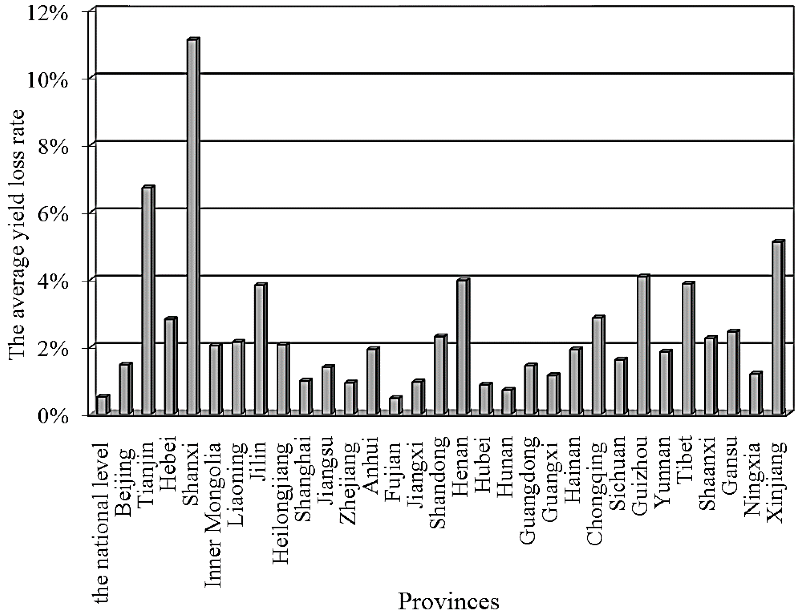
2.4. Yield Loss Rate

Giving full consideration of the growing natural constraints and the progress of AST, the loss rate of yield unit area was selected as the basic data to assess and partition the risk of the rice production in this paper. The yield loss rate is a ratio value. Its formula could be written as,

$$\text{yield loss rate }=\text{ Max }\left(\text{yield fitted value }-\text{ yield actual value},0\right)/\text{yield actual value}$$

(18)

We got the fitted value by fitting the actual value. Due to the complexity of rice production, the whole rice production system could be influenced by many factors. There were some factors that we knew (i.e., subsidy policy, national economic level, some input index, conditions of natural production, and so on). However, there were still some factors that are unknown.

GM (1, 1) (i.e., Grey Model) is an important basic forecast model in the Grey theory. The model was dedicated to the processing of the problems with a few data and poor information. Therefore, we used the GM (1, 1) model to get the yield fitted value. For the detail of the calculated formulas, we could refer to Chen [35]. As for Formula (18), we knew that there would be the probability of rice production risk when the fitted value surpassed the actual value of the rice yield unit area. Instead, the risk probability would be small.

3. Qualitative Analyses

Rice is always at the top with respect to other food crops in China, irrespective of the cultivated area or the total output. Its cultivated area accounted for 27.10% of the total cultivated areas of grain crops, and the proportion of the total output was up to 34.64% in 2012. However, the cultivated area of corn began to surpass rice, so that it has moved to second place since 2007. The total rice output also changed to second place in 2012. Analyzing the rural China statistics data, we found that there was an upward trend with the volatility of the yield unit area and the total output of the rice production. Although the average annual growth of the total output was only 0.64%, the average annual growth of the yield per unit area was much lower, exclusively 0.60% in China from 2000 to 2012.

In addition, with industrialization and urbanization, agricultural production faced some natural resource constraints. The phenomenon could be illustrated by the change of total cultivated area. The cultivated land was 130.0391 million hectares in 2006, and it was reduced by 6.39% in 2007, reaching 121.7352 million hectares. In recent years, it reduced to 121.7159 million hectares, even with a zero growth rate until now. Similarly, the proportion of the rice cultivated area and production accounted for the food crops showed a downward trend. The corresponding proportions were 27.62% and 40.66% in 2000 and reduced to 27.10% and 34.64% in 2012, of which the proportion of the total output fell as much as 14.80%.

With the above analysis, it was significant that we took the yield per unit area as the basic research data. The yield loss rate could show the rice production risk accurately under the new natural constraints and the popularization and application of AST. As shown in Figure 1, the rice yields had an upward trend with some fluctuations. The per unit area yield had a drop in 2003 with 6060.68 kg. Overall, the rise in the rate was not significant, with an average annual increase of 0.60%, from 6271.59 kg in 2000 to 6776.89 kg in 2012.

Figure 1. Rice yield trend in China from 2000 to 2012 (Note: hm is the short form of hectare in the figure).

Figure 1. Rice yield trend in China from 2000 to 2012 (Note: hm is the short form of hectare in the figure).

From the perspective of the yield loss rate, it showed that there were significant differences in the stability of the 30 provinces in China (Figure 2). From 2000 to 2012, there was a lower yield loss rate, which was 0.52% in the whole country. Hence, it proved that there was basic stability in the rice yield nationwide. In terms of provinces, compared with the average level of the whole country, Fujian province had a lower yield loss rate, which was 0.48%. However, other provinces had a high yield loss rate. The yield loss rates of Shanghai, Zhejiang, Fujian, Jiangxi, Hubei and Hunan were less than 1%. The rates of Beijing, Jiangsu, Anhui, Guangdong, Guangxi, Hainan, Sichuan, Yunnan and Ningxia Hui autonomous region were between 1% and 2%. The rates of Hebei, Inner Mongolia, Liaoning, Jilin, Heilongjiang, Shandong, Henan, Chongqing, Tibet, Shaanxi and Gansu fell from 2% to 4%. The rate of Guizhou province was slightly higher than 4%, reaching 4.08%. The rate of Xinjiang exceeded 5%, going to 5.12%. The rate of Tianjin was much higher, up to 6.73%. The rate in Shanxi province was the highest, attaining 11.12%.

Figure 2. The status of the rice yield loss rate in China from 2000 to 2012.

Figure 2. The status of the rice yield loss rate in China from 2000 to 2012.

4. Quantitative Analysis

4.1. Risk Assessment

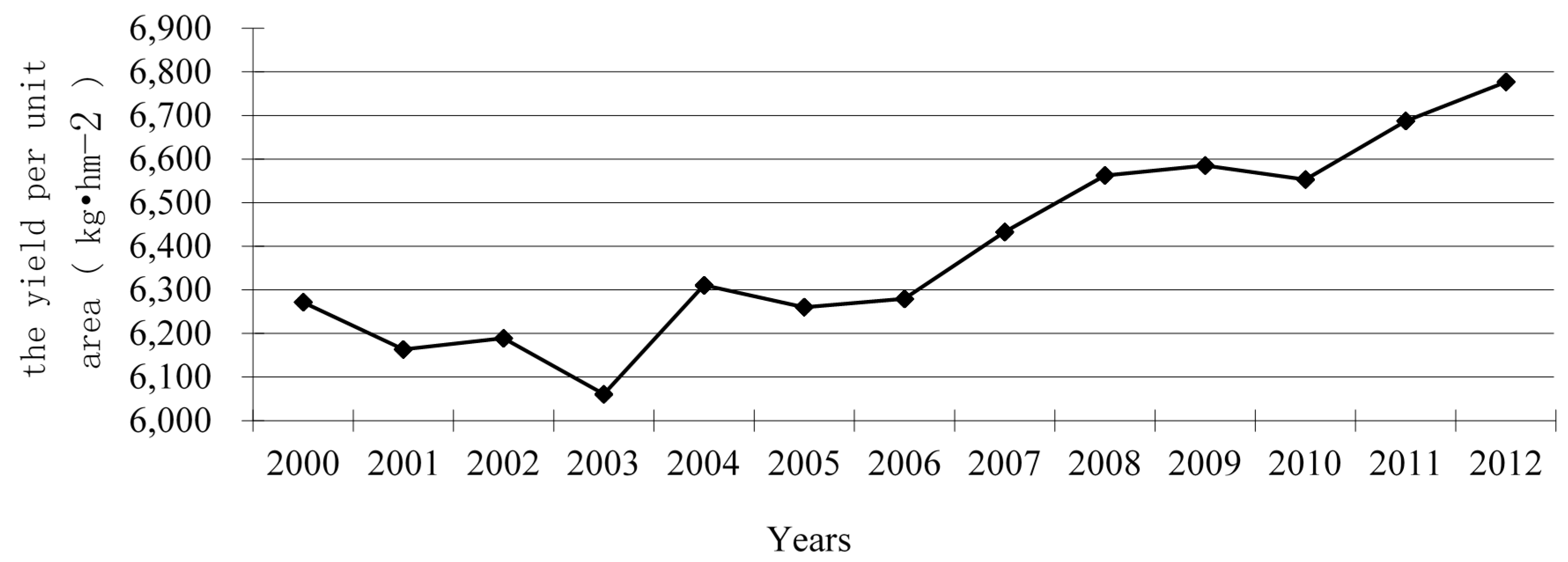
4.1.1. Stability Analysis

Combined with the Statistic Package for Social Science (SPSS) 17.0 and based on Formulas (1) and (2), we got the rice yield fluctuation status, as shown in Table 1. Overall, the coefficient of variation (C.V.) of the national rice yield was 0.0345. This showed that we had a relatively stable production level with a small fluctuation in the whole country. From the perspective of the 30 provinces, the C.V. in Hubei, Hunan, Ningxia and Shanghai was below the national level. Especially, Hunan’s C.V. reached a min value of 0.0234. The average fluctuation of the rice cultivated area and the total output were both lower than 0.80% in Hubei and Hunan. These values in Shanghai were both lower than 3.90%. The possible reason for the above results was that Hubei, Hunan and Shanghai, as the main double-crop or single-crop rice production provinces in central China, had a lower yield variation degree, because of relatively stable cultivated area and total output of rice production. As important early and medium rice production regions in the dry northwest region, Ningxia Hui autonomous region, including Yinchuan and Hetao plain, has always been famous as “Sai shang jiang nan”. It had a low level of variability in yield because its annual fluctuations of total rice cultivated area and production did not exceed 1%.

Table 1. The yield fluctuations in China from 2000 to 2012.

	The Min Yield	The Max Yield	The Average Yield	Standard Deviation (SD)	C.V.
The national level	6060.68	6776.89	6394.85	220.56	0.0345
Beijing	5750.00	6818.18	6336.47	265.91	0.0420
Tianjin	4096.05	8103.87	7087.68	1005.21	0.1418
Hebei	4572.62	7248.86	5967.72	846.22	0.1418
Shanxi	1228.07	7333.33	4512.17	1425.11	0.3158
Inner Mongolia	6097.97	8657.42	7153.66	803.49	0.1123
Liaoning	6502.42	7705.19	7320.37	417.37	0.0570
Jilin	5403.99	9019.90	7242.51	1159.40	0.1601
Heilongjiang	5887.24	7116.77	6564.55	356.76	0.0543
Shanghai	7583.42	8481.30	8100.12	276.60	0.0341
Jiangsu	7630.06	8626.71	8095.86	288.28	0.0356
Zhejiang	6196.50	7305.64	6784.23	349.82	0.0516
Anhui	4885.93	6494.30	6007.56	419.80	0.0699
Fujian	5148.21	6087.18	5648.71	335.49	0.0594
Jiangxi	5066.68	5936.91	5497.50	286.46	0.0521
Shandong	6266.97	8482.65	7732.91	841.07	0.1088
Henan	4774.75	7599.20	6879.96	933.51	0.1357
Hubei	7280.26	8183.74	7605.78	257.86	0.0339
Hunan	5983.91	6429.30	6219.01	145.57	0.0234
Guangdong	5153.32	5779.12	5441.36	201.06	0.0369
Guangxi	4768.25	5550.16	5180.46	204.47	0.0395
Hainan	3680.44	4801.55	4353.74	306.68	0.0704
Chongqing	5129.84	7859.82	6921.53	721.78	0.1043
Sichuan	6420.74	7695.17	7280.05	368.07	0.0506
Guizhou	4459.79	6671.53	6124.82	715.64	0.1168
Yunnan	5015.70	6229.17	5884.06	389.34	0.0662
Tibet	3529.41	6020.41	5436.21	654.36	0.1204
Shaanxi	5412.19	7082.43	6375.57	467.00	0.0732
Gansu	6458.33	9295.77	7625.35	871.78	0.1143
Ningxia	7862.34	8730.37	8322.80	263.88	0.0317
Xinjiang	5792.82	9273.73	7778.13	1099.02	0.1413

Note: the unit of yield in the table was kg·hm⁻².

Table 1. The yield fluctuations in China from 2000 to 2012.

	The Min Yield	The Max Yield	The Average Yield	Standard Deviation (SD)	C.V.
The national level	6060.68	6776.89	6394.85	220.56	0.0345
Beijing	5750.00	6818.18	6336.47	265.91	0.0420
Tianjin	4096.05	8103.87	7087.68	1005.21	0.1418
Hebei	4572.62	7248.86	5967.72	846.22	0.1418
Shanxi	1228.07	7333.33	4512.17	1425.11	0.3158
Inner Mongolia	6097.97	8657.42	7153.66	803.49	0.1123
Liaoning	6502.42	7705.19	7320.37	417.37	0.0570
Jilin	5403.99	9019.90	7242.51	1159.40	0.1601
Heilongjiang	5887.24	7116.77	6564.55	356.76	0.0543
Shanghai	7583.42	8481.30	8100.12	276.60	0.0341
Jiangsu	7630.06	8626.71	8095.86	288.28	0.0356
Zhejiang	6196.50	7305.64	6784.23	349.82	0.0516
Anhui	4885.93	6494.30	6007.56	419.80	0.0699
Fujian	5148.21	6087.18	5648.71	335.49	0.0594
Jiangxi	5066.68	5936.91	5497.50	286.46	0.0521
Shandong	6266.97	8482.65	7732.91	841.07	0.1088
Henan	4774.75	7599.20	6879.96	933.51	0.1357
Hubei	7280.26	8183.74	7605.78	257.86	0.0339
Hunan	5983.91	6429.30	6219.01	145.57	0.0234
Guangdong	5153.32	5779.12	5441.36	201.06	0.0369
Guangxi	4768.25	5550.16	5180.46	204.47	0.0395
Hainan	3680.44	4801.55	4353.74	306.68	0.0704
Chongqing	5129.84	7859.82	6921.53	721.78	0.1043
Sichuan	6420.74	7695.17	7280.05	368.07	0.0506
Guizhou	4459.79	6671.53	6124.82	715.64	0.1168
Yunnan	5015.70	6229.17	5884.06	389.34	0.0662
Tibet	3529.41	6020.41	5436.21	654.36	0.1204
Shaanxi	5412.19	7082.43	6375.57	467.00	0.0732
Gansu	6458.33	9295.77	7625.35	871.78	0.1143
Ningxia	7862.34	8730.37	8322.80	263.88	0.0317
Xinjiang	5792.82	9273.73	7778.13	1099.02	0.1413

Note: the unit of yield in the table was kg·hm⁻².

Yield variabilities in 14 provinces were lower than 7.50%, but higher than the national level, followed by Jiangsu, Guangdong, Guangxi, Beijing, Heilongjiang, Liaoning, Sichuan, Zhejiang, Jiangxi, Fujian, Yunnan, Anhui, Hainan and Shaanxi. Among them, the C.V. in Jiangsu was 0.0356, slightly above the national level. Guangdong, Guangxi and Beijing’s were less than 4.5%, and the remaining provinces’ were between 5.00% and 7.50%. The yield variabilities in 12 provinces—Chongqing, Shandong, Inner Mongolia, Gansu, Guizhou, Tibet, Xinjiang, Henan, Hebei, Jilin, Shanxi and Tianjin—were greater than 10.4%. Shanxi had the max yield variation, reaching 0.3158. In conclusion, the C.V. of the national level was lower, and it proved that the national rice production had quite good stability, but from the perspective of the provinces, there were significant differences due to fluctuations in cultivated area and the total output of rice production.

4.1.2. Comparative Advantage Analysis

With the above comparative advantage of Formulas (3) and (5), we calculated the scale, efficiency and comprehensive superiority index of 30 provinces’ rice production in China, The results are shown in Table 2. Among them, there were 14 provinces whose rice comprehensive superiority index was greater than 1. Especially the comparative advantage in Jiangxi was more significant at 1.6341, and it was the first in China. It had the greatest scale advantage, up to 3.1061, and its share of rice cultivated area in crops was up to 57.62%. According to the comprehensive superiority index, the remaining provinces were in the following order: Hunan, Zhejiang, Guangdong, Shanghai, Jiangsu, Fujian, Hubei, Sichuan, Chongqing, Guangxi, Hainan, Anhui and Heilongjiang.

The index in the remaining 16 provinces was less than 1 without significant advantages. Shanxi had the lowest comprehensive superiority index (0.0483), because of its low rice cultivated area proportion (0.06%) and scale index (0.0033). Although the comprehensive advantage in Ningxia, Xinjiang, Shandong, Gansu, Liaoning, Jilin, Inner Mongolia, Tianjin and Henan provinces were all less than 1, their efficiency advantage, as well as the output capacity of land was high and even greater than 1. As the most typical region, Ningxia Hui autonomous had the highest efficiency advantage index, up to 1.3015. The comprehensive advantage in other provinces was quite lower due to the lower scale index or efficiency advantage index, as follows: Yunnan, Guizhou, Shaanxi, Hebei, Beijing and Tibet. In summary, there were significant differences in the comparative advantage of rice production in all of the research provinces due to the differences of scale or efficiency advantage. Therefore, the integrated quality would be much clearer, expanding the absolute difference of the corresponding comprehensive superiority index.

Table 2. The comparative advantage of rice production in China from 2000 to 2012.

	The Average Sown Area of Crop (103 hm2)	The Average Sown Area of Rice (103 hm2)	The Average Yield (Kg·hm−2)	Scale Advantage Index	Efficiency Advantage Index	Comparative Advantage Index
Beijing	330.33	2.41	6336.48	0.0394	0.9909	0.1976
Tianjin	489.31	15.85	7087.68	0.1747	1.1083	0.4400
Hebei	8782.25	91.37	5967.72	0.0561	0.9332	0.2288
Shanxi	3780.76	2.32	4512.17	0.0033	0.7056	0.0483
Inner Mongolia	6424.22	89.92	7153.66	0.0755	1.1187	0.2905
Liaoning	3859.33	598.16	7320.37	0.8355	1.1447	0.9780
Jilin	4958.31	650.14	7242.52	0.7068	1.1326	0.8947
Heilongjiang	10,934.76	2083.12	6564.55	1.0269	1.0265	1.0267
Shanghai	421.68	119.24	8100.12	1.5244	1.2667	1.3896
Jiangsu	7656.25	2155.71	8095.86	1.5178	1.2660	1.3862
Zhejiang	2760.41	1050.60	6784.23	2.0516	1.0609	1.4753
Anhui	9022.44	2154.60	6007.56	1.2873	0.9394	1.0997
Fujian	2431.64	953.17	5648.71	2.1131	0.8833	1.3662
Jiangxi	5365.94	3091.88	5497.50	3.1061	0.8597	1.6341
Shandong	10,866.65	135.44	7732.91	0.0672	1.2092	0.2850
Henan	13,876.38	553.86	6879.96	0.2152	1.0759	0.4811
Hubei	7484.14	1998.22	7605.78	1.4393	1.1894	1.3084
Hunan	7960.61	3838.21	6219.01	2.5991	0.9725	1.5898
Guangdong	4738.23	2095.30	5441.36	2.3838	0.8509	1.4242
Guangxi	6118.29	2238.23	5180.46	1.9720	0.8101	1.2639
Hainan	838.07	327.46	4353.74	2.1063	0.6808	1.1975
Chongqing	3403.46	719.40	6921.53	1.1394	1.0824	1.1105
Sichuan	9504.42	2051.89	7280.05	1.1638	1.1384	1.1510
Guizhou	4764.53	710.47	6124.82	0.8038	0.9578	0.8774
Yunnan	6123.10	1054.29	5884.06	0.9282	0.9201	0.9241
Tibet	235.17	1.06	5436.21	0.0243	0.8501	0.1438
Shaanxi	4204.65	132.78	6375.57	0.1702	0.9970	0.4120
Gansu	3542.10	5.71	7625.35	0.0087	1.1924	0.1018
Ningxia	1158.61	75.25	8322.80	0.3501	1.3015	0.6750
Xinjiang	4089.96	70.43	7778.13	0.0928	1.2163	0.3360

Table 2. The comparative advantage of rice production in China from 2000 to 2012.

	The Average Sown Area of Crop (103 hm2)	The Average Sown Area of Rice (103 hm2)	The Average Yield (Kg·hm−2)	Scale Advantage Index	Efficiency Advantage Index	Comparative Advantage Index
Beijing	330.33	2.41	6336.48	0.0394	0.9909	0.1976
Tianjin	489.31	15.85	7087.68	0.1747	1.1083	0.4400
Hebei	8782.25	91.37	5967.72	0.0561	0.9332	0.2288
Shanxi	3780.76	2.32	4512.17	0.0033	0.7056	0.0483
Inner Mongolia	6424.22	89.92	7153.66	0.0755	1.1187	0.2905
Liaoning	3859.33	598.16	7320.37	0.8355	1.1447	0.9780
Jilin	4958.31	650.14	7242.52	0.7068	1.1326	0.8947
Heilongjiang	10,934.76	2083.12	6564.55	1.0269	1.0265	1.0267
Shanghai	421.68	119.24	8100.12	1.5244	1.2667	1.3896
Jiangsu	7656.25	2155.71	8095.86	1.5178	1.2660	1.3862
Zhejiang	2760.41	1050.60	6784.23	2.0516	1.0609	1.4753
Anhui	9022.44	2154.60	6007.56	1.2873	0.9394	1.0997
Fujian	2431.64	953.17	5648.71	2.1131	0.8833	1.3662
Jiangxi	5365.94	3091.88	5497.50	3.1061	0.8597	1.6341
Shandong	10,866.65	135.44	7732.91	0.0672	1.2092	0.2850
Henan	13,876.38	553.86	6879.96	0.2152	1.0759	0.4811
Hubei	7484.14	1998.22	7605.78	1.4393	1.1894	1.3084
Hunan	7960.61	3838.21	6219.01	2.5991	0.9725	1.5898
Guangdong	4738.23	2095.30	5441.36	2.3838	0.8509	1.4242
Guangxi	6118.29	2238.23	5180.46	1.9720	0.8101	1.2639
Hainan	838.07	327.46	4353.74	2.1063	0.6808	1.1975
Chongqing	3403.46	719.40	6921.53	1.1394	1.0824	1.1105
Sichuan	9504.42	2051.89	7280.05	1.1638	1.1384	1.1510
Guizhou	4764.53	710.47	6124.82	0.8038	0.9578	0.8774
Yunnan	6123.10	1054.29	5884.06	0.9282	0.9201	0.9241
Tibet	235.17	1.06	5436.21	0.0243	0.8501	0.1438
Shaanxi	4204.65	132.78	6375.57	0.1702	0.9970	0.4120
Gansu	3542.10	5.71	7625.35	0.0087	1.1924	0.1018
Ningxia	1158.61	75.25	8322.80	0.3501	1.3015	0.6750
Xinjiang	4089.96	70.43	7778.13	0.0928	1.2163	0.3360

4.1.3. Probabilistic Risk Assessment

With the modified non-parametric information diffusion model, we calculated the ultra-probability valuation of rice production disaster risk. Due to the limited space, we just listed some of the ultra-probability estimations under the field $u$, as shown in the Table 3. Taking Heilongjiang as an example, this means that there would be a production disaster with a yield loss rate greater than 1% every 2 years when $P\left(u>0.01\right)=0.4948$.

Judging by the different field of yield loss rates u, the national data showed that the rice production disaster risk was low. As a result, it was less likely to have a yield loss rate greater than 5% in China. In addition, the national ultra-probability valuation was almost 0. From the perspective of different provinces, there was a lower probability that the yield loss rate in Hunan was higher than 2%. A probability over 5% was not likely to occur in Fujian and Jiangxi and Hubei provinces. There were 17 provinces—Beijing, Liaoning, Jilin, Heilongjiang, Shanghai, Jiangsu, Zhejiang, Shandong, Guangdong, Guangxi, Hainan, Sichuan, Yunnan, Tibet, Shaanxi, Gansu and Ningxia—whose yield loss rate was not likely to be over 10%. However, there would be a higher yield loss rate risk in Inner Mongolia, Anhui, Henan, Chongqing, Guizhou, Xinjiang, Tianjin, Shanxi and Hebei.

Table 3. The ultra-probability valuation of rice production disaster risk in China.

	h	P (u ˃ 0)	P (u ˃ 0.01)	P (u ˃ 0.02)	P (u ˃ 0.05)	P (u ˃ 0.1)
The national level	0.0075	0.4840	0.1672	0.0021	0.0000	0.0000
Beijing	0.0240	0.7144	0.4233	0.1645	0.0627	0.0000
Tianjin	0.0971	0.8038	0.6053	0.4065	0.2188	0.0785
Hebei	0.0469	0.7760	0.5470	0.3209	0.1389	0.0090
Shanxi	0.1871	0.8396	0.6773	0.5135	0.3474	0.1849
Inner Mongolia	0.0440	0.7547	0.5071	0.2686	0.1028	0.0024
Liaoning	0.0249	0.7350	0.4805	0.2648	0.1437	0.0000
Jilin	0.0357	0.7931	0.5872	0.3935	0.2468	0.0000
Heilongjiang	0.0216	0.7506	0.4948	0.2535	0.0577	0.0000
Shanghai	0.0154	0.6550	0.3396	0.1130	0.0023	0.0000
Jiangsu	0.0149	0.7010	0.3963	0.1509	0.0014	0.0000
Zhejiang	0.0168	0.6568	0.3337	0.0982	0.0095	0.0000
Anhui	0.0433	0.7511	0.5008	0.2611	0.0993	0.0016
Fujian	0.0082	0.4902	0.1481	0.0108	0.0000	0.0000
Jiangxi	0.0114	0.6320	0.3128	0.0857	0.0000	0.0000
Shandong	0.0194	0.7621	0.5158	0.2884	0.0544	0.0000
Henan	0.0676	0.7950	0.5900	0.3889	0.2190	0.1108
Hubei	0.0111	0.6266	0.2902	0.0690	0.0000	0.0000
Hunan	0.0061	0.5299	0.2278	0.0000	0.0000	0.0000
Guangdong	0.0141	0.6991	0.4151	0.1903	0.0004	0.0000
Guangxi	0.0180	0.6804	0.3715	0.1289	0.0208	0.0000
Hainan	0.0377	0.7460	0.4913	0.2505	0.0987	0.0000
Chongqing	0.0676	0.7837	0.5656	0.3504	0.1674	0.0703
Sichuan	0.0309	0.7284	0.4584	0.2114	0.0809	0.0000
Guizhou	0.0679	0.7942	0.5892	0.3892	0.2243	0.1321
Yunnan	0.0141	0.6888	0.4054	0.1976	0.0773	0.0000
Tibet	0.0282	0.7376	0.4695	0.2194	0.0801	0.0000
Shaanxi	0.0317	0.7546	0.5040	0.2657	0.1097	0.0000
Gansu	0.0335	0.7611	0.5153	0.2793	0.1223	0.0000
Ningxia	0.0148	0.6769	0.3633	0.1360	0.0011	0.0000
Xinjiang	0.0699	0.8079	0.6159	0.4271	0.2617	0.1353

Note: the values of table cells of zero are due to the great number of decimal digits and the limited cell space, but their real values are not zero.

Table 3. The ultra-probability valuation of rice production disaster risk in China.

	h	P (u ˃ 0)	P (u ˃ 0.01)	P (u ˃ 0.02)	P (u ˃ 0.05)	P (u ˃ 0.1)
The national level	0.0075	0.4840	0.1672	0.0021	0.0000	0.0000
Beijing	0.0240	0.7144	0.4233	0.1645	0.0627	0.0000
Tianjin	0.0971	0.8038	0.6053	0.4065	0.2188	0.0785
Hebei	0.0469	0.7760	0.5470	0.3209	0.1389	0.0090
Shanxi	0.1871	0.8396	0.6773	0.5135	0.3474	0.1849
Inner Mongolia	0.0440	0.7547	0.5071	0.2686	0.1028	0.0024
Liaoning	0.0249	0.7350	0.4805	0.2648	0.1437	0.0000
Jilin	0.0357	0.7931	0.5872	0.3935	0.2468	0.0000
Heilongjiang	0.0216	0.7506	0.4948	0.2535	0.0577	0.0000
Shanghai	0.0154	0.6550	0.3396	0.1130	0.0023	0.0000
Jiangsu	0.0149	0.7010	0.3963	0.1509	0.0014	0.0000
Zhejiang	0.0168	0.6568	0.3337	0.0982	0.0095	0.0000
Anhui	0.0433	0.7511	0.5008	0.2611	0.0993	0.0016
Fujian	0.0082	0.4902	0.1481	0.0108	0.0000	0.0000
Jiangxi	0.0114	0.6320	0.3128	0.0857	0.0000	0.0000
Shandong	0.0194	0.7621	0.5158	0.2884	0.0544	0.0000
Henan	0.0676	0.7950	0.5900	0.3889	0.2190	0.1108
Hubei	0.0111	0.6266	0.2902	0.0690	0.0000	0.0000
Hunan	0.0061	0.5299	0.2278	0.0000	0.0000	0.0000
Guangdong	0.0141	0.6991	0.4151	0.1903	0.0004	0.0000
Guangxi	0.0180	0.6804	0.3715	0.1289	0.0208	0.0000
Hainan	0.0377	0.7460	0.4913	0.2505	0.0987	0.0000
Chongqing	0.0676	0.7837	0.5656	0.3504	0.1674	0.0703
Sichuan	0.0309	0.7284	0.4584	0.2114	0.0809	0.0000
Guizhou	0.0679	0.7942	0.5892	0.3892	0.2243	0.1321
Yunnan	0.0141	0.6888	0.4054	0.1976	0.0773	0.0000
Tibet	0.0282	0.7376	0.4695	0.2194	0.0801	0.0000
Shaanxi	0.0317	0.7546	0.5040	0.2657	0.1097	0.0000
Gansu	0.0335	0.7611	0.5153	0.2793	0.1223	0.0000
Ningxia	0.0148	0.6769	0.3633	0.1360	0.0011	0.0000
Xinjiang	0.0699	0.8079	0.6159	0.4271	0.2617	0.1353

Note: the values of table cells of zero are due to the great number of decimal digits and the limited cell space, but their real values are not zero.

From the frequency of rice production disaster risk perspective, the national frequency was one time every 2 years when P (u ˃ 0). Shanghai, Zhejiang, Fujian, Jiangxi, Hubei and Hunan had the same frequency as the national level. The frequencies of the remaining provinces were one time for every year. The frequency of the nation was one time every 6 years when P (u ˃ 0.01), and the yield loss rate was higher than 1%. The frequency of the same level of risk in Fujian was one time every 7 years, and this was much lower than the national frequency. The frequencies of the rest of the provinces were higher than the national level. Among them, the frequency in Hunan was one time every 4 years, and the frequencies of Shanghai, Jiangsu, Zhejiang, Jiangxi, Hubei, Guangxi and Ningxia were one time every 3 years; Shanxi’s frequency was one time one year; and the other provinces were one time every 2 years. Similarly, we could obtain the frequency of disaster with other yield loss rates.

In summary, the national probability value of rice production disaster was inversely proportional to its yield loss rate. This means that a disaster had a low likelihood of occurring when the yield loss rate has an increasing trend. The disaster risk of rice production was quite lower in the whole country, and it was not likely that its yield loss rate would be over 5%. However, the disaster risk in different provinces had a significant difference. Except for Hunan, Fujian, Jiangxi and Hubei, the yield loss rate in other research provinces was higher than the national level.

4.2. Risk Zone and Economic Loss Estimation

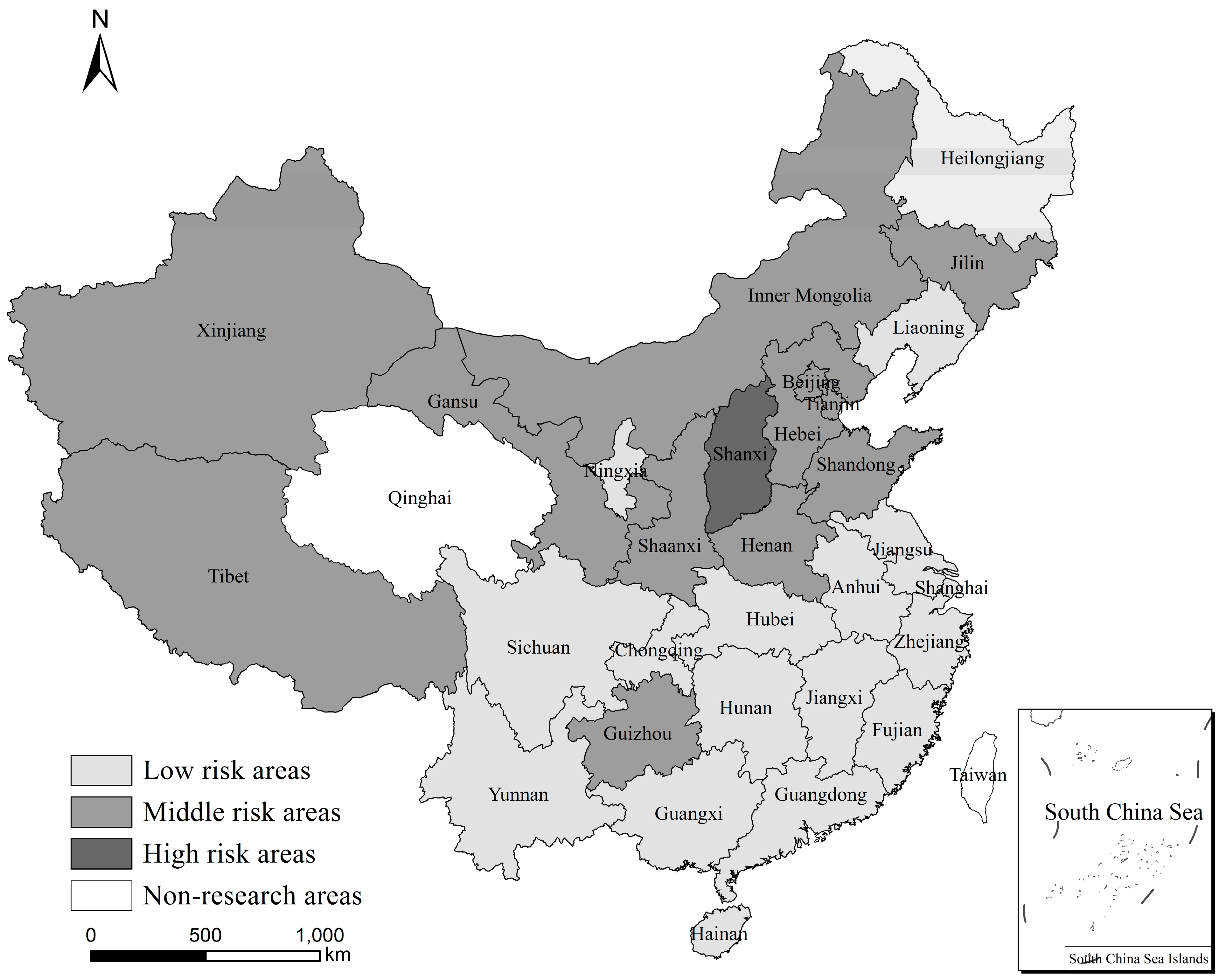
4.2.1. Risk Zone

Through the analysis on the stability, comprehensive comparative advantages and risk probability of rice production in China, generally the national rice yield was more stable, and it had a smaller probability to have a yield loss rate greater than 5%. However, for the 30 provinces, there were significant differences in the stability, integrated comparison advantage of the rice production and the highest yield loss rate of the disaster risk. Therefore, we used the yield loss rate, which is over 5%, as the probability index to assess rice production risk with full consideration of the national and provincial ultra-probability.

At the same time, we have tested three implied assumptions, that is the relations between C.V., comprehensive superiority index, risk probability and risk level. The relations could be interpreted as follows: First, C.V. was directly proportional to the risk level. This meant that the production risk would be changed according to the changes of C.V. Second, the comprehensive superiority index and risk level were inversely related. This showed that the rice production risk would be high or low when the comprehensive comparative advantage became weaker or stronger based on the relative changes in the index. Third, the risk probability and risk level were proportional. This implied that the risk level would change based on the changes in the probability value and the highest yield loss rate.

In order to analyze further the differences of provinces and to cluster the risk level, we chose C.V., the comprehensive comparative advantage and risk probability as the clustering index. Accordingly, with the relative cluster analysis theory [36,37] and software (SPSS17.0), we divided the rice production risk into three (high, middle and low) risk zones in the 30 provinces. As shown in Table 4, the high risk zone included just one province, Shanxi; the intermediate risk area consisted of 12 provinces; and the low risk region included 17 provinces. What is more, the detailed risk zone is shown in Figure 3.

Shanxi, as the only high risk province (its C.V. was 0.3158), reached the highest value among the 30 provinces. This meant that its rice yield had high volatility. Its comprehensive comparative advantage was also not significant according to its comprehensive comparative advantage index. It reached 0.0483 and became the lowest level in the whole country. Its risk probability was 0.3473, which meant that there would be a disaster risk of rice production with a yield loss rate over 5% one time every 3 years. This was much higher than other provinces’ frequencies.

Table 4. Disaster risk zone of rice production in China.

Risk Level		Province	C.V.	Comprehensive Index	Risk Probability (Yield Loss Rate > 5%)
Low	low	Shanghai	0.0341	1.3896	0.0023
		Jiangsu	0.0356	1.3862	0.0014
		Guangdong	0.0369	1.4242	0.0004
		Hubei	0.0339	1.3084	0.0000
		Guangxi	0.0395	1.2639	0.0208
		Zhejiang	0.0516	1.4753	0.0095
		Fujian	0.0594	1.3662	0.0000
		Jiangxi	0.0521	1.6341	0.0000
		Hunan	0.0234	1.5898	0.0000
	middle	Heilongjiang	0.0543	1.0267	0.0577
		Yunnan	0.0662	0.9241	0.0773
		Anhui	0.0699	1.0997	0.0993
		Hainan	0.0704	1.1975	0.0987
		Sichuan	0.0506	1.1510	0.0809
		Liaoning	0.0570	0.9780	0.1437
	high	Chongqing	0.1043	1.1105	0.1674
		Ningxia	0.0317	0.6750	0.0011
average			0.0512	1.2353	0.0447
Middle	low	Tianjin	0.1418	0.4400	0.2188
		Henan	0.1357	0.4811	0.2190
		Xinjiang	0.1413	0.3360	0.2617
		Jilin	0.1601	0.8947	0.2468
		Guizhou	0.1168	0.8774	0.2243
	middle	Inner Mongolia	0.1123	0.2905	0.1028
		Tibet	0.1204	0.1438	0.0801
		Gansu	0.1143	0.1018	0.1223
		Shandong	0.1088	0.2850	0.0544
		Hebei	0.1418	0.2288	0.1389
	high	Beijing	0.0420	0.1976	0.0627
		Shaanxi	0.0732	0.4120	0.1097
average			0.1174	0.3907	0.1535
High		Shanxi	0.3158	0.0483	0.3474

Note: the values of table cells of zero are due to the great number of decimal digits and the limited cell space, but in fact, their real values are not zero.

Table 4. Disaster risk zone of rice production in China.

Risk Level		Province	C.V.	Comprehensive Index	Risk Probability (Yield Loss Rate > 5%)
Low	low	Shanghai	0.0341	1.3896	0.0023
		Jiangsu	0.0356	1.3862	0.0014
		Guangdong	0.0369	1.4242	0.0004
		Hubei	0.0339	1.3084	0.0000
		Guangxi	0.0395	1.2639	0.0208
		Zhejiang	0.0516	1.4753	0.0095
		Fujian	0.0594	1.3662	0.0000
		Jiangxi	0.0521	1.6341	0.0000
		Hunan	0.0234	1.5898	0.0000
	middle	Heilongjiang	0.0543	1.0267	0.0577
		Yunnan	0.0662	0.9241	0.0773
		Anhui	0.0699	1.0997	0.0993
		Hainan	0.0704	1.1975	0.0987
		Sichuan	0.0506	1.1510	0.0809
		Liaoning	0.0570	0.9780	0.1437
	high	Chongqing	0.1043	1.1105	0.1674
		Ningxia	0.0317	0.6750	0.0011
average			0.0512	1.2353	0.0447
Middle	low	Tianjin	0.1418	0.4400	0.2188
		Henan	0.1357	0.4811	0.2190
		Xinjiang	0.1413	0.3360	0.2617
		Jilin	0.1601	0.8947	0.2468
		Guizhou	0.1168	0.8774	0.2243
	middle	Inner Mongolia	0.1123	0.2905	0.1028
		Tibet	0.1204	0.1438	0.0801
		Gansu	0.1143	0.1018	0.1223
		Shandong	0.1088	0.2850	0.0544
		Hebei	0.1418	0.2288	0.1389
	high	Beijing	0.0420	0.1976	0.0627
		Shaanxi	0.0732	0.4120	0.1097
average			0.1174	0.3907	0.1535
High		Shanxi	0.3158	0.0483	0.3474

Note: the values of table cells of zero are due to the great number of decimal digits and the limited cell space, but in fact, their real values are not zero.

Compared to the corresponding indicators of Shanxi, the C.V. and risk probability reduced significantly and the comprehensive comparative advantage index increased substantially in the middle risk zone. Their averages of C.V., comprehensive comparative advantage indexes and risk probabilities were 0.1174, 0.3907 and 0.1535, respectively. We could get 3 groups as subdividing the middle risk area. The first group included Tianjin, Henan, Xinjiang, Jilin and Guizhou. The C.V., comprehensive superiority index and risk probability were higher and reached 0.1391, 0.6058 and 0.2341, respectively. Although the comprehensive superiority in this group was quite higher, its production volatility and risk were great, so that it was categorized as a middle-high risk area. The second group consisted of Inner Mongolia, Tibet, Gansu, Shandong and Hebei. The relative index averages were 0.1195, 0.2100 and 0.09973. Compared to the first group, the frequency stability of rice production had increased but the risk greatly reduced, and the comprehensive superiority advantage was quite lower, so that it was categorized as a middle-middle risk area. The values of the indicators were 0.0576, 0.3048 and 0.0862 in the third group. This included Beijing and Shaanxi. Its stability and comprehensive advantage of rice production were much better. Although the comprehensive superiority index had improved, the absolute value was still small, so that it categorized as a middle-low risk area.

Figure 3. Disaster risk zone of rice production in every risk area.

Figure 3. Disaster risk zone of rice production in every risk area.

The low risk area consisted of 17 provinces. Their C.V., comprehensive strength index and risk probability were 0.0512, 1.2353 and 0.0447, respectively. In contrast to the middle risk area, rice production stability has increased and the disaster risk has reduced due to the reduction in C.V. and risk probability in the low risk areas. The rice production in those areas had significant comprehensive advantage due to the increase in the comprehensive strength index, which was greater than 1. Similar to the classification in the intermediate risk area, we also divided this area into 3 groups. The first group was comprised of Chongqing and Ningxia, called the low-high risk area, whose corresponding indicators were followed by 0.0680, 0.8928 and 0.0843. The second group was called the low-middle risk area and included Heilongjiang, Yunnan, Anhui, Hainan, Sichuan and Liaoning. Their corresponding indicators were followed by 0.0614, 1.0628 and 0.0929. The third one, called the low-low risk area, consisted of Shanghai, Jiangsu, Guangdong, Hubei, Guangxi, Fujian, Jiangxi, Hunan and Zhejiang, whose corresponding indexes were 0.0407, 1.4264 and 0.0069.

4.2.2. Economic Loss Scenario Analysis

Assuming that the external environment of economic events will not change or only a little, traditional quantitative prediction methods used past system rules or present financial events to assess future trends. These methods ignored the influence of the economic environment and other external factors. Scenario analysis is a combination of qualitative and quantitative forecasting methods, taking full account of the external economic environment factors. It provides a detailed analysis of the development of events influenced by various factors.

In this study, according to the risk probability index of national rice production, we divided the rice yield loss rates into 5 kinds—5%, 10%, 30%,70% and 100%—when measuring the risk of the economic loss of the national rice production. Combined with the accounting methods of stricken, disaster and total crops failure areas given by national water conservancy bureau agriculture ministry and in conjunction with the formula of relevant scholars [32]:

$$R{\text{=A}}_Y·D_S·L$$

(19)

and:

$$E=1.2R$$

(20)

We calculated the rice loss $R$ and economic loss $E$. In Formula (19), ${\text{A}}_Y$, $D_S$ and $L$, respectively, mean yield per unit area, disaster area and loss rate of rice production. As mentioned above, L meat the scenario loss rate of rice production in the national level. The variation R means the min purchasing price of rice in 2012 in China (0.2 dollars/kg). The mean of national rice yield was 6843.78 kg·hm⁻² from 2000 to 2012. The average agricultural disaster was about 24.60 million hectares, and the proportion of rice cultivated to the total crops was 19.92% since reform and opening. So we used this to measure the rice disaster area. The concrete results are shown in Table 5.

The disaster areas of rice production could not exceed cultivated areas, so we took 19.92% as the max proportion of the disaster area and then reduced the proportion by Step 1. Because of the similar theory, we only listed some proportions and the relative disaster areas. Combining the data in Table 5, we calculated that the max yield loss of rice production was 33.53 million tons, and the corresponding economic loss was about 6.71 million dollars. The min yield loss of rice production was 1.68 million tons, and the respective economic loss was about 0.34 million dollars at the different disaster loss rates when the proportion of the disaster area was 19.92%. Similarly, we could obtain other yield loss and the corresponding economic loss of rice production at different disaster loss rates and proportions.

Table 5. The yield and economic loss of rice production in China.

Disaster Proportion		19.92%	18.00%	17.00%	15.00%	10.00%	5.00%
Disaster Areas/hm2		4,899,847.43	4,428,035.54	4,182,033.57	3,690,029.62	2,460,019.75	1,230,009.87
yield loss	5%	1,676,672.67	1,515,223.95	1,431,044.84	1,262,686.62	841,791.08	420,895.54
	10%	3,353,345.33	3,030,447.89	2,862,089.68	2,525,373.25	1,683,582.16	841,791.08
	30%	10,060,036.00	9,091,343.68	8,586,269.03	7,576,119.74	5,050,746.49	2,525,373.25
	70%	23,473,417.33	21,213,135.26	20,034,627.75	17,677,612.72	11,785,075.15	5,892,537.57
	100%	33,533,453.34	30,304,478.95	28,620,896.78	25,253,732.46	16,835,821.64	8,417,910.82
maximum yield loss/t		33,533,453.34	30,304,478.95	28,620,896.78	25,253,732.46	16,835,821.64	8,417,910.82
minimum yield loss/t		1,676,672.67	1,515,223.95	1,431,044.84	1,262,686.62	841,791.08	420,895.54
maximum economic loss/dollar		6,706,690.67	6,060,895.79	5,724,179.36	5,050,746.49	3,367,164.33	1,683,582.16
minimum economic loss/dollar		335,334.53	303,044.79	286,208.97	252,537.33	168,358.22	84,179.11

Table 5. The yield and economic loss of rice production in China.

Disaster Proportion		19.92%	18.00%	17.00%	15.00%	10.00%	5.00%
Disaster Areas/hm2		4,899,847.43	4,428,035.54	4,182,033.57	3,690,029.62	2,460,019.75	1,230,009.87
yield loss	5%	1,676,672.67	1,515,223.95	1,431,044.84	1,262,686.62	841,791.08	420,895.54
	10%	3,353,345.33	3,030,447.89	2,862,089.68	2,525,373.25	1,683,582.16	841,791.08
	30%	10,060,036.00	9,091,343.68	8,586,269.03	7,576,119.74	5,050,746.49	2,525,373.25
	70%	23,473,417.33	21,213,135.26	20,034,627.75	17,677,612.72	11,785,075.15	5,892,537.57
	100%	33,533,453.34	30,304,478.95	28,620,896.78	25,253,732.46	16,835,821.64	8,417,910.82
maximum yield loss/t		33,533,453.34	30,304,478.95	28,620,896.78	25,253,732.46	16,835,821.64	8,417,910.82
minimum yield loss/t		1,676,672.67	1,515,223.95	1,431,044.84	1,262,686.62	841,791.08	420,895.54
maximum economic loss/dollar		6,706,690.67	6,060,895.79	5,724,179.36	5,050,746.49	3,367,164.33	1,683,582.16
minimum economic loss/dollar		335,334.53	303,044.79	286,208.97	252,537.33	168,358.22	84,179.11

In addition, we also found that the rice yield and economic loss would become large (small) according to the increasing (reducing) of the disaster risk loss rate under the same disaster area. However, relative to the same disaster loss rate, the yield and economic loss would be low (high) as the disaster proportion reduces (increases). For the proportions and risk rates in all of the research disaster area, the max national yield loss was 33.54 million tons, and the corresponding economic loss was 6.71 million dollars when the disaster area was 19.92% and the risk loss was 100%. The min yield loss was 420,900 tons, and relative economic loss was 84,179.11 dollars when the disaster area proportion and risk loss rate were both 5%.

5. Discussion and Conclusions

5.1. Discussion

Based on the data of rice production in China form 2000 to 2012, we analyzed the stability and comparative advantage of rice production in 30 provinces. Then, we used the non-parametric information diffusion model based on entropy theory to assess the rice disaster risk. The risk level were divided according to the hierarchical cluster analysis into three indexes, such as C.V., comprehensive efficiency index and risk probability (yield loss rate >5%). Finally, we used scenario analysis to assess the economic loss of national rice production risk.

From the analysis, we found that: First, on the whole, the rice yield in China had a higher stability with a C.V. of 0.0345. However, there were clear differences in provinces’ rice stability. For example, as the main rice production regions in China, Hubei, Hunan, Shanghai and Ningxia Hui autonomous region had a quite stable cultivated area and total output of rice production. Therefore, they had better rice stability. However, for other provinces, the rice production stability was not significant, due to the fluctuations and the differences of rice cultivated area and total output.

Second, from the perspective of the comprehensive advantage index, there were obvious differences between the provinces. Fourteen provinces had significant comprehensive comparative advantages with the index over one. The rest did not have this advantage, due to a lack of efficiency or scale advantage.

Third, the national rice production risk was quite lower with a yield loss rate less than 5%. However, there were more differences between provinces. The yield loss rates in provinces were much higher than the national level, except four provinces: Hunan, Fujian, Jiangxi and Hubei.

Fourth, from the results of the risk zone, there were one province, Shanxi, in the high risk area; 12 provinces belonged to the middle risk; and the rest of the 17 provinces were in the main rice production regions in the low risk area.

Fifth, the yield and economic loss of rice production were directly proportional to the disaster areas and loss rates through measuring the economic loss.

In addition, during this research, as for some specific data, we used an indirect means to measure the economic loss. We obtained some research data according to the converting of rice, crop cultivated areas and crop disaster areas. Therefore, to a certain extent, there were some errors when we were calculating the max or min yield and economic loss under the given disaster area and loss rate. As a result, we need to collect more data and find innovative ways to calculate economic loss in a future study. What is more, although without considering the calculation error, the economic loss estimation objects were the national rice production risk, not every divided risk zone. Therefore, we will refine and subdivide the object of economic loss and make a comparison in economic loss between different risks areas in the future study.

5.2. Conclusions

Based on the above analyses, we could obtain some results by assessing the risk and measuring the economic loss of rice production in China. Accordingly, the interpretation of the results is that the low risk area of rice production in China mainly belonged to two areas, southern and central China, which was inconsistent with the findings of previous scholars [27]. The reasons can be explained as follows: First, we used the C.V., comprehensive advantage index and risk probability as the risk zone index. As for the main rice production provinces, their yield stability was higher than other provinces to some extent. Second, we used the yield loss rate as the basic data to measure the disaster data. In addition, they had significant comprehensive advantages resulting from the natural conditions or advanced AST, which would be superior, and conducive to the growth of rice. Therefore, the yield loss rate in the main production area was quite lower, and most belonged to the low risk zone.

The above research implies the following: Firstly, we should give more attention to AST to increase the rice yield and its stability. From the above analyses, there were big differences in the stability of rice production in research provinces due to the variances of rice yield. At present, the rice yield heavily depends on AST, as the natural constraints increase. As a result, the improvement in the rice yield is more dependent on the investment in AST. What is more, at the same time, we could not ignore the transformation and management of AST in order to improve its application efficiency.

Secondly, optimizing the planting structure would be good for improving the overall production productivity. There were 14 provinces with significant comprehensive advantage, and the others did not, because of the relative lower production, scale level or land output rate based on the deep analysis of the comprehensive comparative advantage. As for the assessment and the zone of the rice risk, some provinces had higher production risk due to a bad natural environment or poor yield stability. Therefore, it is necessary to maximize a specific production advantage according to the local conditions of rice production during the agricultural planting structure layout.

Thirdly, the infrastructure has to be strengthened, and a good disaster prevention mechanism needs to be established. Through the analyses of the production and economic loss, we could draw the conclusion that the absolute loss and economic loss of rice production would increase as the disaster areas and the loss rate increase. It is necessary to continue to improve infrastructure, such as giving more attention to strengthening reservoirs to adjust moisture levels in drought and flood disaster areas and controlling the degree of hazard in a timely manner to reduce the risk loss by managing daily rice production and monitoring or warning of pests and diseases.

References

1. Smallman, C. Challenging to the Orthodoxy in Risk Management. Risk Manag. Soc. 2000, 16, 53–79. [Google Scholar]
2. Aven, T. The Risk Concept—Historical and Recent Development Trends. Reliab. Eng. Syst. Saf. 2011, 99, 33–44. [Google Scholar] [CrossRef]
3. Verbrugge, L.N.H.; van der Velde, G.; Hendriks, A.J.; Verreycken, H.; Leuven, R.S.E.W. Risk Classifications of Aquatic Non-native Species: Application of Contemporary European Assessment Protocols in Different Biogeographically Settings. Aquat. Invasions 2012, 7, 49–58. [Google Scholar] [CrossRef] [Green Version]
4. Slenning, B.D.; Gardner, I.A. Economic Evaluation of Risk to Producers Who Use Milk Residue Testing Programs. J. Am. Veterinary Med. Assoc. 1997, 211, 419–427. [Google Scholar]
5. Burger, J.; Gocheld, M.; Powers, C.W.; Kosson, D.; Clarke, J.; Brown, K. Mercury at Oak Ridge: Outcomes from Risk Evaluations can Differ Depending upon Objectives and Methodologies. J. Risk Res. 2014, 17, 1109–1124. [Google Scholar] [CrossRef]
6. Liao, K.J.; Amar, P.; Tagaris, E.; Russell, A.G. Development of Risk-based Air Quality Management Strategies under Impacts of Climate Change. J. Air Waste Manag. Assoc. 2012, 62, 557–565. [Google Scholar] [CrossRef] [PubMed]
7. Hochman, Z.; Carberry, P.S.; Robertson, M.J.; Gaydon, D.S.; Bell, L.W.; Mclntosh, P.C. Prospects for Ecological Intensification of Australian Agriculture. Eur. J. Agron. 2014, 44, 109–123. [Google Scholar] [CrossRef]
8. Kagabo, D.M.; Stroosnijder, L.; Visser, S.M.; Moore, D. Soil Erosion, Soil Fertility and Crop Yield on Slow-forming Terraces in the Highlands of Buberuka, Rwanda. Soil Tillage Res. 2013, 128, 23–29. [Google Scholar] [CrossRef]
9. Miller, W.W.; Ching, C.T.K.; Yanagida, J.F.; Moore, D. Agricultural Water Pollution Control: An Interdisciplinary Approach. Environ. Manag. 1985, 9, 1–6. [Google Scholar] [CrossRef]
10. Rizzardini, C.B.; Goi, D. Sustainability of Domestic Sewage Sludge Disposal. Sustainability 2014, 6, 2424–2434. [Google Scholar] [CrossRef]
11. Charles, M.B.; Brain, P.B. Perspective on Dietary Risk Assessment of Pesticide Residues in Organic Food. Sustainability 2014, 6, 3552–3570. [Google Scholar] [CrossRef]
12. Ghaida, T.A.; Spinnler, H.E.; Soyeux, Y.; Hamieh, T.; Medawat, S. Risk-based Food Safety and Quality Governance at the International Law, EU, USA, Canada and France: Effective System for Lebanon as for the WTO Accession. Food Control 2014, 44, 267–282. [Google Scholar] [CrossRef]
13. Alawa, D.A.; Asogwa, V.C.; Ikelusi, C.O. Measures for Mitigating the Effects of Climate Change on Crop Production in Nigeria. Am. J. Clim. Chang. 2014, 3, 161–168. [Google Scholar] [CrossRef]
14. Jaime, A.; Ana, R.G.; Irina, O. Principles for the Risk Assessment of Genetically Modified Microorganisms and Their Food Products in the European Union. Int. J. Food Microbiol. 2013, 167, 2–7. [Google Scholar] [CrossRef] [PubMed]
15. Justin, T.; Kristine, M.G.; Robert, P.B. Testing the Environmental Kuznets Curve Hypothesis for Biodiversity Risk in the US: A Spatial Econometric Approach. Sustainability 2011, 3, 2182–2199. [Google Scholar] [CrossRef]
16. Lin, J.; Chen, J.J.; Wang, J.Y.; Li, L.C.; Ma, Z.G.; Yang, K.; Xu, Z.H. Frost Disaster Risk Assessment of Crop in Fujian Province Based on Information Diffusion Theory. Chin. J. Agro-Meteorol. 2011, 32, 188–191. (In Chinese) [Google Scholar]
17. Bordi, I.; Fraedrich, K.; Petitta, M. Large-scale Assessment of Drought Variability Based on NCEP/NCAR and ERA-40 Reanalyzes. Water Resour. Manag. 2006, 20, 899–915. [Google Scholar] [CrossRef]
18. Huang, M.L.; Zhao, K.J. A Weighted Estimation for Risk Model. ISRN Probab. Stat. 2013, 2013, 1–12. [Google Scholar]
19. Kaoru, T.; Masato, S. Quantitative Risk Assessment for Future Meteorological disasters. Clim. Chang. 2012, 113, 867–882. [Google Scholar] [CrossRef]
20. Hansson, K.; Larsson, A.; Danielson, M.; Ekenberg, L. Coping with Complex Environmental and Societal Flood Risk Management Decision: An Integrated Multi-criteria Framework. Sustainability 2011, 3, 1357–1380. [Google Scholar] [CrossRef]
21. Craig, W.T.; Joel, K.S.; Sergei, A.F. Managing Typhoon Related Crop Risk at WPC. Agric. Agric. Sci. Procedia 2010, 1, 204–211. [Google Scholar] [CrossRef]
22. Flowerdew, J.; Horsburgh, K.; Wilson, C.; Mylne, K. Development and Evaluation of an Ensemble Forecasting System for Coastal Storm Surges. Q. J. R. Meteorol. Soc. 2010, 136, 1444–1456. [Google Scholar] [CrossRef]
23. Tariq, M. Risk-based Flood Zoning Employing Expected Annual Damages: The Chenab River Case Study. Stoch. Environ. Res. Risk Assess. 2013, 27, 1957–1966. [Google Scholar] [CrossRef]
24. Huang, X.M.; Wang, L.L. Conditions of Agricultural Catastrophe Risks in China and Establishment of Agricultural Risks Protection Systems. Asian Agric. Res. 2010, 2, 1–3. [Google Scholar]
25. Laura, G. Risk in Agriculture and Opportunities of Their Integrated Evaluation. Procedia-Soc. Behav. Sci. 2012, 62, 783–790. [Google Scholar] [CrossRef]
26. Ozcan, A.U.; Erpul, G.; Mustafa, B.; Erdogan, H.E. Use of USLE/GIS technology integrated with geostatistics to assess soil erosion risk in different land uses of Indagi Mountain Pass—Çankırı, Turkey. Environ. Geol. 2008, 53, 1731–1741. [Google Scholar] [CrossRef]
27. Xing, L.; Zhong, F.N. Zoning Research and Crop Production. J. Agric. Econ. 2006, 31, 14–16. (In Chinese) [Google Scholar]
28. Cao, W.; Zhong, F.N. Assessment of Economic Loss of Extreme Ice/Snow Disasters Based on CGE Model. J. Nat. Disasters 2012, 21, 191–196. (In Chinese) [Google Scholar]
29. Zhang, P.; Zhong, F.N. Assessment of Regional Flood Disaster Indirect Economic Loss Based on Input-output Model. Resour. Environ. Yangtze Basin 2012, 21, 773–779. (In Chinese) [Google Scholar]
30. Yousra, T.; Jeffrey, K.; Lgor, L. Scenario Analysis: A Review of Methods and Applications for Engineering and Environmental Systems. Environ. Syst. Decis. 2013, 33, 3–20. [Google Scholar] [CrossRef]
31. China National Statistics Bureau. China Statistics Yearbook; China Statistics Press: Beijing, China, 2013.
32. Huang, C.F. Natural Disaster Risk Assessment Theory and Practice; Science Press: Beijing, China, 2005; pp. 76–94. (In Chinese) [Google Scholar]
33. Claude, E.S. A Mathematical Theory of Communication. Bell Syst. Tech. J. 1948, 27, 379–423. [Google Scholar] [CrossRef]
34. Chen, Q.Q.; Li, J.; Liang, B.S. Trend Prediction and Factors Analysis on Grain Yield per unit area of Henan Province. J. Henan Agric. Univ. 2012, 46, 219–222. (In Chinese) [Google Scholar]
35. Oltedal, S.; Rundmo, T. Using Cluster Analysis to Test the Cultural Theory of Risk Perception. Transp. Res. Part F 2006, 10, 254–262. [Google Scholar] [CrossRef]
36. Trebuňa, P.; Halčinová, J. Mathematical Tools of Cluster Analysis. Appl. Math. 2013, 4, 814–816. [Google Scholar] [CrossRef]
37. Li, H.; Yin, H.; Bai, Y.; Wang, Y. Condition Assessment on Risk Loss of Agricultural Flood and Drought Disasters in Hunan Province Based on Information Diffusing Principle. Guangdong Agric. Sci. 2013, 7, 223–226. (In Chinese) [Google Scholar]