1. Introduction
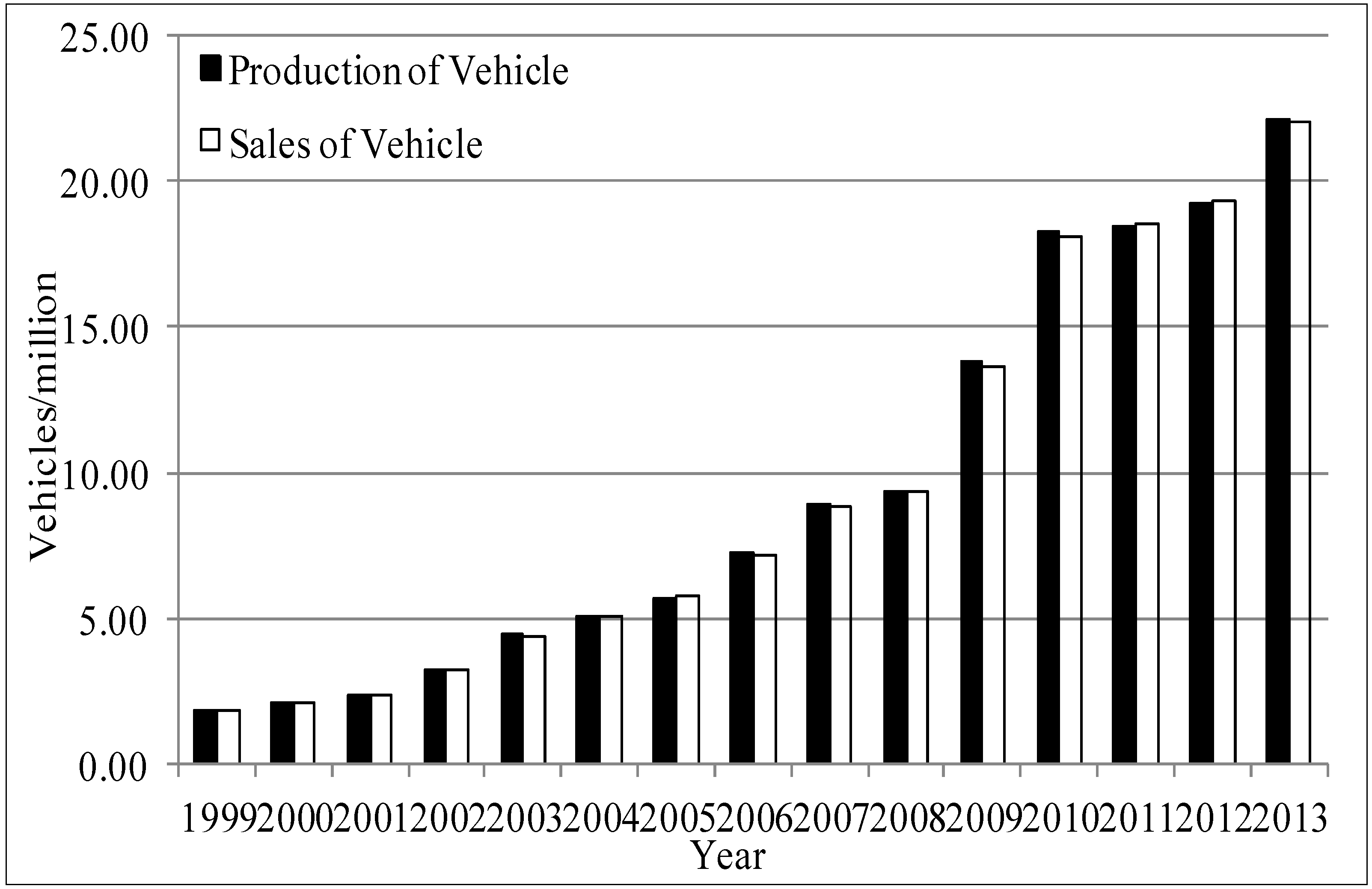
In recent years, the Chinese vehicle fleet has experienced rapid growth (
Figure 1). Data from the China Association of Automobile Manufacturers show that the production and sales of vehicles both exceeded 20 million units in 2013 in China, and that China has been ranked first in the world for production and sales of vehicles for five consecutive years.
Figure 1.
Vehicle production and sales in China, 1992−2013 (Data source: [
1,
2]).
Figure 1.
Vehicle production and sales in China, 1992−2013 (Data source: [
1,
2]).
This result comes with an attendant problem. The increasing energy use and carbon dioxide (CO
2) emissions associated with on-road vehicles are a major challenge in China [
3]. The rapid development of the automotive industry inevitably brings an emission increase. Simonsen and Walnum [
4] showed that its high energy consumption means that transportation accounts for nearly 30% of CO
2 emission in the Organisation for Economic Co-operation and Development (OECD) countries and is one of the main sources of regional and local air pollution. Similarly, He
et al. [
5] estimated that energy use and carbon emissions in the transportation sector will comprise roughly 30% of total Chinese emissions by 2030. There is widespread concern in China at the levels of haze and PM
2.5 (fine particulate matter: up to 2.5 micrometers in size) pollution [
6]. As Lang
et al. [
7] state, a new National Ambient Air Quality Standard (NAAQS) was proposed in China in early 2012, introducing PM
2.5 controls for the first time. Since then, the first thing Chinese residents do each morning is check the Air Pollution Index.
It is therefore necessary to obtain an in-depth understanding of China’s automobile manufacturing developments, particularly in relation to the environmental impacts of Chinese vehicles and to the relationship between vehicle ownership and economic factors. Rather than using per capita income (or per capita disposable income) as an economic factor as previous studies did [
3,
8,
9,
10,
11], we use per capita gross domestic product (GDP) to represent the economic factors. This paper is directly related to Meyer
et al. [
12]. They use the real GDP growth rate of China (Taken from Leimbach and TÒch [
13]) that differ from those mentioned in this paper and develop scenarios for global passenger car stock until 2050. In this paper, we use the GDP index instead of real GDP to do the analysis. The reason is that the GDP index published by China’s National Bureau of Statistics (NBS) is constructed by setting last year’s GDP at 100. Thus, the GDP index can eliminate some effects of inflation on nominal GDP. The real GDP data used in Meyer
et al. [
12] is not available for the public and we cannot find out the reliable real GDP data for China from the current official data source.
Previous studies assumed an annual Chinese GDP growth rate of 6.0%, 4.7%, 4.0%, and 3.0% during each decade from 2011 to 2050 [
14]. Here, we use a multiple autoregressive moving average (MARMA) model to forecast China’s annual GDP growth rate, then undertake the empirical analysis based on this forecast results. The MARMA model is a combination of the regression and autoregressive moving average (ARMA) models. The regression part of the MARMA model can capture the long-term characteristics of the behaviors of GDP growth rate. The ARMA part of the MARMA model can capture the short-term characteristics of the behaviors of GDP growth rate. The tobustness checks and sensitivity analysis for the vehicle stock forecast are subsequently performed to support our research findings.
Our analysis contributes to several literature strands. First, the existing Gompertz curve analyses are successful in specifying features of the vehicle market to explain how to use economic factors to estimate vehicle ownership. Huo and Wang [
3] show that the Gompertz function fits the historical data better than the Logistic or Richards functions. Dargay and Gately [
15] tested several functional forms, and showed that the Gompertz function is somewhat more flexible than the Logistic model, particularly in allowing different curvatures at low- and high-income levels. They also illustrated the characteristics of the Gompertz function for long-run vehicle ownership. Huo
et al. [
14] used the Gompertz function to estimate the 2011–2050 Highway Vehicles (HWVs) stocks in China and projected three vehicle stock scenarios―high-growth, mid-growth and low-growth―by HWV saturation level. Zheng
et al. [
16] used the Gompertz function to calculate county level vehicle ownership and found it to be reliable for simulating city-level vehicle growth patterns in China. However, there are econometric problems in estimating the Gompertz function parameters in these empirical works. A well-known advantage of the Gompertz function is its log-linearization ability [
17]. Thus, previous studies treat it as a linear regression and use Ordinary Least Square (OLS) regression to get the parameters, and focus on the mean value of R-square (R
2) of the linear regression. This ignores the panel data feature. Panel data have two dimensions: time series and cross-section. To apply the usual OLS statistics from the pooled OLS regression across
i and
t, we need to add homoscedasticity and no serial correlation assumptions [
18]. The pooled OLS treat the data as cross sectional and ignores the individual-specific effects [
19]. Zhao [
17] discussed the difference between pooled OLS, Fixed Effects (FE), and the Random Effects (RE), but did not use the Hausman specification test (details in [
20]) to test whether the RE model is resoundingly rejected.
Second, this paper is directly related to Huo and Wang [
3] and Dargay
et al. [
21] for Chinese vehicle stock estimations. Huo and Wang [
3] focus on the country level and estimate Chinese vehicle stocks by the Gompertz, Logistic and Richards functions. They assume two scenarios for the growth of private car ownership in China―a low-growth scenario and a high-growth scenario―where the saturation level of private car ownership per 1000 people is 400 and 500, respectively. Dargay
et al. [
21] found that China has by far the greatest growth in vehicle ownership―10.6% annually―of non-OECD countries. Further, they project that China will have nearly 20 times as many vehicles in 2030 as it had in 2002. This expansion is associated with both China’s rapid income growth and its per capita income during this period being related with vehicle ownership growing at over twice the rate of income. There are several important differences between this paper and those of Huo and Wang [
3] and Dargay
et al. [
21]. First, we use per capita GDP as an economic factor and estimate the annual GDP growth based on the MARMA model regression. Second, we run regression on the Gompertz function by FE and RE, and use the Hausman specification test to confirm the advantage of the FE or RE over a pooled OLS. Third, sensitivity analysis is undertaken, one is that varies the saturation level of vehicle ownership at the same rate of change for each country, and another one is with different GDP growth rate. Fourth, we use a scenario analysis to discuss OECD, Europe, United States (U.S.), and Japan patterns. Finally, we investigate a large sample: 1963–2011 per capita GDP and vehicle ownership in 21 countries and regions.
The remainder of the paper is organized as follows:
Section 2 introduces the methodology and data.
Section 3 presents the empirical model and forecast the annual 2012–2050 vehicle ownership in China.
Section 4 presents the sensitivity analysis and robustness check, and
Section 5 concludes and lays down several implications in terms of sustainability policies.
2. Methodology and Data
In the short term, the variation of supply and price, using cost and consumption policy, may have an impact on vehicle demand and increase short-term fluctuations in the vehicle market. However, in the longer term, vehicle demand shows a highly significant correlation with the level of economic development [
22]. For instance, the Chinese consumption policies differ from the market approach of OECD countries. (1) Bidding to drive: Car License Auction Policy in Shanghai. Shanghai had approximately two million motor vehicles in 2004, increasing to 3.1 million in 2010. As a result, Shanghai has promulgated a vehicle control policy, which uses monthly license auctions to limit the number of new cars [
23]; (2) Beijing’s Vehicle Lottery. Beijing is first and unique in restricting license plates via a random lottery rather than using an auction system. Following Beijing’s lottery and Shanghai’s auction experience, other Chinese cities are considering the similar policies to restrict the vehicle demand and improve the air pollution caused by the high vehicle stock growth [
24].
There are many reasons for relating the vehicle stock to GDP growth in China. At the macro level, with the rapid growth of GDP, labor mobility and capital mobility between different regions should be accelerated. This would cause an obvious increase of the vehicle stock. Also the GDP growth drives the energy consumption up [
25,
26,
27], which gives a chance to increase the vehicle stock for exploring the energy and transferring the energy. At the individual level, for instance, motor vehicles are considered more as necessities than luxury items as income levels transfer from poor to wealthy. Under normal circumstances, strong growth in demand for motor vehicles is consistent with the growth of wealth.
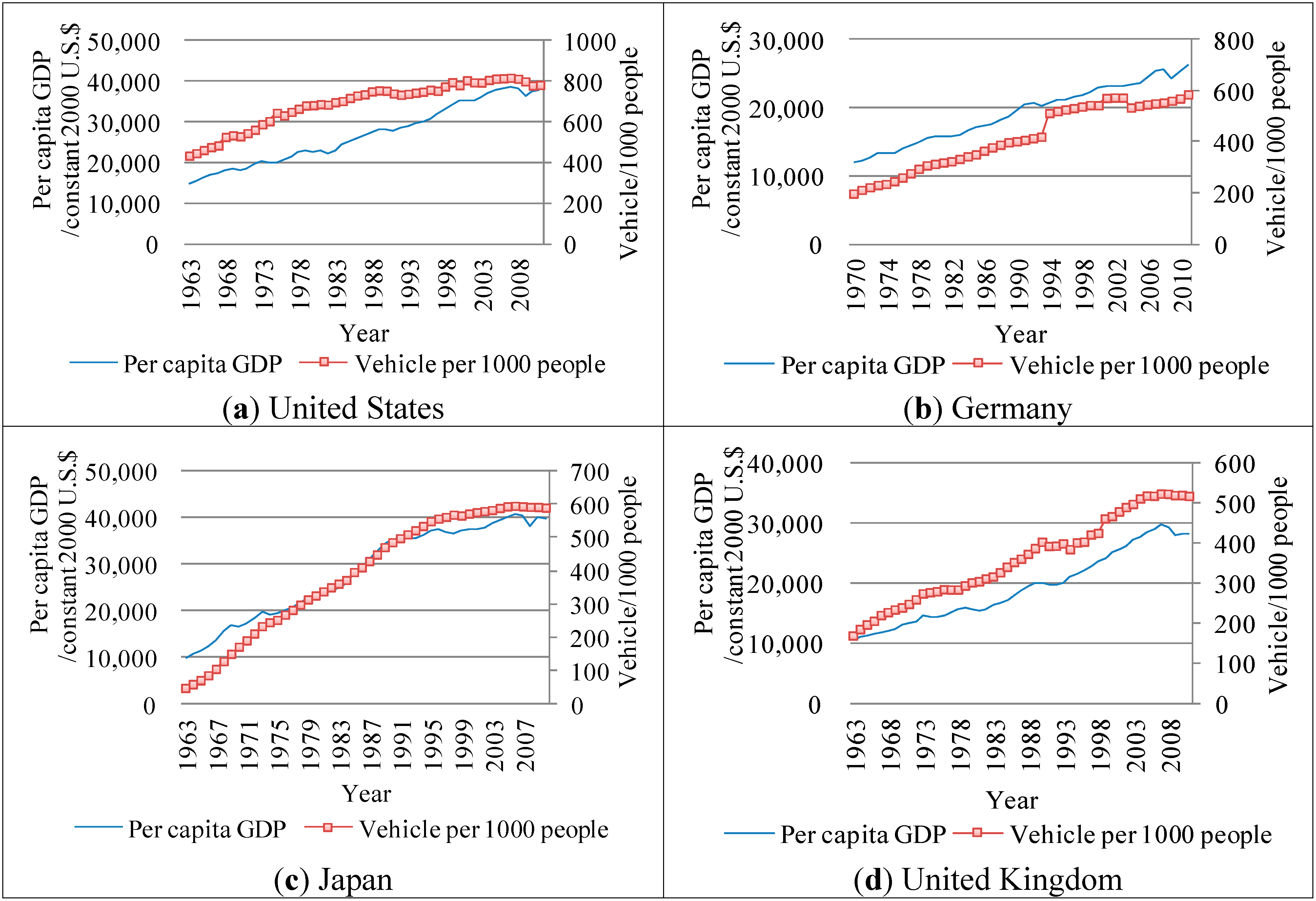
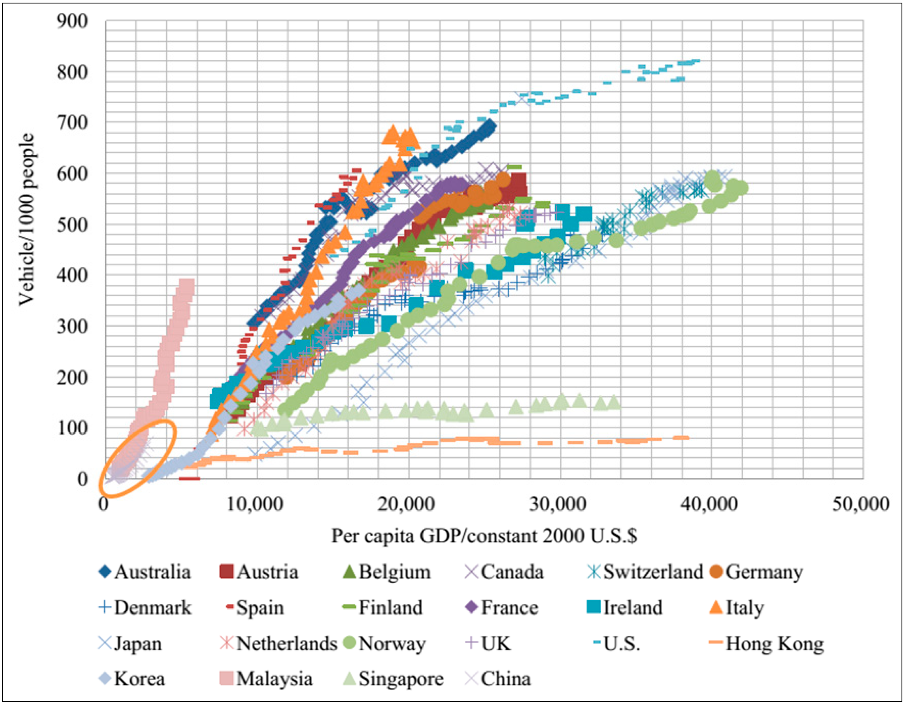
As
Figure 2 shows, there is a highly significant correlation between vehicle ownership per 1000 people and per capita GDP (e.g., U.S., Germany, Japan and the United Kingdom).
Figure 2.
Annual vehicle ownership and economic development (Data source: [
28]).
Figure 2.
Annual vehicle ownership and economic development (Data source: [
28]).
Based on such findings, earlier studies used the historical growth trends in developed countries and employed the S-shaped growth curve [
3,
15,
16,
21,
22]. Zhao [
17] points out that vehicle ownership in most OECD countries has reached the ultimate saturation level and that there is a Gompertz curve function between vehicle stock and GDP per capita; other emerging countries also follow a Gompertz curve pattern and present an upward trend. China is in the primary stage of the Gompertz curve. The Development Research Center of the State Council [
22] provides a theoretical analysis explaining why vehicle demand has an S-shaped growth curve. Without government intervention or vehicle market regulatory policies, vehicle demand changes are influenced by market factors (e.g., consumer income and vehicle price). Vehicle demand clearly increases with a consumer income increase (income effect) or with a vehicle price decrease (price effect). Both conditions may occur simultaneously to give an integrated effect. Historical evidence shows that increasing vehicle demand levels can experience three stages: high-income, middle-income and low-income. Therefore, the vehicle demand growth curve presents a non-linear growth pattern in developed countries that is similar to the S-shape curve (
Figure 3).
In relation to the particularity in China: China’s economic development has two primary characteristics. Firstly, both Chinese GDP and the production and sales of vehicles have experienced tremendous growth in recent years. Secondly, the China’s per capita GDP and vehicle ownership per 1000 people are still well behind advanced countries. As highlighted by Zhao [
17], there is a large population base and the income gap between urban and rural households in China. Thus, we were unable to use Chinese historical data to estimate the Gompertz function. China is still at the start of the Gompertz curve: the orange circle in
Figure 3 (at the lower left corner of the first quadrant) shows China’s current position, close to the origin.
Figure 3.
Worldwide vehicle ownership trends and per capita GDP (Data source: [
28,
29]).
Figure 3.
Worldwide vehicle ownership trends and per capita GDP (Data source: [
28,
29]).
Therefore, this study proceeds as follows. Firstly, we study the vehicle development trends of other developed countries and choose an appropriate data to estimate the key parameters in the Gompertz function. Secondly, we use Chinese GDP historical data to predict the annual 2012–2050 per capita GDP. Finally, we use the parameters estimated in step one and the annual per capita GDP data estimated in step two to predict the annual vehicle ownership in China. This process has an important assumption that the development of China’s vehicle will follow the Gompertz curve path. This assumption is reasonable because (1) vehicle development trends generally follow the Gompertz curve in other countries; and (2) the success of China’s economic development shows that its industry development is imitating the mature experience of other developed countries.
2.1. Economic Factor
The speed of vehicle ownership expansion in developed countries is mainly driven by the demand side of the market; this means that vehicle ownership increases are decided mainly by consumers’ wealth level and purchase intention. The income variable usually better reflects the aggregate demand. Therefore, researchers can use per capita income (or per capita disposable income) as an economic factor in the Gompertz function in developed countries. It is important to note that there are two main differences between China and other developed countries, which lead us to using per capita GDP as an economic factor for China.
First, the statistics relating to Chinese income levels are biased. Microeconometrics has a sizeable volume of literature―statistical deviation―relating to the income levels of Chinese residents. Reported earnings may not fully reflect the actual income of individuals in the state sector, which may result in an underestimation of earnings [
30]. Li and Luo [
31] claim that both disguised subsidies (such as public housing, social insurances) and regional living costs should be considered when estimating income in China.
Second, the balance between vehicle supply and demand is affected by the government’s intervention (e.g., energy efficiency standards, car licensing regulations
etc.) However, the case of China’s vehicle market regulatory policies is much more unique. In recent years, the government introduced several policies to address air pollution and exacerbated congestion. Aside from the aforementioned policies, Car License Auction Policy in Shanghai and Beijing’s Vehicle Lottery, there are some other policies: (1) Odd–Even Day Vehicle Prohibition (OEDVP) where vehicles with odd license plate numbers can only be used on odd days. If the increase of vehicle ownership is decided by consumer wealth and use levels, consumers with high income levels may be incentivized to owning more vehicles under this policy, thus increasing market friction; (2) Other related policies. On 25 February 2014, Xi Jinping, General Secretary of the Communist Party of China’s Central Committee, State President and Chairman of the Central Military Commission, set five development and management requirements, specifically referring to the increasing air pollution control, tackling heavy haze, and improving air quality priorities, including strictly controlling vehicle market sizes [
32].
We use microeconomics to further explain why vehicle ownership is affected by government intervention and regulatory policies: they may dampen consumer behavior. In the view of general equilibrium models of consumers, producers and government, the constraints imposed on consumers by government intervention and regulatory policies is equivalent to restrictions on producers: the government can shift the market distortions to the producers. Therefore, we consider a Government-Producers model, and take the partial equilibrium into account. The vehicle is good with negative externality; it may produce air pollution during its production and use. The government’s objective differs to the firm’s objective. The firm seeks profit maximization, while the Government is concerned with both profit and the negative externality. The government aims for social welfare maximization and reaching the social optimal. Therefore, the optimal investment is IG from the government’s social welfare maximization objective and is IF > IG from the firm’s profit maximization objective. This means that the firm is over-invested in the view of the government. As a result, the government may restrict the production behavior of the firm: this is equivalent to placing restrictions on consumers (e.g., Car License Auction Policy in Shanghai or Beijing’s Vehicle Lottery).
In conclusion, in China, buying a vehicle is not only a self-selection process but also subject to the government intervention and vehicle market regulatory policies. Taking Beijing’s Vehicle Lottery as an example, the difficulty of winning the lottery suggests that many entrants with a high willingness to pay for a vehicle were unable to buy a car [
24]. Affected by such policies, consumers cannot make the decision to buy a vehicle according to their wealth level and purchase intention. We believe that GDP is a typical indicator representing the aggregate economy. It reflects both the aggregate demand and aggregate supply of an economy. The vehicle ownership is not only affected by the demand factor, but also by the supply factor and government intervention and regulatory policies. Therefore, GDP rather than income should be used as the economic factor.
2.2. Gompertz Function
The Gompertz function is widely applied to establish the relationship between vehicle ownership and economic factors [
3,
15,
16,
21]. The Gompertz function is used here to estimate country-level vehicle ownership as follows:
where
i denotes different countries and
t denotes different years;
Vi,t represents the vehicle ownership (vehicles per 1000 people) of country
i in year
t;
Vi* represents the ultimate saturation level of vehicle ownership (vehicles per 1000 people) of country
i. Given the parameters of
α and
β,
Vi,t changes in proportion to the change of
Vi*;
EFi,t represents the economic factor (per capita GDP) of country
i in year
t;
α and
β are two negative parameters that determine the shape of the S-curve. The increase of
α and
β would lead to a steep S-shape curve against the economic factors.
Log-linearization, then Equation (2) is converted from Equation (1)
As shown by Equation (2), ln (−α) and β were linearly related and could be regressed as OLS for time series data in country i.
In this study, we construct a panel data, including data from 1963–2011 within 21 countries and regions. For panel data, based on the books by Baltagi [
33], the Fixed-Effects estimator that amounts to using OLS to estimate Equation (3)
Additionally, the Hausman specification test should be used for clarity in identifying which model (e.g., FE or RE) is the best tool for the Gompertz function.
2.3. Multiple Autoregressive Moving Average (MARMA) Model
We use a MARMA model to forecast China’s GDP growth. The MARMA model is actually an application of the Box-Jenkins methodology. It is the combination of regression model and ARMA model. The regression part captures the long-term characteristics of the behavior of GDP growth and the ARMA part captures the short-term characteristics. The MARMA model is constructed first by running a regression of GDP growth on population growth, and then taking the regression residual. Next, we apply the Box-Jenkins methodology [
34] to the regression residual, then forecast GDP growth up until 2050. The reason for doing this is that the classical growth theory such as the Solow model considers the population as the most important factor affecting the economic growth. To forecast the long-term GDP growth, we would like to control the affected population. Also, as a time series variable, the GDP growth always shows the cyclical moving pattern, which can be described by the ARMA process. Therefore, the MARMA model we use to forecast GDP growth has the following expression:
Define DGDP in Equation (4) as the annual GDP growth rate in period t, which is the dependent variable. μ is the mean of DGDP process. T can be considered to be the time trend. A (L) is the coefficient of lagged DGDP, where L is lag operator and the sum of lagged DGDP is called the autoregressive part of DGDP process. B (L) is the coefficients of disturbance term u and lagged disturbance term, where the sum of disturbance term and lagged disturbance term is called the moving average part of the DGDP process.
2.4. Data
Four sources of data are used in the main empirical work: country-level vehicle ownership data from 1963 to 2011 from the International Road Federation (IRF) world road statistics [
29]; country-level annual GDP data from 1963−2011 from the World Bank open data; country-level annual population data for 1963−2011 from the World Bank open data [
28]; and annual Chinese population prediction data sets for 2012−2050 collected from National Population Development Strategy Research [
35].
Vehicle ownership data includes full vehicles in use for 1963–2011 for different countries. The variables include total vehicles, passenger cars, buses, lorries and vans, and motorcycles. We collected such data for 21 countries and regions, including Australia, Austria, Belgium, Canada, Switzerland, Germany, Denmark, Spain, Finland, France, Ireland, Italy, Japan, Netherlands, United Kingdom, U.S., Republic of Korea, Malaysia, Singapore, China and Hong Kong. The first 17 are OECD countries, and Malaysia, Singapore and Hong Kong are emerging regions.
World Bank open data provided annual GDP and population data. We matched these two datasets with vehicle ownership by year to get a panel data for 1963–2011: this was used in estimating the Gompertz function. Annual GDP data was converted to constant 2000 US$. However, there is a great impact of the China’s reform and opening-up policies on the Chinese economy, and China has pursued sweeping economic changes in an officially sponsored transition. Furthermore, China’s National Bureau of Statistics (NBS) has revised its estimates of nominal GDP from 1978 to 2004 on the basis of nationwide economic censuses in 2004 [
36]. Therefore, we used the the post-1978 data.
National Population Development Strategy Research [
35] provided 38 prediction results of population from 2012 to 2050 in China, which are based on different levels of birth rate, death rate, sex ratio and other factors. Although the annual GDP growth fluctuates, it is a regulatory government economic index. According to the series of reports about the National People’s Congress (NPC) and Chinese People’s Political Consultative Conference (CPPCC) [
37], the annual GDP growth must be stabilized at a suitable level, and the annual GDP growth will be below 8.0% in the long run. The annual population size has an impact on predicting the annual GDP growth when using the MARMA model. The seven results we select are those based on the medium level of birth rate, death rate, sex ratio and other factors. Among these, we choose the average one to do the forecast for GDP growth in the next section and the other six results to do the robustness check. From the above discussion, the independent Gompertz function variable is the economic factor rather than demographic indicators. This implies robust estimation results by using different results of predicting population.
3. Results and Analysis
To estimate the annual 2012–2050 vehicle ownership in China, we need to determine the parameters α, β, and Vi* and the annual per capita GDP in China for the period.
The ultimate saturation level of Chinese vehicle ownership
VChina* was determined through the literature surveys [
3,
14,
16], and we assumed a middle-growth scenario where the saturation level of vehicle ownership per 1000 people is 500. Sensitivity analysis on different ultimate saturation levels of vehicle ownership is undertaken in
Section 4.
For parameters α and β derived from the Gompertz curve, we run regressions based on the OECD (full sample), Europe (including all European countries), U.S., and Japan patterns. The first two samples are panel data that run regressions as in Equation (3); the others are time-series data.
For the annual 2012−2050 Chinese per capita GDP, we use the MARMA model to get the independent variable EFChina,t in the Gompertz function.
The estimations that give us all of the variables are required in estimating the annual vehicle ownership per 1000 people in China by Equation (1).
3.1. Parameters in the Gompertz Function
We use the Hausman specification test to establish whether the FE or the RE model is the best tool to be used in the Gompertz function.
The null hypothesis states that the random effects model is preferable (
Table 1).
Table 1.
Hausman Test in the Gompertz function.
Table 1.
Hausman Test in the Gompertz function.
| | Coefficients |
|---|
| | (b) | (B) | (b−B) | Sqrt (diag(V_b−V_B)) |
| | Fixed | Random | Difference | Standard Error |
| EFi,t | −0.0001382 | −0.0001349 | −3.33×10⁻⁶ | 7.46×10⁻⁷ |
The empirical results are shown in
Table 2. The first two columns show the regression results for the OECD pattern by pooled OLS and FE: the results are significantly different. The middle column shows the European pattern regression results, and the last two columns show the American and Japanese patterns.
Decision: under the current specification, since p-value = 0.0000 < 0.05, reject H0. This means the two models are different enough to resoundingly reject the RE model, and we should choose the FE model.
Table 2.
Regression in the Gompertz function.
We derived the parameters
α,
β from the Gompertz curve (
Table 3).
Table 3.
Parameter estimation in the Gompertz function.
Table 3.
Parameter estimation in the Gompertz function.
| Saturation Level of Vehicle Ownership per 1000 People | α | β |
|---|
| OECD pattern | Saturation level of vehicle ownership for each country | −3.21877 | −0.000138 |
| Europe pattern | Saturation level of vehicle ownership for each country | −3.06792 | −0.000130 |
| U.S. pattern | 800 | −17.8499 | −0.000207 |
| Japan pattern | 590 | −28.3039 | −0.000177 |
Table 3 shows that the absolute value of parameter
α in the U.S. or Japan is larger than those in OECD or European countries; the absolute value of parameter
β shows a similar pattern. There is no significant difference between the absolute value of parameter
α and
β within the OECD and European pattern, because the European sample has dominated (see the last row in
Table 2).
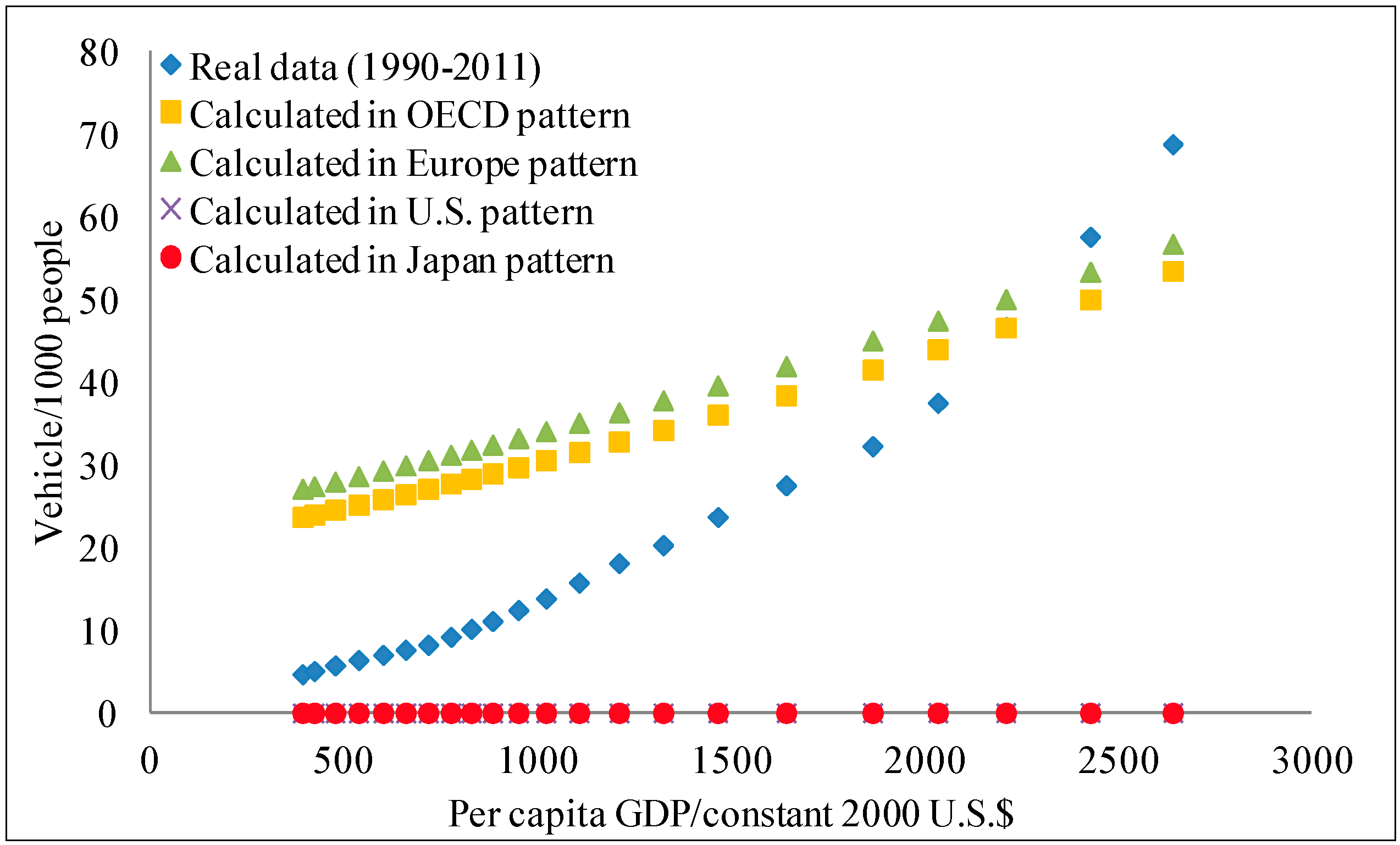
We set the parameter substitution into Chinese data from historical data, comparing real data (
Figure 4).
Figure 4.
Simulated vehicle ownership data in China in different patterns (1990–2011).
Figure 4.
Simulated vehicle ownership data in China in different patterns (1990–2011).
Note: the saturation level of vehicle ownership per 1000 people is 500 in China.
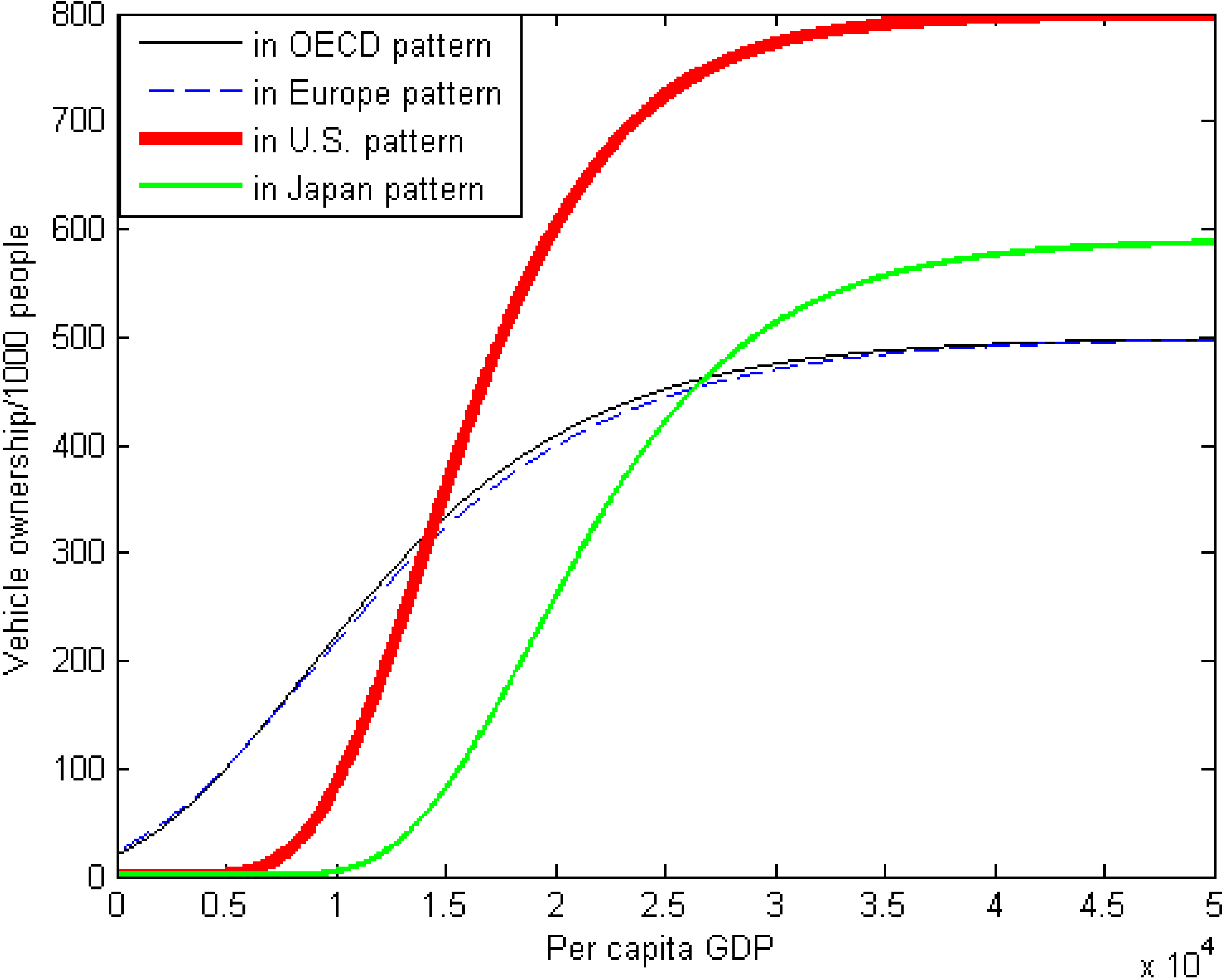
Figure 4 clearly shows that the OECD and Europe patterns fit the real vehicle ownership data best, particularly in the high level of per capita GDP in recent years. In fact, the level of vehicle ownership in the U.S. was 437 per 1000 people in 1963; this approaches the saturation level of vehicle ownership per 1000 people of China. Therefore, we use the parameters
α and
β estimated in the OECD and European patterns to forecast the growth pattern of vehicle ownership in China for 2012−2050. Furthermore, the reason why Japanese and U.S. vehicle ownership patterns are at zero along the different per capita GDP levels shown is due to the large absolute value of parameter α for Japan and U.S., in contrast to a low level of per capita GDP and low level of development of automotive industry for China.
Figure 5 illustrates why the OECD and Europe patterns best fit the real vehicle ownership data of China.
Figure 5.
Simulated vehicle ownership projection to 2050 of China in different patterns.
Figure 5.
Simulated vehicle ownership projection to 2050 of China in different patterns.
Note: Saturation of vehicle ownership per 1000 people is 500 in the OECD and Europe patterns.
In
Figure 5, given per capita GDP, the larger absolute value of parameters
α and
β depict the extremely low value of vehicle ownership per 1000 people in the low level of per capita GDP, with a higher value in the high level of per capita GDP. As mentioned in
Section 2, China is in the primary stage of the Gompertz curve, experiencing tremendous growth in vehicle production and sales and with the Chinese per capita GDP still well behind advanced countries. In the Gompertz curve, the smaller absolute value of parameters α and β best fits the case of lower levels of per capita GDP.
3.2. GDP Growth in China
We built the MARMA model based on the annual GDP growth from 1979 to 2012 (the base period is 1978). We followed Zhao [
17], controlling the annual population growth that may have an impact on the growth of GDP in the channel of the change of labor supply and productivity of labor.
3.2.1. Augmented Dickey–Fuller Unit-Root Test
When the autoregression includes lagged changes, tests for a unit root are described as augmented Dickey–Fuller (ADF) tests [
38].
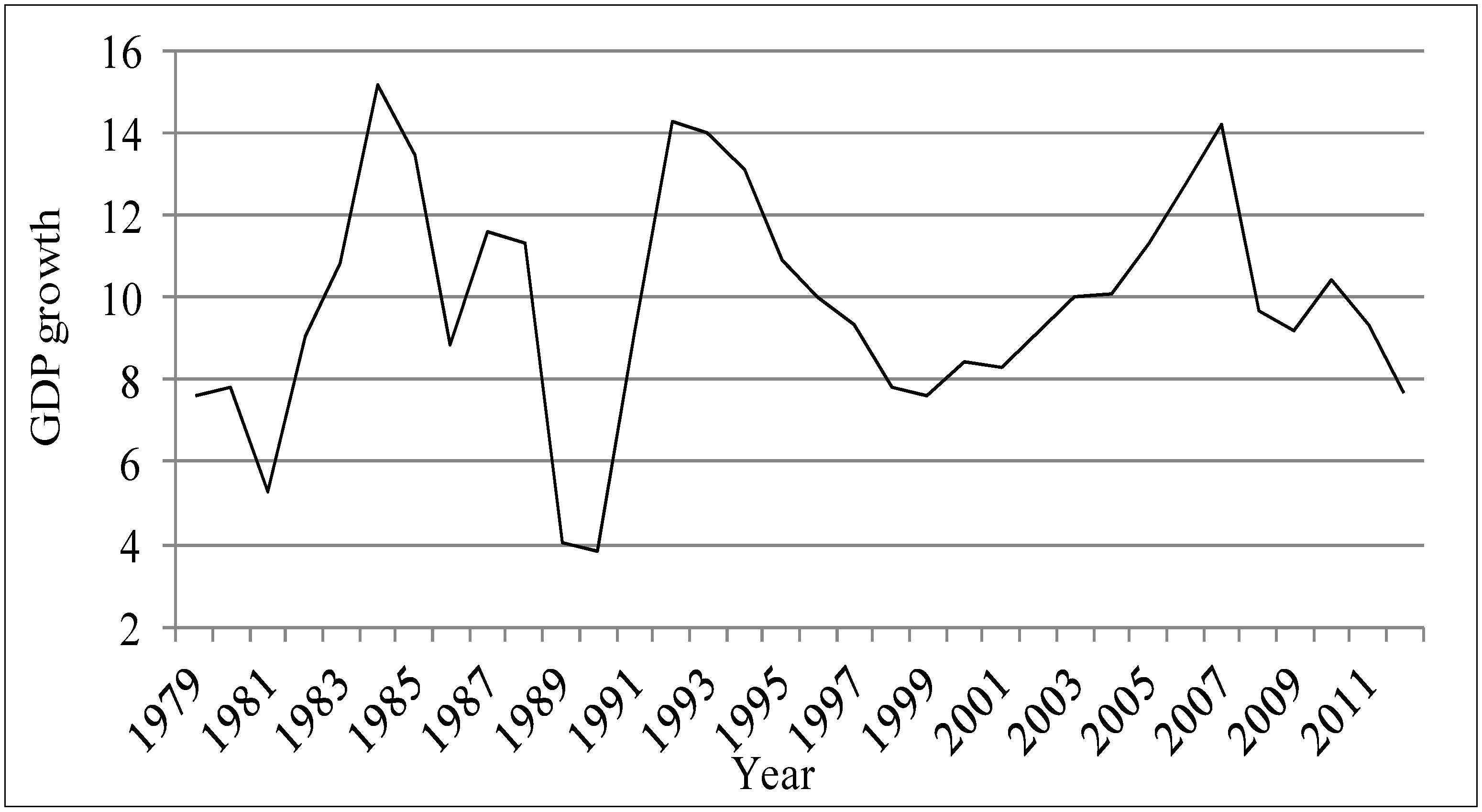
Figure 6 shows the annual GDP growth time series from 1979 to 2012.
Figure 6.
The annual GDP growth (1979−2012) (Data source: [
39]).
Figure 6.
The annual GDP growth (1979−2012) (Data source: [
39]).
The ADF test for the annual GDP growth from 1979 to 2012 shows that the t-statistic for ADF = −4.66 > −2.79 (critical value under the 5% significance level); this rejects H0, and means the annual GDP growth time series is a stationary process. Therefore, we can use these series to build the MARMA model.
3.2.2. Estimation in MARMA Model
According to the analysis by correlation diagram and partial correlation diagram, the order of MARMA process has been determined. Then, we get the estimated function
where
DPOPt is the growth of total population in period
t;
![Sustainability 06 04877 i009]()
is an AR (1) process.
3.2.3. Forecasting the Annual GDP Growth Rate
Based on Equation (6), we can estimate the 2013−2050 annual GDP growth rate.
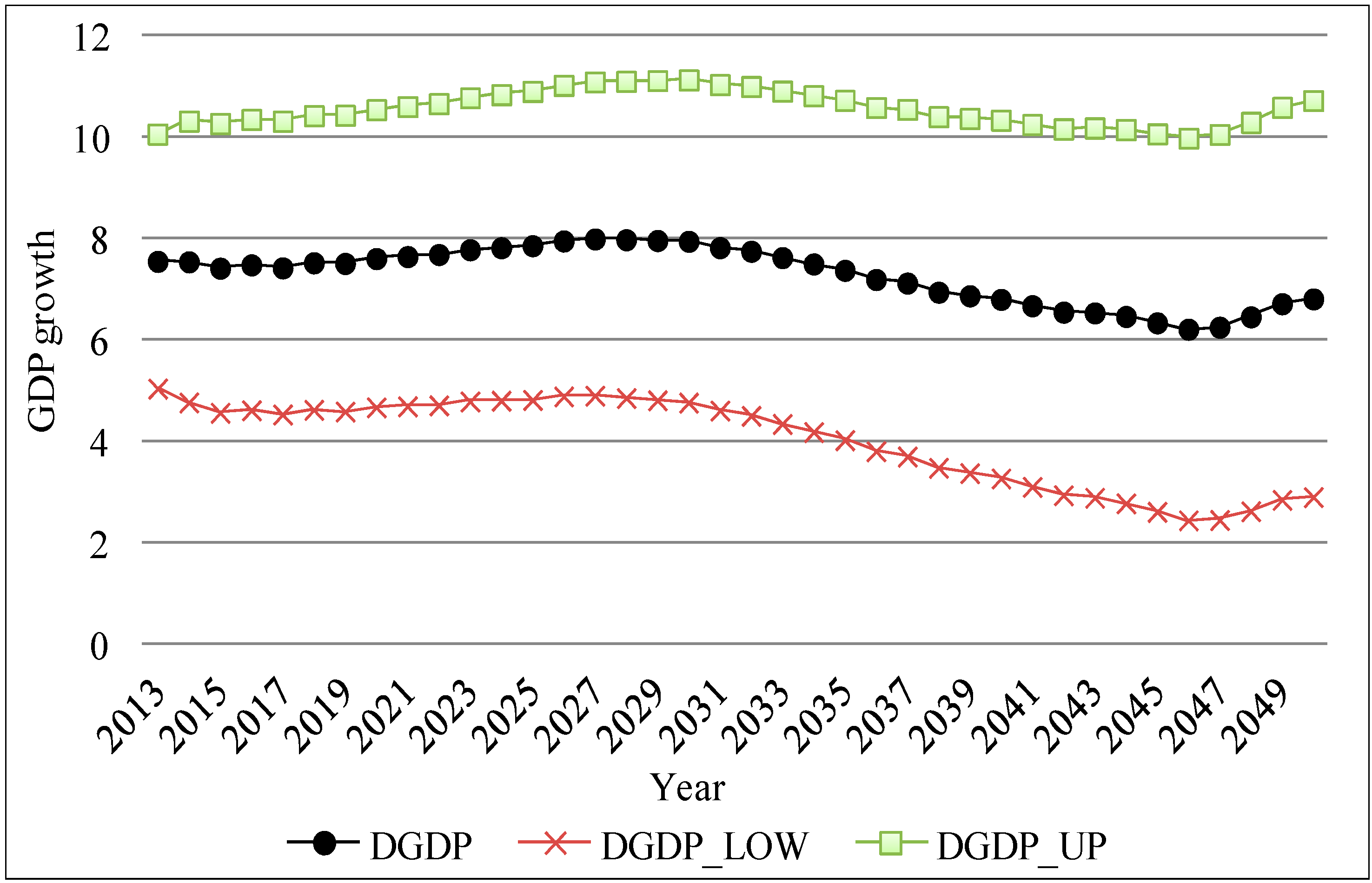
In
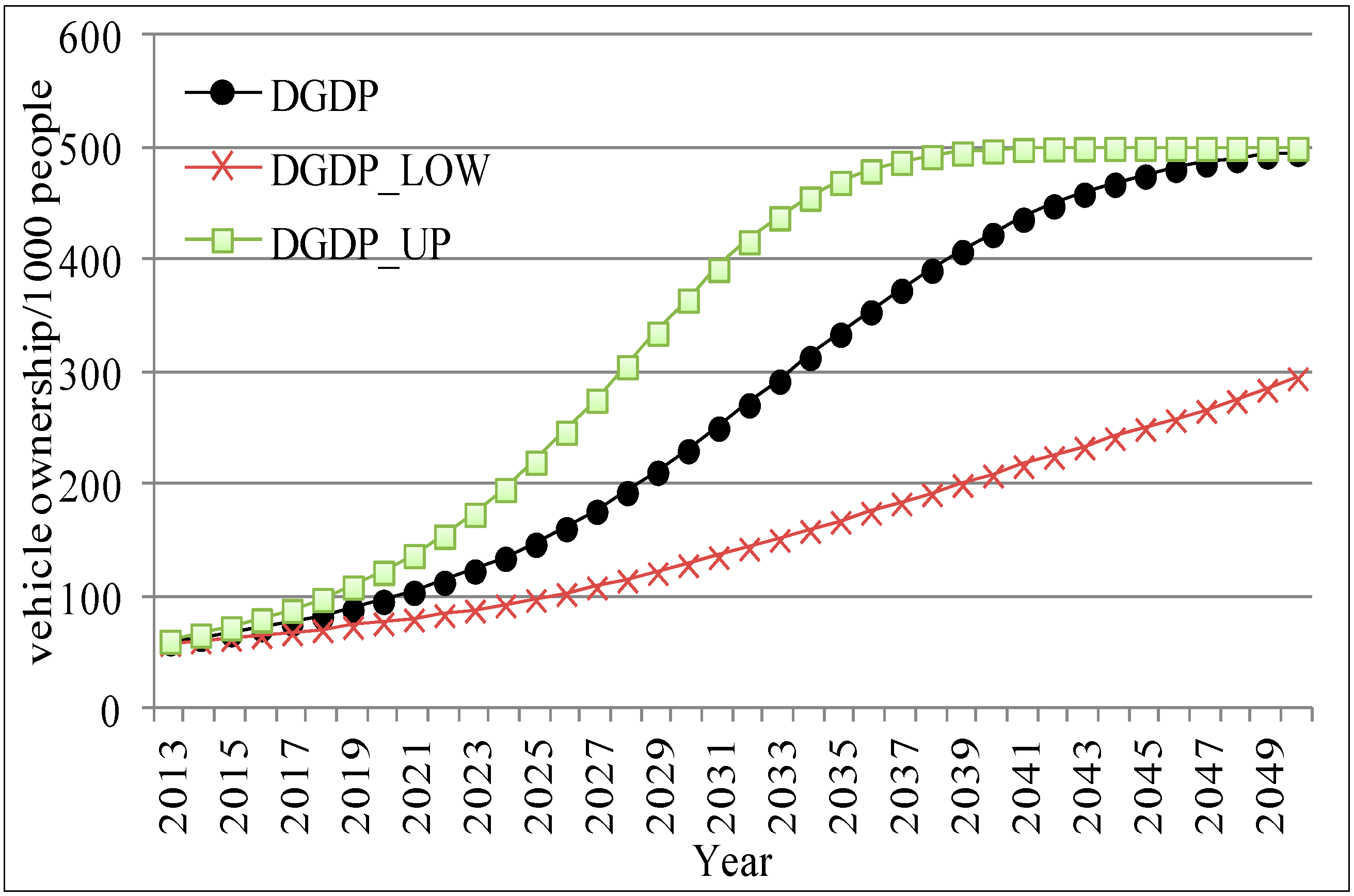
Figure 7, the annual GDP growth is in the moderate range, with a slow growth from 2013 to 2029, then a gradual reduction to nearly 6.0% in 2046 followed by a recovery until 2050. The forecast error bands around the forecasted value are calculated, which shows that the forecasted value stays within the bands with the probability of 68%. Compared with the literature, Huo
et al. [
14] assume China’s annual GDP growth rate to be 6.0%, 4.7%, 4.0%, and 3.0% during each decade from 2011 to 2050. Meyer
et al. [
12] uses real GDP growth rate of China for the analysis, which decreases rapidly from 9% in 2010 to 2% in 2050. Their forecasted values for China’s GDP growth rate lie within the forecast error bands we present here. However, these values are close to the lower band of our results. It must nevertheless be pointed out that the GDP definition varies in different studies. We use the GDP index to do the forecast, resulting in possible discrepancies with other studies. In view of this uncertainty about the forecasted GDP growth rate, we do the sensitivity analysis using different forecasted values of GDP growth in the next section.
Figure 7.
The annual GDP growth rate (2013–2050).
Figure 7.
The annual GDP growth rate (2013–2050).
Note: the DGDP_LOW and DGDP_UP are derived from the DGDP and standard error (S.E).
In period
t, the annual per capita GDP is calculated as
where
POPt is total population in period
t.
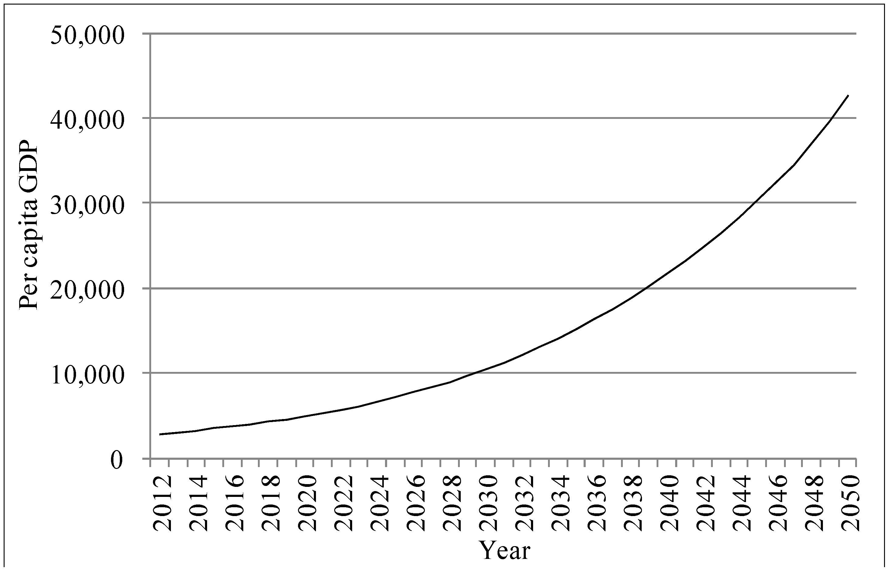
Figure 8 shows the 2013–2050 annual per capita GDP.
Figure 8.
Annual Chinese per capita GDP (2013–2050).
Figure 8.
Annual Chinese per capita GDP (2013–2050).
3.3. Vehicle Ownership Projection in China
All parameters needed for the Gompertz function are now estimated, including the parameters
α and
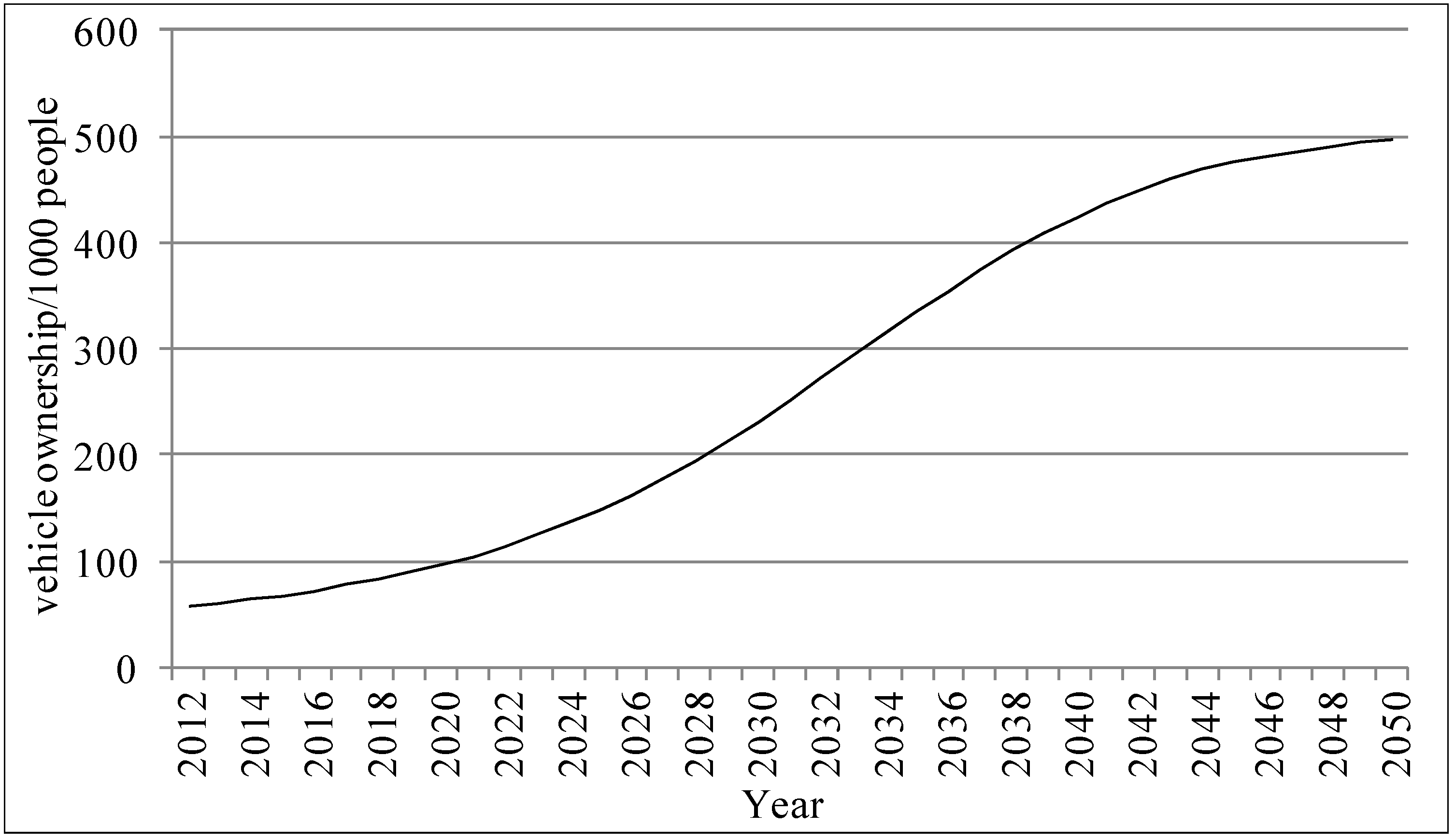
β estimated by the OECD pattern and the annual per capita GDP in China for 2012−2050. Therefore, according to Equation (1), we estimate the vehicle ownership per 1000 people in China from 2013 to 2050 (
Figure 9).
Figure 9.
Annual vehicle ownership per 1000 people in China (2012−2050).
Figure 9.
Annual vehicle ownership per 1000 people in China (2012−2050).
Note: the saturation level of vehicle ownership per 1000 people is 500.
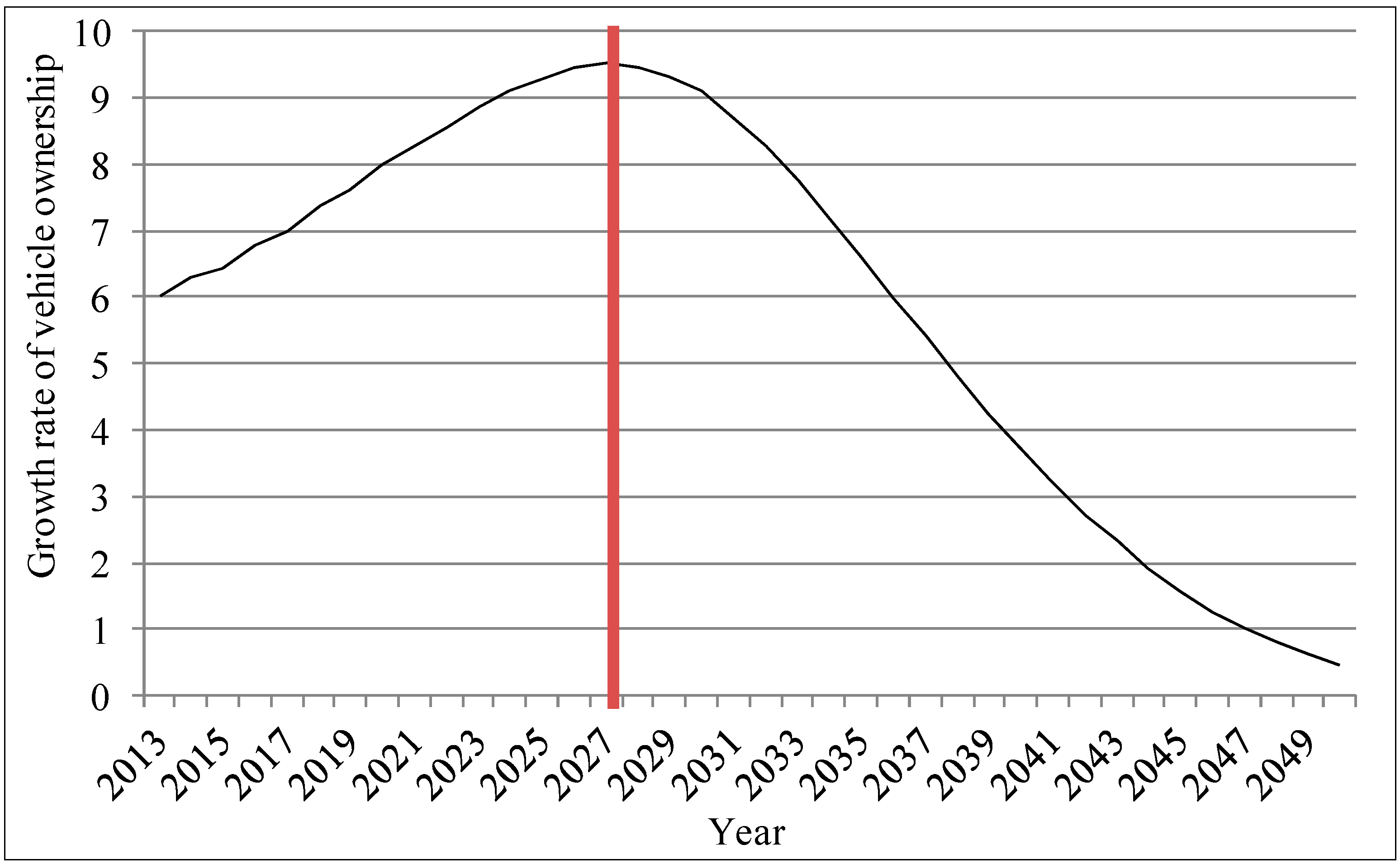
The results show that the growth pattern of vehicle ownership in China depicts an S-shape curve with rapid growth from 2012 to 2027 that then gradually reduces annually, reaching the inflection point of the increasing curve around the year 2030.
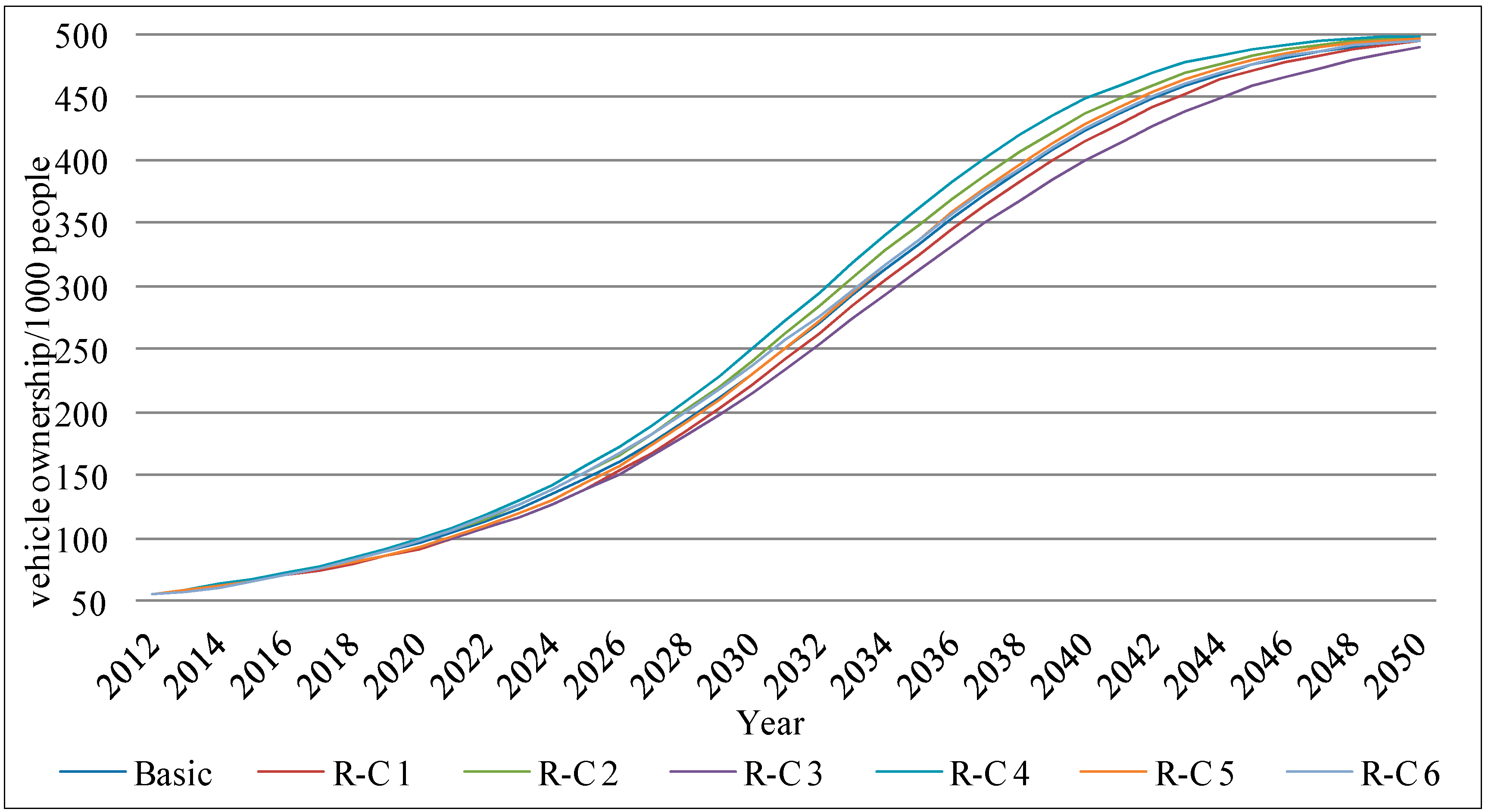
Figure 10 shows the growth of annual vehicle ownership per 1000 people in China.
Figure 10.
Growth of annual vehicle ownership per 1000 people in China (2013–2050).
Figure 10.
Growth of annual vehicle ownership per 1000 people in China (2013–2050).
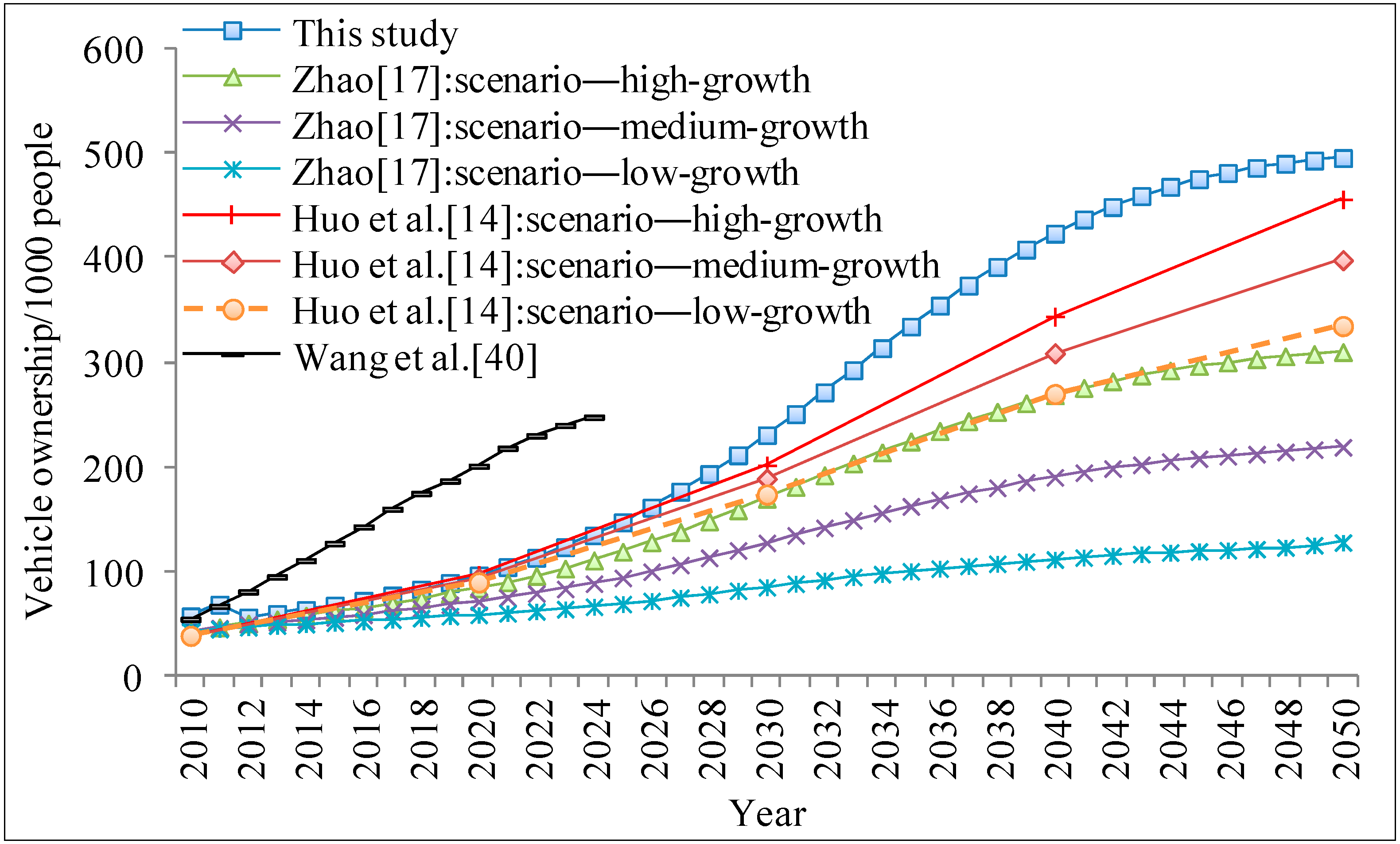
Figure 11 compares the projections on Chinese vehicle ownership per 1000 people made in various studies.
Figure 11.
Comparison of vehicle ownership projections per 1000 people made in various studies.
Figure 11.
Comparison of vehicle ownership projections per 1000 people made in various studies.
As was the case for the vehicle ownership projections shown in
Figure 11, most of the earlier study projections of vehicle ownership per 1000 people are lower than those of this study. The three scenarios applied in Zhao [
17] generated the lowest vehicle ownership levels because the ultimate saturation level of vehicle ownership of China was set at 315 per 1000 people; this may have caused the absolute value of vehicle ownership projection by the Gompertz function in Equation (1). The assumptions of Huo
et al. [
14] on the Chinese annual average GDP growth were overly pessimistic, resulting in lower vehicle ownership projections. However, Wang
et al. [
40] generated a much higher vehicle ownership result than our results from 2010 to 2024. They assumed and mapped a higher GDP growth onto China based on historical growth patterns of a set of countries with comparable growth dynamics; however, they ignored the particularities of China (e.g., the low levels of Chinese per capita GDP and vehicle ownership per 1000 people) and that vehicle stock conforms to the general Gompertz S-shape curve.


 is an AR (1) process.