Article

Minimizing the Carbon Footprint for the Time-Dependent Heterogeneous-Fleet Vehicle Routing Problem with Alternative Paths

1
Department of Tourism Information, Aletheia University, New Taipei City 251, Taiwan
2
Department of Industrial Engineering and Management, National Chiao Tung University, Hsinchu 300, Taiwan
3
Institute of Service Management, National Penghu University of Science and Technology, Penghu 880, Taiwan
4
School of Business, Soochow University, Suzhou 215006, China
*
Author to whom correspondence should be addressed.
Sustainability 2014, 6(7), 4658-4684; https://doi.org/10.3390/su6074658
Submission received: 25 June 2014 / Revised: 13 July 2014 / Accepted: 17 July 2014 / Published: 23 July 2014
(This article belongs to the Special Issue Special issue of Sustainable Asia Conference 2014)

Abstract

:
To respond to the reduction of greenhouse gas emissions and global warming, this paper investigates the minimal-carbon-footprint time-dependent heterogeneous-fleet vehicle routing problem with alternative paths (MTHVRPP). This finds a route with the smallest carbon footprint, instead of the shortest route distance, which is the conventional approach, to serve a number of customers with a heterogeneous fleet of vehicles in cases where there may not be only one path between each pair of customers, and the vehicle speed differs at different times of the day. Inheriting from the NP-hardness of the vehicle routing problem, the MTHVRPP is also NP-hard. This paper further proposes a genetic algorithm (GA) to solve this problem. The solution represented by our GA determines the customer serving ordering of each vehicle type. Then, the capacity check is used to classify multiple routes of each vehicle type, and the path selection determines the detailed paths of each route. Additionally, this paper improves the energy consumption model used for calculating the carbon footprint amount more precisely. Compared with the results without alternative paths, our experimental results show that the alternative path in this experiment has a significant impact on the experimental results in terms of carbon footprint.

1. Introduction

Recently, the global warming has become more and more serious, and each country has paid more and more attention to the related issues of greenhouse gas effects. It cannot be denied that the greenhouse gases due to traffic transportation are harmful to the natural environment. If reckless greenhouse gas emissions continue, irreversible effects in the environment (e.g., global warming, desertification, and a rise in sea level) could result. Reducing the carbon footprint is a direct and effective method for reducing greenhouse gas emissions [1]. According to [2], carbon footprint can be defined as the CO2 emission quantity produced (directly or indirectly) throughout the entire life cycle of a service or a product. Compared with the greenhouse gas emission term commonly used by the public, carbon footprint differs in that it includes all the CO2 emission produced from the extraction and production of the product’s raw materials, production and assembly of the product, and product use, disposal and recycling. Thus, a carbon footprint covers the entire life cycle of a product. Contemporary life is full of environmental pollution, and carbon footprint reduction is necessary to improve the environment for future generations.
According to the investigation by the Intergovernmental Panel on Climate Change (IPCC), transportation accounts for approximately 13% of total greenhouse gas emissions [1]. This means that millions of tons of CO2 are being emitted into the environment, and the numbers are continuing to grow. Therefore, the design of logistics route planning to reduce vehicle exhaust is an effective method for reducing the carbon footprint. The focus of logistics operating system is how effectively to use vehicles. Reducing the number of vehicles through effective vehicle route planning to transport raw materials, semi-finished products, or finished products to their destinations can reduce vehicle exhaust and vehicle transportation costs. Thus, effective vehicle route planning is an important topic in delivery problems. Conventionally, logistics delivery centers determine vehicle routing manually. However, simple manual vehicle route planning methods cannot determine ideal route planning in a short time as a large number of customers and different vehicle fleets are involved. Effective vehicle route planning prior to vehicle assignment can result in the maximal resource utilization effectiveness and drastically reduce vehicle transportation costs. This naturally reduces vehicle exhaust and lowers carbon footprints.
The vehicle routing problem (VRP) is a research topic related to carbon footprint reduction [3]. VRP usually only considers a single depot, vehicle types, and a fixed number of customers. Each customer location has a variety of cargo quantity requirements, and the delivery center is responsible for assigning vehicle fleets with routes to satisfactorily deliver raw materials, finished products, and semi-finished products required by customers. Hence, route planning should achieve many objectives, e.g., the shortest route, the minimal cost, and the minimal required time under certain constraints. However, most practical situations are not as simple as previously described. The situations that affect computational complexity include different vehicle types and capabilities, and different road situations based on time and alternative path selection. How to formulate an effective route in these complex situations has been receiving a lot of attention. Compared with the conventional objectives that involve minimization of time or distance, the VRP with the objective of reducing the carbon footprint is a relatively novel subject. In previous related works on carbon-footprint VRP, Bektaş and Laporte [4] indicated that the factors related to vehicle fuel consumption and CO2 emission, speed, load, distance, and time. Xiao et al. [5] developed an optimization model that adds a new factor, fuel consumption rate (FCR), and uses the simulated annealing method to resolve the model. Their results showed that the fuel consumption for 27 VRPs is reduced by an average of 5%. Although the previous works have addressed the basic VRP, real life VRPs often contain additional variables (e.g., road situations and vehicle types). Since it is unclear whether the basic VRP can be applied to the reality of multiple vehicle types and alternative path selection problems, and the factors in calculating carbon foot prints depend upon different vehicles, vehicle travel speeds, and road situations, most previous works on VRP often only considered a single characteristic, such as vehicle types [6], time-dependent [7], and multiple alternative path selection [8]. However, practical problems often include multiple variables, and applying the VRP that only consider one variable to practical problems may pose difficulties.
To move VRP closer to practical applications, this paper proposes the minimal-carbon-footprint time-dependent heterogeneous-fleet vehicle routing problem with alternative paths (MTHVRPP), which simultaneously considers different vehicle types and alternative path selections, to increase the applicability in practical situations. Since the FCR formula proposed in [5] is not suitable for multiple vehicle types and alternative path selection problems, this paper expands the FCR equation to consider the energy consumption in each time zone of a day, which enables the utilization tour complex MTHVRPP. Furthermore, this paper uses the minimal carbon footprint as the objective to reduce CO2 emission. Compared with the conventional VRPs, the MTHVRPP can be broadly applied to practical situations, which is more in line with real life.
The MTHVRPP differs from conventional VRPs in that the MTHVRPP has different vehicle capacities and travel costs. In conventional VRPs, vehicles are of a fixed type and of a fixed capacity when satisfying the required customer demands; while in the MTHVRPP, the vehicle capacity depends on the vehicle type. Additionally, the conventional VRPs generally have fixed vehicle travel costs; while in the MTHVRPP, the travel costs depend upon the vehicle type, road travel situation, and alternative path selection. Since the VRP is a proven NP-hard problem [9], and the MTHVRPP is an extension of VRP, the MTHVRPP is also an NP-hard problem. As the problem scale expands, the time for finding exact solutions increases with the increases in variables. Compared with the conventional VRPs, the MTHVRPP in this paper additionally considers vehicle types and alternative path selection, which increase the problem-solving complexity. Since typical exact algorithms (e.g., dynamic programming as well as branch and bound) cannot always guarantee finding an optimal solution, effective metaheuristic algorithms are more appropriate for solving large-scale NP-hard problems. In view of the importance of MTHVRPP in actual practice and the problem solving potential of metaheuristic algorithms, this paper uses the genetic algorithm (GA) as the basic framework to develop a problem-solving framework for MTHVRPP, which is expected to achieve an accurate optimal solution efficiently.
The MTHVRPP (which uses the minimal carbon footprint as the objective) concerned in this paper differs from the conventional VRPs (which typically use minimal transportation time and transportation distance as the objective). In addition, this paper proposes a GA to determine appropriate vehicle scheduling to satisfy some practical objectives, such as minimal carbon footprint, minimal total transportation time, and minimal total routing distance. The experimental design is expected to conform to practical problems. Detailed research contributions are given as follows:
  • This paper proposes a GA for minimizing the carbon footprint for the time-dependent heterogeneous-fleet vehicle routing problem with alternative paths (MTHVRPP).
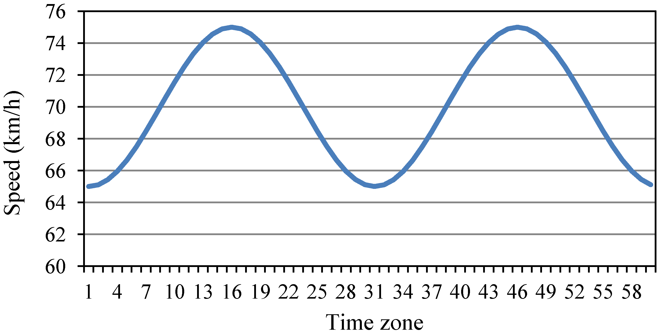
  • In solution representation, time is divided into numerous time steps so that the average vehicle speed on different alternative paths and in different time zones can be expressed.
  • Compared with previous VRPs, the factors that influence carbon footprints such as vehicle type, alternative path selection, vehicle load, and time zone speed are considered in this paper, in order to conform to real life situations.

2. Literature Review
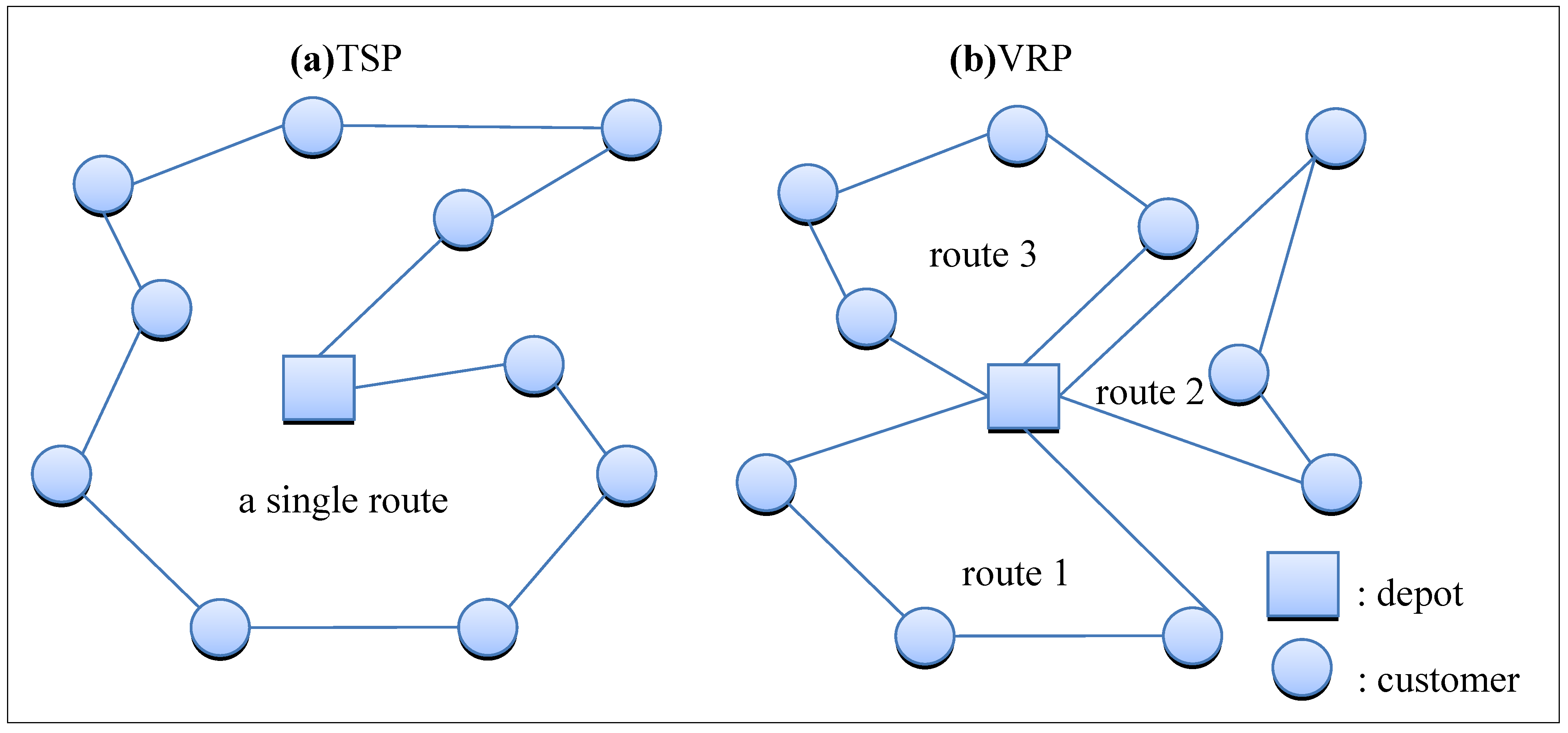
The MTHVRPP in this paper is a type of VRP. This section reviews the previous VRP works related to MTHVRPP, and then the GA.

2.1. VRP

This subsection organizes the previous works on MTHVRPP, such as heterogeneous-fleet VRP (HVRP), time-dependent VRP (TDVRP), and the VRP with alternative paths, and explores their corresponding approaches.

2.2. Description of VRP

Prior to talking about VRP, we must first understand the traveling salesman problem (TSP). The TSP considers a single vehicle that visits multiple customers before returning to the depot, while the total routing time or distance of the vehicle is minimized. Furthermore, when the vehicle capacity limitation is concerned (i.e., the total customer demand requirement of each route of the vehicle cannot exceed the vehicle capacity) this becomes a VRP. The difference between a VRP and a TSP is that a VRP can produce numerous routes to pass through all customer nodes under vehicle capacity limitations. The difference between TSP and VRP is illustrated in Figure 1, in which the TSP is a single-route node-service-combination problem with no vehicle capacity limitation and a VRP is a multiple-route node-service-combination problem with vehicle capacity limitation.
VRP [3] is defined as follows: (1) A vehicle starts from the depot and returns to the depot; (2) the vehicle must satisfy the required demand quantity of each customer; (3) each customer can only be serviced once by the vehicle; (4) the total customer demand quantity serviced by the vehicle cannot exceed the vehicle capacity limitation.
The mathematical model of VRP pursues an optimal vehicle route solution with the minimal total generalized cost that considers practical constraints, e.g., road network characteristics, customer requirements, facility resources, and delivery conditions. The generalized cost refers to the penalty of various negative effects during the vehicle delivery process. A commonly seen negative effect is the transportation cost, which can be divided into fixed cost and variable cost. Fixed costs include vehicle-use costs (e.g., purchase cost and depreciation) and the driver salary, while variable costs are related to delivery route scheduling (e.g., routing distance, time, fuel consumption, and loading/unloading time). Additionally, penalty costs could be generated if delays occur or customer requirements cannot be satisfied.
Figure 1. Illustration of the traveling salesman problem (TSP) and vehicle route problem (VRP) route patterns.
Sustainability 06 04658 g001
Application of VRP in actual practice can derive numerous problem types because of different conditions and changes in limitations, e.g., heterogeneous fleet VRP (HVRP), time-dependent VRP (TDVRP), and VRP with alternative paths. The HVRP differs from conventional VRPs in that it considers more than one vehicle type. Each vehicle type has different cost variables, and the parameters between vehicles are independent [6]. HVRP also does not have limitations on the number of vehicles used [10], and the main objective of HVRP is the maximal utilization of vehicles.
The TDVRP is primarily used in the situation with time window limitations, and its greatest difference from the conventional VRPs is the time change at different customer locations. Specifically, each customer node includes a time window, and the penalty costs could result if a customer node cannot be achieved within the time window [7]. The objective of TDVRP is to arrive at all customer nodes within the time window.
The VRP with alternative paths differs from conventional VRPs in that it has more than one transportation method between customer nodes. Conventional VRPs usually have only one vehicle transportation method. In additional to truck transport, the VRP with alternative paths can transport cargos by trains, airplanes, and other additional transportation methods, and may select more than one path between customer nodes. Regardless of additional transportation method or alternative path selection, the costs for each selection vary [8]. The objective of the VRP with alternative paths is to find one (or multiple) optimal route combinations to obtain an optimal solution. Note that the MTHVRPP proposed in this paper has the problem characteristics of HVRP, TDVRP, and VRP with alternative paths.

2.3. Approaches for VRP

VRP is an NP-hard problem, and numerous previous works existed in the literature. The commonly seen approaches to the VRPs can be classified into mathematical programing and heuristic methods.
In the mathematical programming methods for VRPs, mathematical notations are used to construct high-complexity mathematical models, and then mathematical software is used to obtain the optimal solutions for moderate-size and low-limitation problems within a reasonable time. This method converts the VRP into an easily-solvable mathematical programming model with comparisons for the other optimization works, such as the Lagrangian relaxation method [11], assignment problem [12], set partition problem [13], and set covering problem [14]. However, VRP has numerous related factors in real life that cause difficulties in constructing a mathematical model or is ineffective for large-scale problems. Thus, many previous works have invested in other high-level solution-searching methods or computing technologies to improve this problem.
Since mathematical programming methods may encounter an excessive time consumption bottleneck when solving large-scale VRPs, many previous works have proposed various heuristic algorithms (e.g., generic algorithm, random search strategies, and speculative problem solving methods) to iteratively improve the objective value. This conforms to the practical requirement of efficiently obtaining a solution. The previous works related to heuristics can further be divided into conventional heuristics and metaheuristics.
Conventional heuristics use the greedy method and the local improvement concept to design an easily-implemented problem-solving method, which can generally be discussed in the following two stages: the route construction as well as the route improvement. Route construction is the initial developed heuristic method, which uses its own design rules to complete a possible solution by iteratively considering all the customer nodes to be routed. Clark and Wright [15] used a saving algorithm to calculate the amount of route cost reductions when combining two nodes (while not violating vehicle capacity), and then arranged priority node combinations according to the amount of location savings. Rosenkrantz et al. [16] proposed the insertion algorithm, which starts with a simple route, and then greedily finds the other node with the minimal cost to be inserted into the route until all customer nodes have been serviced. On the other hand, we consider the route improvement stage after the initial route is constructed. At this stage, the nodes and arcs of the initial route are exchanged and rearranged to improve the route solution. Popular route improvement methods include arc exchange and node exchange. The K-Opt arc exchange method proposed by [17] is one of the most commonly-used exchange method, which is based by [18,19,20,21,22].
Metaheuristics use iterative search to randomly jump in feasible solution space, so that the defect of converging on local minimum in conventional metaheuristical gorithms can be eliminated and the solution quality can be improved. Main metaheuristic methods include tabu search (TS), simulated annealing (SA), genetic algorithm (GA), ant colony optimization (ACO), and threshold accepting (TA). TS has a short-term memory effect to avoid repeated searches so that the optimal solution can be approached gradually. SA and TA operate under similar concepts of a certain probability of accepting inferior solutions and escaping local optimal solution constraints to continue searching. GA [23] simulates the genetic evolution process and uses crossover and mutation mechanisms to search for the optimal solution. ACO simulates the habit of ants leaving pheromones, and gives different alternative path selection probabilities for VRP to find superior routes. Many other works have also combined different algorithms to obtain a superior solution. For example, Osman [24] combined TS and SA concepts for the solution search during routing improvement. Van Breedam [25] used three types of routing improvement methods, and then added SA mechanisms for improvements. Tan et al. [26] combined TS, SA, and GA to solve the VRP with time window.

3. Our Genetic Algorithm Approach for MTHVRPP

No previous works have simultaneously considered the VRP with alternative path selection and multiple vehicle type limitations. Thus, alternative paths and multiple vehicle types in this paper are focused to explore VRP road network configuration. By using genetic algorithm (GA) design, we expect to find possible solutions and use these solutions to get close to the optimal solution. The previous works on VRP did not usually consider alternative path selection. Furthermore, the objective of this paper is carbon footprint minimization, and the factors that affect carbon footprints include road conditions, vehicle speed, vehicle load, and the weight of the empty vehicle. Therefore, this paper additionally considers the mechanisms for multiple alternative path selections and multiple vehicle types to conform to the factors that affect carbon footprint. Additionally, as for alternative path selection, different paths have different road conditions, and different vehicles have different capacities and empty vehicle weight. Thus, the focus of this paper is to obtain the optimal solution with the above multiple conditions.

3.1. Problem Description

Derived from the VRP, the MTHVRPP optimization model includes many concepts and limitations similar to typical VRP optimization models. However, since the vehicle and route limitations in MTHVRPP are different than those in VRP, the differences between MTHVRPP and VRP must be explored before constructing the MTHVRPP optimization model. Compared with VRP, the most prominent characteristics of MTHVRPP are as follows:
  • The objective of the MTHVRPP is to minimize the total carbon footprint, not distance or time.
  • The MTHVRPP has more than one vehicle type, and the capacity and basic costs of each vehicle are different.
  • In the MTHVRPP, multiple paths exist between customer nodes; the distance of each path and the speed of different time zones of a day and different vehicles are also different.
  • Because multiple vehicle types exist, the basic costs for each vehicle are different. The carbon emissions also change based on the load and travel speed during the routing trip.
In the conventional VRP model with a single vehicle type, only the road section variables are required to determine whether the vehicle travels on each road section, but the vehicle type traveling on the road is not considered. However, the MTHVRPP requires consideration of multiple vehicle types; therefore, conventional solution representation for VRP cannot easily express the solution characteristics in MTHVRPP.
In addition, note that the MTHVRPP and the conventional heterogeneous fleet vehicle routing problem (HVRP) are also different. Because the conventional solution representation only uses a single path between customers and does not consider alternative path selection problems, additional path selection mechanism in the solution representation compensates for the added alternative paths, which is an important topic in this paper.

3.1.1. Problem Assumptions

To simplify complexity and maintain reasonable cost assumptions, this paper has the problem limitations and makes the following assumptions:
(1)
Route information:
  • There is only a single depot, and its location is fixed.
  • The distance between customers, the customer locations, the customer demand quantity, and the vehicle speed on routes between customer nodes in different time zones are known and fixed.
  • Vehicles leave from the depot and return to the depot after servicing all the customers.
  • The capacities for different vehicles are fixed and known.
  • The total customer demand requirements on each route cannot exceed the vehicle capacity.
  • More than one path between nodes can be selected.
  • Each customer node must be visited, and is only visited once.
  • Different vehicle types can be used for delivery according to the number of the required routes and the routing distance.
(2)
Costs and time:
  • There is a positive proportional relationship between the vehicle routing distance and the vehicle carbon emission.
  • There is a positive proportional relationship between the vehicle load and the vehicle carbon emission.
  • The carbon emission from servicing customers is not considered.
  • The vehicle types and vehicle number limitations are not considered.
  • The routing time of each vehicle is limited.
  • The vehicle fixed costs are not considered.
  • The time window limitations are not considered.

3.1.2. Notations

  • Node information:
    I: I = {V1, V2, V3 ... VS}, where vi is a customer nodes for i ϵ {1, 2, …, S}.
    v0: v0 is the depot node.
    I0: I0 = I ∪ {v0}
  • Vehicle information
    U: The number of vehicle types.
    Au: The surface area of each vehicle type.
    Wu: The empty weight of each vehicle type.
  • Constant
    qi: The cargo demand requirement of node i.
    Zij: The number of selectable paths from node i to node j.
    Qu: The maximum load capacity of vehicle type u.
    Sustainability 06 04658 i021: The speed in time zone m on path z between nodes i and j.
    Dijz: The distance of path z between nodes i and j.
    S: The total number of customer nodes.
    N: The number of vehicle routes.
    Tm: The starting time point for time zone m.
    L : The vehicle routing time limitation.
  • Label
    i, j, k : Node label.
    z : Route label.
    m: Time zone label.
    u: Vehicle type label.
  • Variables:
    s: The number of customers’ nodes that have already been serviced.
    Sustainability 06 04658 i022: The cargo load of vehicle type u on route n after passing node i.
    Sustainability 06 04658 i023 : The time point when the vehicle reaches node i on route n.
    Sustainability 06 04658 i024: The time point when the vehicle leaves node i on route n.
    Sustainability 06 04658 i025: The time consumed by traveling on route n in time zone m on path z between i and j.
    Sustainability 06 04658 i026: The total routing time between nodes i and j on route n.
    Sustainability 06 04658 i027: The routing distance taken on route n in time zone m on path z between nodes i and j.
    Ln: The time traveling on route n.
    Sustainability 06 04658 i028: The total carbon emission of vehicle u between node i and j on route n.
    gn: The total carbon emission on route n.
    TG: The total carbon emission for the entire route.
    TD: The total routing distance.
    TT: The total routing time.
  • Variables:
    Sustainability 06 04658 i029 Sustainability 06 04658 i030
    Sustainability 06 04658 i031 Sustainability 06 04658 i032
Bektaş and Laporte [9] indicated that the amount of carbon footprint is determined by the vehicle energy consumption between customer nodes, as calculated as follows:
Sustainability 06 04658 i001
where Pij is the energy (J) required by the vehicle from customer nodes i to j; w represents the weight of an empty vehicle (kg); fij represents the vehicle load (kg) between customer nodes i and j; dij represents the distance (m) between customer nodes i and j; vij represents the travel speed (m/s) of the vehicle between customer nodes i and j; αij is the specific route-related constant and β is the vehicle-related constant, respectively calculated as follows:
αij = a + gsinθij + gCrcosθij
β = 0.5CdAρ
where a represents the vehicle acceleration (m/s2); g represents the gravitational constant of 9.81 (m/s2); θij represents the road inclination angle between customer nodes i and j; Cr represents the rolling resistance coefficient; Cd represents the road resistance coefficient; A represents the surface area of the vehicle (m2); ρ represent the air viscosity coefficient. However, the aforementioned equation is only appropriate for the ordinary VRP and is not completely suitable for the MTHVRPP proposed in this paper. Thus, we improve the previously described equation and enable the equation to be used in MTHVRPP with different vehicle speeds at different time zones, as shown below:
Sustainability 06 04658 i002
where Sustainability 06 04658 i033 is the energy (J) required by the vehicle type u going from customer node i to node j in time zone m on route n; Wu is the empty weight of vehicle type u (kg); Sustainability 06 04658 i022 is the load (kg) of vehicle type u on route n after passing through node i; Sustainability 06 04658 i021 is the vehicle speed (m/s) in time zone m on path z between nodes i and j; Sustainability 06 04658 i027 is the distance (m) traveled by the vehicle on route n in time zone m on path z between customer nodes i and j. Furthermore, because the surface area of each vehicle type is different, Equation (3) is modified to:
β = 0.5 CdAuρ

3.1.3. Mathematical Model

  • Objective equation:
The objective of our problem is to minimize the amount of the energy used based on the improved equation combined with variables Sustainability 06 04658 i031, which is given as follows:
Sustainability 06 04658 i003
Note that Sustainability 06 04658 i031 is one or zero according to the condition whether vehicle type u has passed through path z between nodes i and j on route n. If the condition is true, then Sustainability 06 04658 i031 = 1; otherwise, Sustainability 06 04658 i031 = 0. Because the result unit obtained by the original objective equation is in J·m2/s2, our requirement is that this unit must be converted to a kilowatt-hour. One liter of gasoline can produce approximately 8.8 kilowatt-hours of energy [9] and approximately 2.32 kg of CO2 [9]. Thus, this objective equation is multiplied with a coefficient of 2.32/8.8/360000.
  • The constraints of vehicle flow rate conservation:
The following constraint ensures that each node is only passed once, where Sustainability 06 04658 i039 represents whether vehicle type u passes node i on route n. If so, then Sustainability 06 04658 i039 = 1; otherwise, Sustainability 06 04658 i039 = 0.
Sustainability 06 04658 i004
The following constraint ensures that the number of vehicles entering and leaving the node is the same.
Sustainability 06 04658 i005
The following constraint ensures that the vehicle does not return.
Sustainability 06 04658 i006
The following constraint ensures that only one path is chosen between nodes.
Sustainability 06 04658 i007
The following constraint ensures that the number of vehicles leaving the depot is N.
Sustainability 06 04658 i008
The following constraint ensures that the number of vehicles returning to the depot is N.
Sustainability 06 04658 i009
  • Vehicle load capacity constraint:
The following constraint ensures that the total cargo requirement on the route does not exceed the maximum vehicle load capacity, where qi represents the demand quantity requirement of each node.
Sustainability 06 04658 i010
  • Vehicle routing time constraint:
The following constraint ensures that the routing time of each vehicle is smaller than the maximum routing time limitation, where Ln represents the routing time of each route n and L is the maximum routing time.
LnL, ∀n = 1, 2, …, N.
  • Definition constraint:
The following constraint ensures that Sustainability 06 04658 i029 only equals 0 or 1.
Sustainability 06 04658 i011
The following constraint ensures that Sustainability 06 04658 i031 only equals 0 or 1. If vehicle u passes through path z between nodes i and j on route n, then Sustainability 06 04658 i040 equals 1; otherwise, equals 0.
Sustainability 06 04658 i012
  • Calculation of parameters:
The following equation calculates the routing time Sustainability 06 04658 i034 in each situation.
Sustainability 06 04658 i013
The following equation calculates the time point Sustainability 06 04658 i035 that the vehicle reaches customer node j on route n, where Sustainability 06 04658 i036 represents the time that the vehicle left node i.
Sustainability 06 04658 i014
The following equation calculates the total routing time Sustainability 06 04658 i037 from node i to j on route n.
Sustainability 06 04658 i015
The following equation calculates the routing distance Sustainability 06 04658 i038 on route n in time zone m on path z between nodes i and j, where Zi,j is the path selected between i and j.
Sustainability 06 04658 i016
The following equation calculates the total time spend on route n.
Sustainability 06 04658 i017
Note that according to Constraint (13), Ln must be smaller than L.

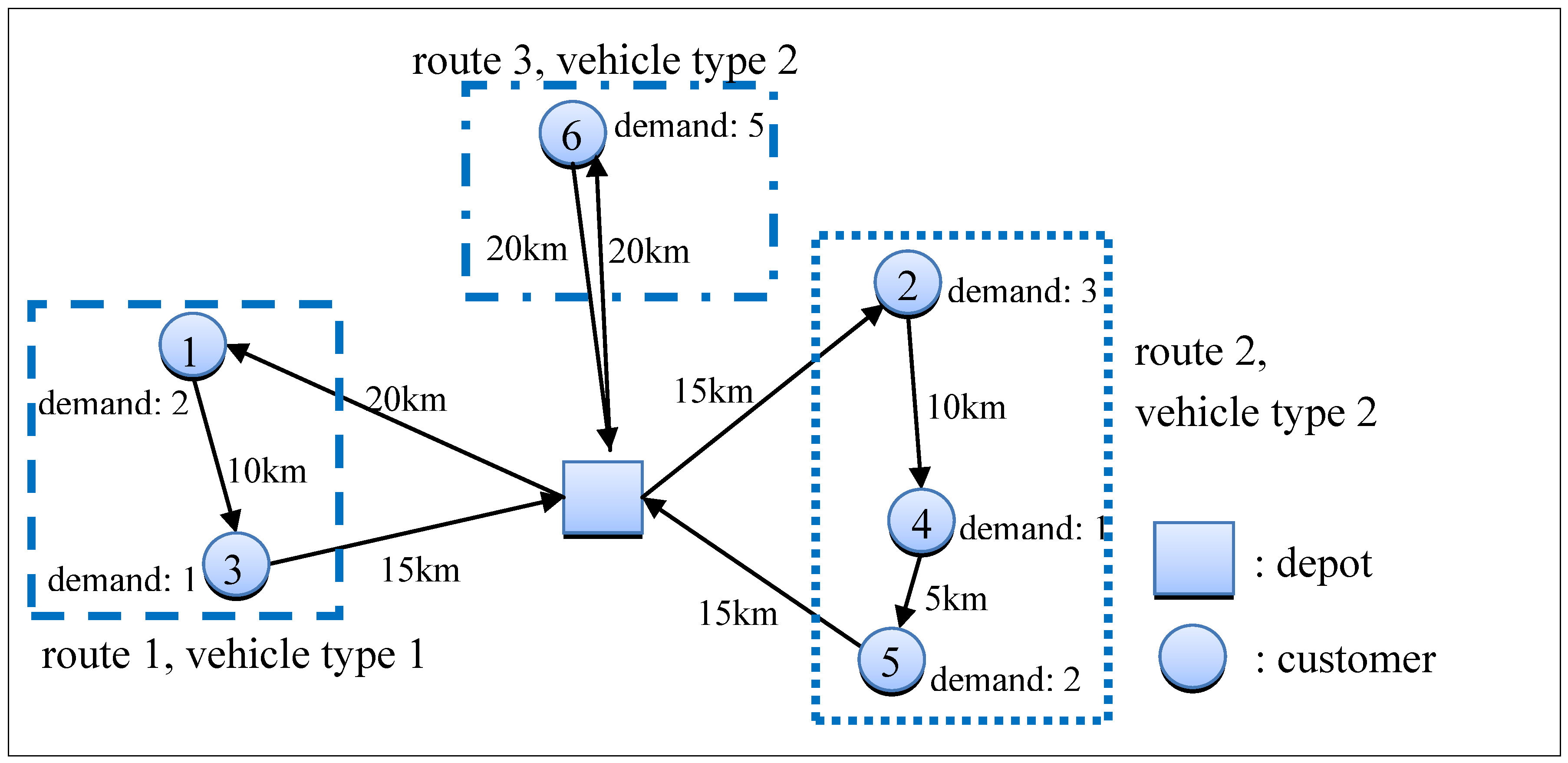
3.1.4. Example Description

We describe a sample problem with five customer nodes and two vehicle types. The locations of the customers and their related distance are shown in Figure 2. We assume that the weights of vehicle types 1 and 2 without cargo loading are 3 tons and 5 tons, respectively. Customer nodes 1 to 6 separately require 2, 3, 1, 1, 2, and 5 tons, and the delivery of those cargos require three routes to be completed. The routing sequence of route1is 0-1-3-0, and requires vehicle type 1. The routing sequence for route2is 0-2-4-5-0, and requires vehicle type 1. Note that the gravitational constant is g = 9.81 (m/s2), the vehicle front surface area A = 5 (m2), the vehicle acceleration speed a = 0 (m/s2), the road inclination angle between customer nodes is θij = 0, the rolling resistance coefficient Cr = 0.01, the road resistance coefficient Cd = 0.7, and the air viscosity coefficient ρ = 1.2041(kg/m3). Detailed calculation for this route configuration is shown in Table 1.
Figure 2. Description of node configuration example.
Sustainability 06 04658 g002

3.2. Genetic Algorithm Design

This subsection states the main components of our GA for MTHVRPP in detail.

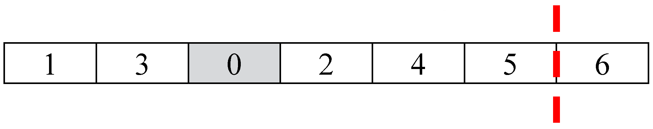
3.2.1. Solution Representation

The solution representation of MTHVRPP is primarily used to determine the route of each vehicle of a different vehicle type (passing each customer node).
Consider the MTHVRPP with U vehicle types and S customer nodes. The length of the chromosome (solution) used in the GA is (U − 1) + S, where U− 1 zeros are used to change vehicle types; the other S numerals are a permutation of numbers 1, 2, …, S, which are used to represent the ordering of the customer nodes serviced. Figure 3 is an example for chromosome expression with 2vehicle types and 6 customer nodes, where 0 separates two sequences of customer permutations that require services, i.e., the first vehicle type delivers to customers 1 and then 3; the second vehicle type delivers to customers 2, 4, 5, and finally 6. Next, our method checks the vehicle capacity. When a vehicle type exceeds its maximum capacity when loading cargos in sequence, a separate route is required. In the example in Figure 3, loads from customers 1 and 2 do not exceed the maximum loading capacity of the first vehicle type. Therefore, the cargo can be transported in one route. However, vehicle type two exceeded its capacity after loading the cargos of customers 2, 4, and 5. Thus, an additional route must be made to load customers 6. In other words, Figure 3 included three routes. Furthermore, our method selects the paths with the least carbon footprint between customers as the final solution.
Figure 3. Description of node configuration example.
Sustainability 06 04658 g003
Table 1. The detailed spreadsheet for the problem in Figure 1.
Time Zone123456
RouteVehicle typePathDistanceWeightSpeedRouting distanceCO2SpeedRouting distanceCO2SpeedRouting distanceCO2SpeedRouting distanceCO2SpeedRouting distanceCO2SpeedRouting distanceCO2Total
n = 1u = 10-1203+3 = 6406.670.41508.330.606050.42 1.45
1-3103+1 = 46050.355050.290.65
3-0153+0 = 3503.330.17406.670.275050.250.7
n = 2u = 20-2155+6 = 10508.330.84506.670.671.52
2-4105+3 = 8401.340.10406.670.51402.000.150.77
4-555+2 = 76050.460.46
5-0155+0 = 5451.330.08457.500.45456.170.370.9
n = 3u = 20-6205+5 = 106010.001.14508.330.84401.670.152.14
6-0205+0 = 54050.27508.330.54606.670.521.35
Total 9.95

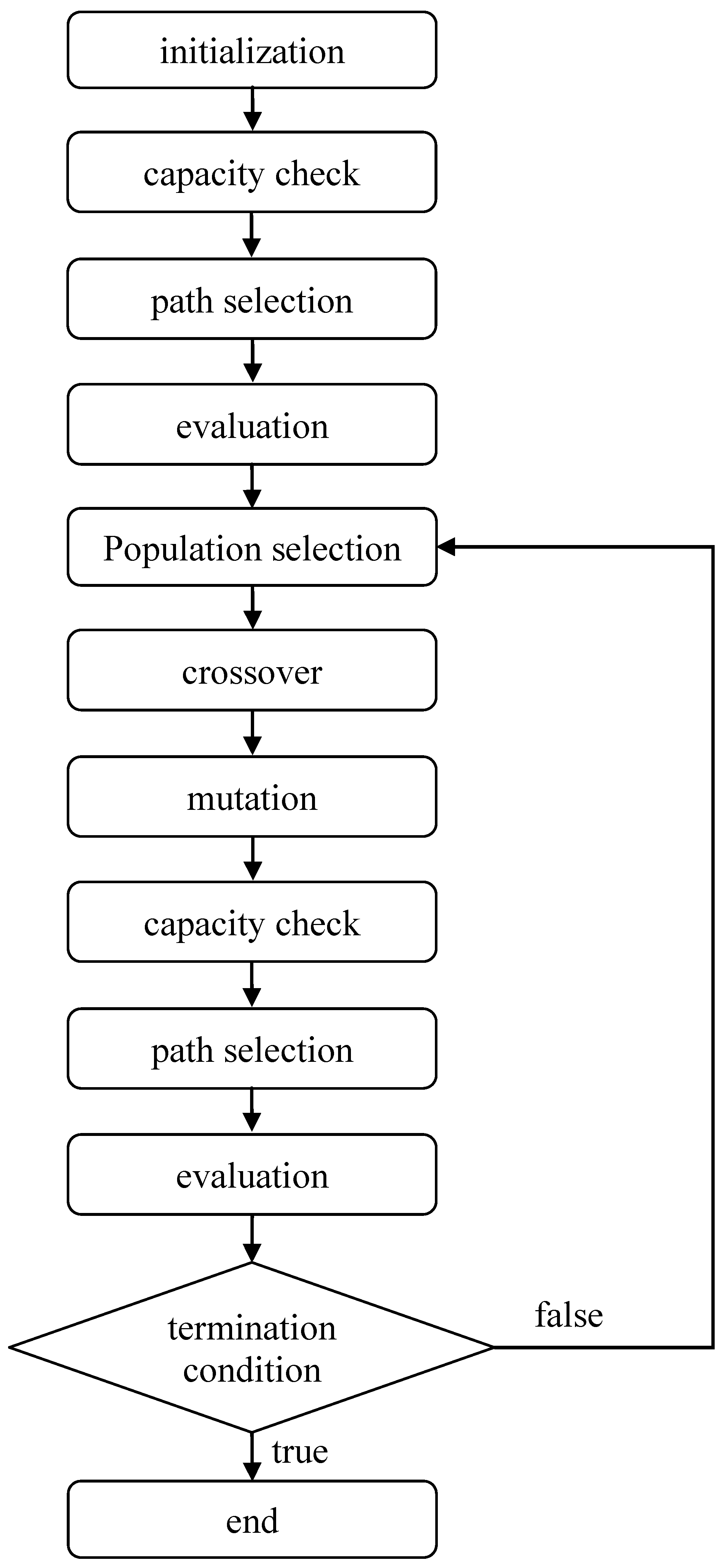
3.2.2. Our Algorithm

Initially, we input all data constants, including customer locations, demand requirements, vehicle type, vehicle capacity, basic consumption, load consumption rate, the distance between nodes, and the vehicle speed on each path within each time zone. When all data has been set, GA is used to solve the problem. The GA process is shown in Figure 4. After the initial group is produced, the GA first starts with a population of chromosomes and evaluates this population. Next, selection, crossover, mutation, capacity check, alternative path selection, and evaluation are repeated until the termination conditions are met.
Figure 4. Our genetic algorithm process.
Sustainability 06 04658 g004
(1)
Initial population
We initialize a number of chromosomes to form a population. When each chromosome is a string of length (U − 1) + S, where U is the number of vehicle types and S is the number of customer nodes. Considering the initialization of each chromosome, each chromosome can be regarded as (U − 1) + S blank spaces. Next, we randomly produce a permutation of 1, 2, …, S, and randomly put the S numbers to these (U − 1) + S spaces. Then, the U − 1 remaining spaces are filled with 0.
(2)
Capacity check
Each chromosome include a permutation of numbers 1, 2, …, S which is separated by U− 1 zeros. That is, a total number of U divisions exist, and the permutation in division i represents the customer service ordering provided by vehicle type i. Next, from left to right, the vehicle type permutation is considered to calculate the loading weight of the concerned vehicle type for the route. If the load of the currently concerned vehicle type exceeds the maximum loading capacity for the vehicle type, then a new route must be considered. Otherwise (i.e., there is no new route generated), we enter the path selection stage and then the fitness evaluation stage. For example, the example in Figure 3 is divided into two divisions: ˂1, 3˃ and ˂2, 4, 5, 6˃. The second division must be divided into two routes because its requirement exceeds the vehicle capacity: ˂2, 4, 5˃ and ˂6˃. In other words, the first vehicle type only has one route: 0-1-3, while the second vehicle type has two routes: 0-2-4-5-0 and 0-6-0.
(3)
Alternative path selection
After completing a capacity check, each route of each vehicle type must be determined. In our problem, furthermore, multiple paths between any two customer nodes can be chosen. Thus, we calculate the carbon footprint of each route between any two customer nodes and then select the path with the lowest footprint as the final route for this chromosome.
(4)
Fitness evaluation
Fitness is primarily used to represent chromosome performance efficacy and as a basis for selecting decisions. The reciprocal of the total carbon emission is used as the fitness in this paper; that is, the smaller the total costs, the higher the fitness value. In case of chromosome i, the aforementioned capacity check and path selection can be used to decide the route and paths of each vehicle type, which can be used to calculate the total carbon emission TG(i). The fitness F(i) is calculated as follows:
Sustainability 06 04658 i018
(5)
Population selection
The primary reason for reproduction is to retain high-performance chromosomes of the parent generation in the new off spring by using the acceleration of the population convergence speed. To match the survival of the fittest and the elimination of the weak when selecting individuals for reproduction, the probability of individuals with large fitness values being selected for reproducing offspring is higher. This paper uses the tournament selection method to make selections. First, two chromosomes are randomly chosen and compared for their fitness. The chromosome with a larger fitness value can proceed with the crossover. This process is repeated until sufficient parent-generation number has been obtained.
(6)
Crossover and mutation
The crossover strategy in this paper is the partially matched crossover (PMX), which is explained as follows. Two parent chromosomes are selected from the parent generation by the above tournament selection. Then, two cutoff points in the chromosome representation are randomly generated, and the partitions between the two cutoff points in the two parent chromosomes are exchanged to reproduce the offspring chromosomes. The genes without conflict from the parent chromosomes are reproduced to the offspring chromosomes. If a conflict exists, then seek other corresponding values for replacement. As for the mutation strategy, we adopt the ordering-oriented mutation, which is explained as follows. Two genes are randomly selected from the chromosomes and their positions are exchanged. A new population of chromosomes is created after crossover and mutation operations are complete.
(7)
Termination condition
Two types of termination conditions exist. The first type is to set the number of maximal generations. If the total generation number satisfies the upper bound, the entire evolutional process is stopped. The second type is the maximum unimproved generation number. If the best fitness value in the latest several generations have not improved (the values converge), the evolution process is stopped.

4. Experimental Design and Results

In this section, the previously mentioned GA approach is tested via a series of experiments. Different costs such as carbon footprint, time, or distance are analyzed and compared with the results of the problems without multiple alternative path selections. The design in this paper refers the model of fuel consumption rate (FCR) developed in [5]. However, because the problem pattern in [5] primarily explored the influence of FCR and the energy conversion effectiveness on energy consumption in different situations (i.e., the experiment and problem pattern is different from that in this paper), it is not compared with our experimental results. Section 4.1 describes the experiment problem instances in this paper. Section 4.2 describes the experimental results of each problem i instance with different objectives and conducts the related parameter analysis on each problem instance. This includes whether routes can be selected, variation of experimental results with different objectives, and combined analysis and comparison of experimental results.
This paper usesC++ program language to implement the proposed algorithm, and all the experiments in this paper are evaluated on PCs with Intel® Core™ (Santa Clara, CA, USA) i7-3610QM CPU@ 2.30GHz 2.30 GHz and memory of 8 GB.

4.1. Description of Experimental Problems and Parameter Setting

Our experimental problems are designed based on those with different numbers of nodes and different vehicle fleet configurations used in [2]. Additional nodes and alternative path selection between nodes are added for different numbers of customer nodes and different vehicle types used for our experiments. An average speed table is established for each route in different time zones.

4.1.1. Parameter Settings

Three experimental problem instances have 20, 50, and 100 customer nodes, respectively, and each customer has a customer label. The x-and y- coordinates of each customer and the customer requirements are known. The number of vehicle types is three or five, and the capacity of each vehicle type is different. Let cS-U denote the name of the experimental problem instance with S customer nodes and U vehicle types. For example, c20-3 represents that the problem instance has 20 customer nodes and 3 vehicle types. Thus, there are six experimental problem instances, i.e., c20-3, c20-5, c50-3, c50-5, c100-3, and c100-5.
The vehicle speed design considers that vehicles have a maximum routing time limitation of 10 h. We define the average vehicle speed to be modified every 10 min. Hence, 60 time zones are planned. Each time zone has a basic speed, which then changes according to the selected vehicle type and the selected route. The basic vehicle speed Vbm for each time zone m is as follows:
Sustainability 06 04658 i019
The above basic speed equation is shown in Figure 5.
Figure 5. Illustration of basic vehicle speeds.
Sustainability 06 04658 g005
Considering that the routing distance affects the road selection, our experiment design categorizes the routes less than 30 km as the regular roads (e.g., highways, county highways and urban roads). Therefore, the vehicle speed is reduced by 20 (km/h), as calculated as follows:
Sustainability 06 04658 i020
Since the alternative path selection is also a consideration factor in this paper, eight possible paths between any two customer nodes are selected in our experiments. Routes1, 2, and 3 allow the basic vehicle speed; routes 4, 5, and 6 allow the basic speed times 0.95; routes 7, 8, and 9 allow the basic speed times 1.05. The distance of each of routes 1, 4, and 7 is the original distance between customer nodes. The distance of each of routes 2, 5, and 8 is 0.95 times the original distance. The distance of each of routes 3, 6, and 9 is 1.05 times the original distance. Vehicle type is also a consideration factor in vehicle speed. Thus, the speed of vehicle types 1 and 2 in our experiment design is 1.025 times faster than vehicle types 3 and 4, and 1.05 times faster than vehicle type 5 (under the same road conditions).
Since the vehicle weight and the maximum load capacity also affect the carbon footprint, our experiment design considers five different vehicle weights and maximum load capacities, as shown in Table 2.
Table 2. Vehicle type classification.
Vehicle typeType 1Type 2Type 3Type 4Type 5
Capacity (ton)11.522.53
Empty vehicle weight (ton)0.7511.522.5
Since the parameters related to the objective function include route-related constant σij, vehicle-related constant β, vehicle acceleration a, road inclination angle θij between customer nodes, rolling resistance coefficient Cr, road resistance coefficient Cd, and air viscosity coefficient ρ, our experiments refer the experimental settings in [4] (as shown in Table 3).
Table 3. Objective-related parameters.
ParameterValue
Vehicle acceleration a0
Road inclination angle θij0.01
Rolling resistance coefficient Cr0.7
Road resistance coefficient Cd0
Air viscosity coefficient ρ1.2041

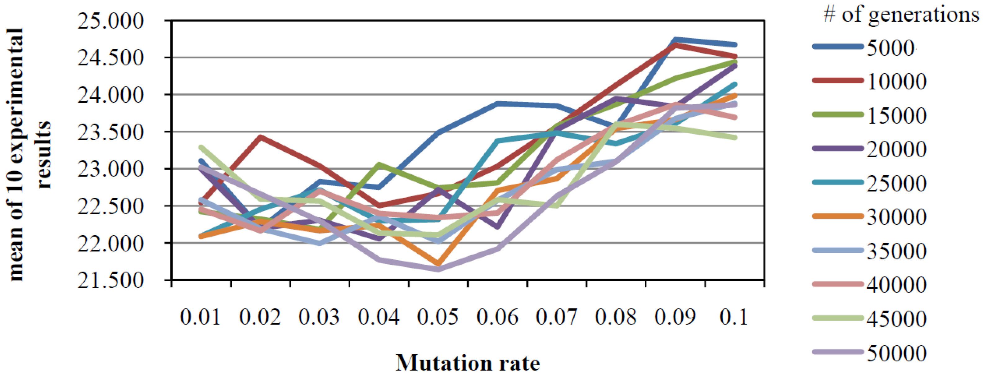
4.1.2. Parameter Setting for our GA

The parameter setting for our GA has a considerable influence on the algorithm. Usually, the more important parameters include the number of generations and the mutation probability. To determine what number of generations and mutation probability can obtain superior solutions; this paper divides these two factors into 10 levels, respectively. That is, the number of generations may be 5000, 10,000, …, and 50,000, and the mutation probabilities may be 0.01, 0.02,…, and 0.1. To find the most appropriate parameter setting for our GA, problem c20-3 is tested, and the objective of minimizing the total carbon footprint is considered. Ten experiments are conducted on each combination of the two factors, and the experimental results are shown in Figure 6, in which the experimental result with the best mean occurs when the number of generations is 50,000 and the mutation probability is 0.05. Thus, this setting is adopted to conduct our subsequent experiments.

4.2. Influence of Different Objectives on Carbon Footprint Emission

This section focuses on changes in number of customers and selectable vehicle types, and determines whether the carbon footprint performance vary when testing different objectives. The Minitab and SPSS system software is used to conduct single-factor ANOVA and independent sample t-test on results of each experimental problem instance with different objectives. In the experiments, we consider the location of each customer, different routing distances, and different speeds in different time zones to conform to practical situations.
Figure 6. Experimental results with different combinations of numbers of generations and mutation rates.
Sustainability 06 04658 g006

4.2.1. Experimental Results

Consider the six aforementioned problem instances (c20-3, c20-5, c50-3, c50-5, c100-3, and c100-5) and design an experiment with three vehicle types transporting to 20, 50, and 100 customer nodes. Ten experiments are conducted with minimum carbon footprint, minimum time, and minimum distance as the objective. Carbon footprint (kg), routing time (minutes), and routing distance (km) results, means, and standard deviations from 10 experiments are obtained. However, because of the page limitation, only the results for problem c100-5are given in Table 4.
Table 4. Experimental results for problemc100-5 with different objectives.
ObjectiveMinimum Carbon FootprintMinimum Routing TimeMinimum Routing Distance
Number of TimesCarbon Footprint (kg)Routing Time (minutes)Routing Distance (km)Carbon Footprint (kg)Routing Time (minutes)Routing Distance (km)Carbon Footprint (kg)Routing Time (minutes)Routing Distance (km)
1201.393522.893466.02221.643118.713286.00222.703045.603162.49
2202.853496.713454.11210.792984.853124.42213.573121.183196.92
3197.753440.533385.34240.773095.693329.09201.783217.583236.93
4198.053415.393355.70224.883019.473173.51213.093215.163290.20
5203.923552.833498.39233.803093.273291.10209.703249.873278.01
6198.693421.673363.89231.073015.333200.99208.123147.693210.50
7203.423494.833484.16219.763123.513256.96218.143156.723228.00
8198.723480.553409.40236.943089.653293.46225.733141.883257.11
9203.533358.023353.18249.573142.633378.40224.073125.423235.01
10187.913194.743130.70231.803136.673349.25217.343092.433185.39
Average199.623437.823390.09230.103081.983268.32215.423151.353228.06
Standard deviation4.79102.87106.1211.2355.6880.407.6561.9440.45

4.2.2. Comparison of Results Obtained with and without Alternative Path Selection Considerations

In this subsection, the SPSS statistical software is employed to compare the experimental results obtained using the models with and without alternative path selection considerations, respectively. The t-tests are conducted to determine whether the carbon footprints yielded from all problem instances are identical when alternative path selection is considered. Table 5 shows the results of the 10 carbon footprint experiments and the means and variances of the results when the minimal carbon footprint is used as the problem objective. The results show that, in all problem instances, the means of the experimental results obtained with alternative path selection considerations are superior to those obtained without such considerations. In addition, according to the ANOVA table of the carbon footprint results for all sample problems, the t-test results for all problems are less than 0.05, indicating a level of significance, i.e., the alternative path selection has a significant influence on the carbon footprint results.
Table 5. Carbon footprint results for all problem instances (unit: kg).
Instancec20-3c50-3c100-3c20-5c50-5c100-5
RouteYesNoYesNoYesNoYesNoYesNoYesNo
122.5322.9382.5189.51195.82202.2921.3023.8083.0088.07201.39212.50
220.5323.2780.1190.28193.65206.0220.0023.5384.5691.24202.85210.07
321.9024.1884.3287.23196.88207.0120.7023.8184.2387.15197.75210.66
421.6324.8582.7785.62197.28207.6420.4822.4079.6489.66198.05212.05
522.6623.6283.0788.28197.74207.5320.8624.5182.2389.99203.92210.04
620.4825.2983.5685.97196.42208.0319.9522.3680.3088.96198.69209.65
722.0124.0482.3290.34196.82207.6821.8122.8783.8591.33203.42203.56
822.8325.7382.8489.35199.21210.2020.8723.2086.1788.93198.72208.24
921.2624.1079.8588.11192.69204.0521.8221.9683.4490.15203.53210.41
1021.5624.2079.2887.71197.23201.4421.7022.7781.1391.70187.91211.31
Average21.7424.2282.0688.24196.37206.1920.9523.1282.8689.72199.62209.85
Standard deviation0.820.871.711.661.922.760.700.792.041.484.792.52

4.2.3. Analysis of the Experimental Results Parameters for All Sample Problems

This subsection presents a single-factor ANOVA regarding the experimental results for problem c100-5. The ANOVA results are used to determine whether various objectives have significant effects on the carbon footprint results. The null hypothesis is that the three objectives have no effects on the carbon footprint results, and the alternative hypothesis is that the three objectives affect the carbon footprint results. The α for the level of significance is set at 0.05 before tests are conducted. When the ANOVA results reach the level of significance, a t-test is conducted between the experimental results obtained using minimal carbon footprint and minimal routing time as the objectives, respectively. The level of significance is set at 0.05. The t-test results are employed to investigate whether the carbon footprints obtained using minimal carbon footprint as the objective are significantly less than those obtained using other objectives.
An ANOVA analysis is conducted using the Minitab and SPSS software to calculate the carbon footprint results for problem c100-5 under various objectives. First, an equality of variance test is conducted to analyze the carbon footprint results under various objectives. The p-value of the test results is 0.65, greater than 0.05. Therefore, the null hypothesis, that is, “H0: The variances of the carbon footprint results yielded under the three objectives are equal”, is not rejected when the level of significance is set at α = 0.05. Thus, considering the homogeneity of the samples, they can be used to conduct a single-factor ANOVA. The results show that the p-valueis0.000, which is smaller than 0.05. Hence, the null hypothesis, that is, “H0: The carbon footprint results yielded under the three objectives are equal”, is rejected when the level of significance is set at α = 0.05. Subsequently, Scheffé’s method is employed to conduct post hoc multiple comparisons. The results show the means of the carbon footprint results obtained under various objectives differ. Finally, a t-test is conducted between the carbon footprint results obtained using minimal carbon footprint as the objective and those obtained using minimal routing time or minimal routing distance as the objectives. The results show that the p-value is 0.000, which is smaller than α = 0.05. Thus, we conclude that when the level of significance is set at α = 0.05, the carbon footprint results obtained using minimal carbon footprint as the objective are significantly smaller than those obtained using minimal routing time or minimal routing distance as the objectives.

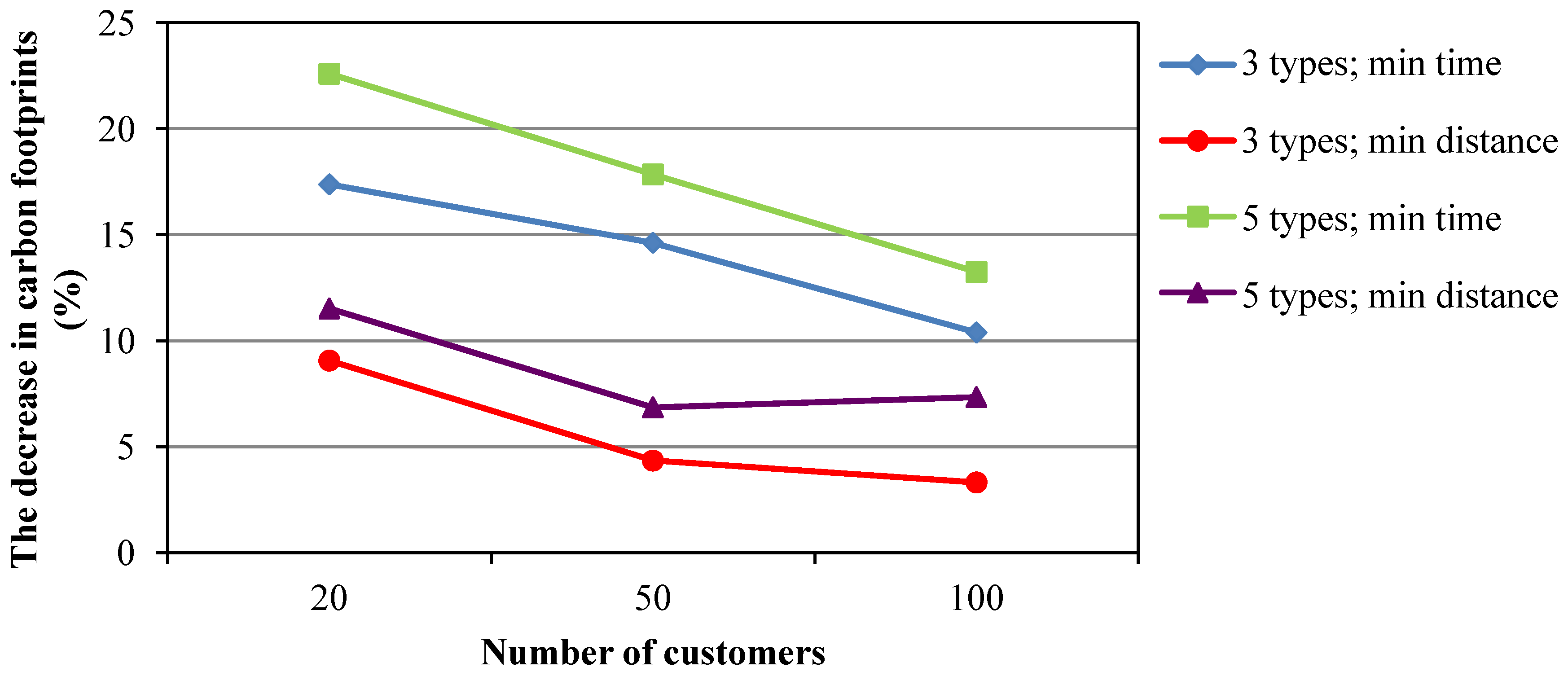
4.2.4. Analysis of the Decreases in the Carbon Footprint Results for All Sample Problems

The means of the carbon footprint results obtained under various objectives are used to explore the decreases in the carbon footprints and to determine whether vehicle types and the number of customers affect the observed decreases. Table 6 shows a comparison of the experimental results obtained for all problem instances using minimal carbon footprint as the objective. Compared with the carbon footprint results obtained using minimal routing time or minimal routing distance as the objective, the results obtained using minimal carbon footprint as the objective are superior in all problem instances although the results have less satisfactory performance in routing time and routing distance.
Figure 7 shows the decrease in carbon footprint as compared with the results obtained using minimal routing time or minimal routing distance as the objectives. The carbon footprint results obtained using minimal carbon footprint as the objective exhibit a satisfactory decrease as compared with the results obtained using minimal routing time as the objective. In contrast, the decrease in the carbon footprint results obtained using minimal carbon footprint as the objective are less satisfactory, as compared to those obtained using minimal routing distance as the objective. The t-test results obtained using Minitab and SPSS statistical software show that when the level of significance is set at α = 0.05, the carbon footprint results obtained using minimal carbon footprint as the objective are superior to those obtained using minimal routing time or minimal routing distance as the objective. Furthermore, the number of customers is a factor that affects the decrease in the carbon footprint results. Figure 7 shows that when the number of customers is 20, the carbon footprint exhibits a more significant decrease compared with those when the number of customers is 50 or 100. Furthermore, the decrease in carbon footprint when the number of customers is 50 is more significant than when the number is 100. In other words, as the number of customers increase, the complexity of the problems rises and the decrease in carbon footprint declines. Although the decrease in carbon footprint obtained using a genetic algorithm declines as the number of customers increase, the experimental results confirm that carbon footprint is reduced effectively. Specifically, the t-test results obtained using Minitab and SPSS statistical software show that the carbon footprint decreases when the significance level of 0.05.
Table 6. Comparison of the results for all problems with objective of minimal carbon footprint.
Problem InstancePerformanceUsing the Objective of Minimal Carbon FootprintComparison to the Results with Objective of Minimal Routing TimeComparison to the Results with Objective of Minimal Routing Distance
MeanMeanDecrease (%)MeanDecrease (%)
c20-3Carbon footprint (kg)21.7426.3117.3823.919.06
Routing time (min)564.09484.4716.43513.84−9.78
Routing distance (km)465.82454.27−2.54445.96−4.45
c50-3Carbon footprint (kg)82.0696.1114.6285.794.34
Routing time (min)1580.701439.02−9.851461.75−8.14
Routing distance (km)1480.491476.98−0.241426.82−3.76
c100-3Carbon footprint (kg)196.37219.1310.39203.093.31
Routing time (min)3441.723129.40−9.983222.66−6.80
Routing distance (km)3401.053288.08−3.443254.69−4.50
c20-5Carbon footprint (kg )20.9527.0722.6023.6811.52
Routing time (min)538.85461.29−16.81482.37−11.71
Routing distance (km)439.12433.76−1.23418.20−5.00
c50-5Carbon footprint (kg )82.86100.8517.8488.956.85
Routing time (min)1575.541387.64−13.541433.68−9.89
Routing distance (km)1477.791441.01−2.551398.84−5.64
c100-5Carbon footprint (kg)199.62230.1013.25215.427.33
Routing time (min)3437.823081.98−11.553151.35−9.09
Routing distance (km)3390.093268.32−3.733228.06−5.02
Figure 7. Comparison of the decreases in carbon footprints obtained using various vehicle types and objectives.
Sustainability 06 04658 g007

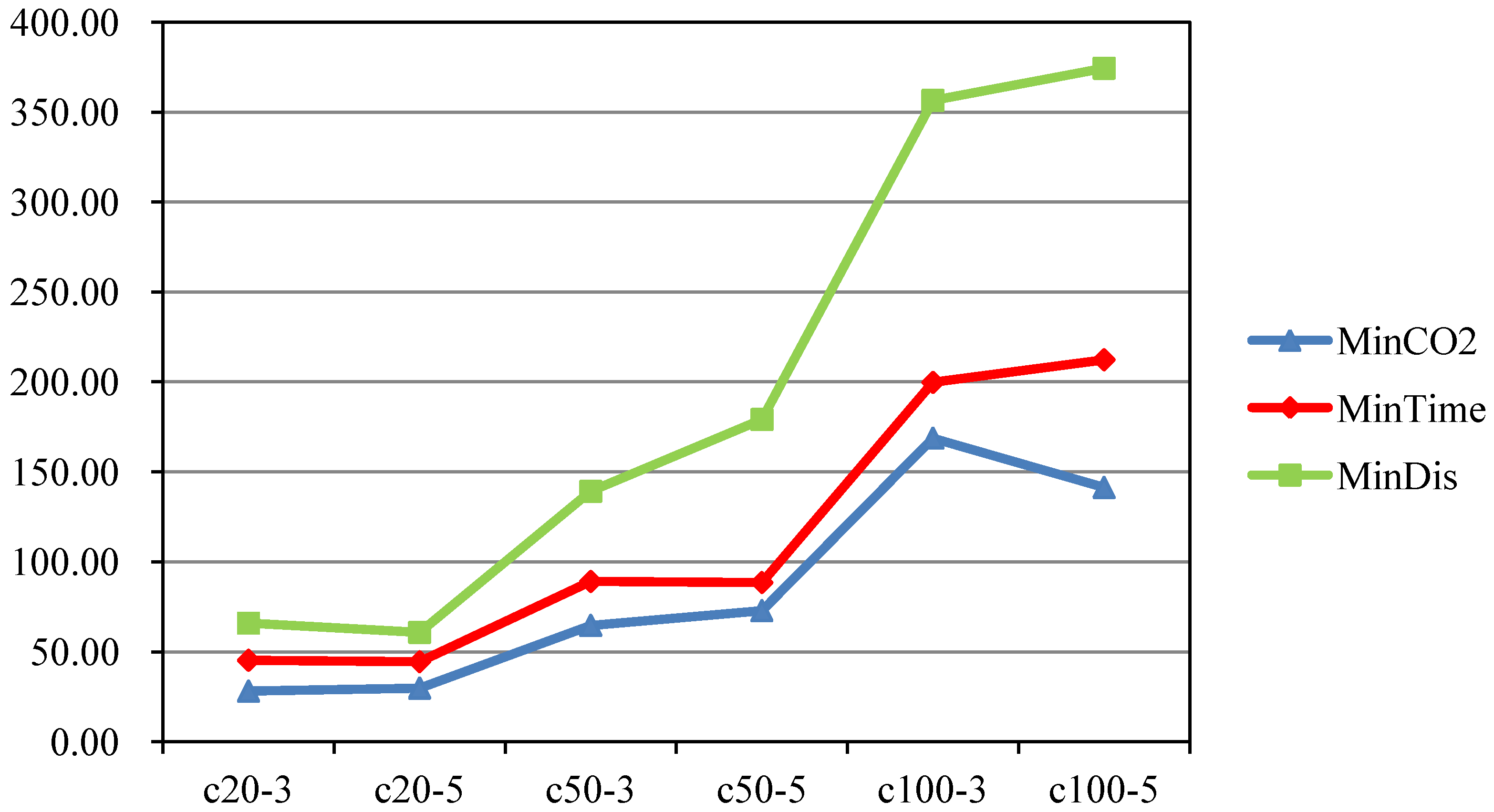
4.2.5. Analysis of the Computational Time Required for Executing our GA

This subsection presents an analysis regarding the computational time required for executing our GA for various objectives in differing problem instances. Figure 8 shows the means of the time required for executing our GA in the 10 experiments for each problem instance. As the number of customers increases, the computational time increases significantly. In addition, a significant difference is observed between the computational time required for solving problems that involve various objectives. The average time required for solving problems that involved minimal carbon footprint as the objective is the shortest, followed in order by the average time required for solving problems that involved minimal routing time and minimal routing distance, respectively, as the objective. From Figure 8, we see that the number of vehicle types has no significant effect on the average computational time.
Figure 8. Comparison of the average time required for solving various problem instances.
Sustainability 06 04658 g008

5. Conclusions and Future Work

VRP is a vital problem in transportation and a crucial link in supply chain management. The problems that involve the basic VRP, and its variants have been investigated and solved in numerous previous works. However, the factors such as vehicle speed, vehicle type selection, vehicle load, and alternative path selection are often overlooked in VRP problems, although these factors often exist in real cases. This paper has developed a genetic algorithm (GA) for solving the MTHVRPP. Thus, the optimal vehicle routing is obtained to achieve the objectives of minimal carbon footprint, routing time, and routing distance. Experimental results confirm that the optimized vehicle routing obtained using the proposed GA yields superior results when the objective is to achieve minimal carbon footprint, although the routing results in relatively long routing time and routing distance. Therefore, determining a balance among various objectives is a critical topic of research.
In addition to the novel solution representation employed for the proposed GA, the concept of vehicle speed in different time zones is proposed, and the approximate optimal solutions are obtained by repeating the crossover and mutation operations in the GA. Based on the various locations of customers, the number of vehicle types, and the vehicle speed in different time zones, the alternative path selection is altered to obtain an approximate optimal solution and to achieve improvements. The results show that the experimental results obtained using minimal carbon footprint as the objective are superior to those obtained using minimal routing time or minimal routing distance as the objective. Furthermore, the decrease in the objective results declines as the number of customers increases. Nevertheless, this means reduced decreases instead of smaller reduced values. In conclusion, the proposed GA can be used to obtain satisfactory feasible solutions.
The main objective of this paper is to design a GA to obtain the vehicle routings that can result in the lowest carbon footprint. However, the objective weights and the relationships among various factors are not investigated. Extensions and improvements are necessary for practical applications. Hence, we offer the following recommendations for future studies. First, the road situations that truly reflect real situations should be explored. For example, real geographical situations can be employed as the samples for environment planning, and the actual change parameters can be integrated to the algorithm. Thus, the feasible solutions obtained can truly reflect the reality. Second, additional constraints can be introduced. For example, the common problems such as the time window problem, penalties, problems that involve multiple depots, and the truck and trailing routing problem can be integrated to enhance the applicability of the algorithm to reality. Third, the multi-objective problem that considers minimization of carbon footprints, routing time and routing distance is also of interest in the future work.

Acknowledgments

The first and second authors (Wan-Yu Liu and Chun-Cheng Lin) were supported in part by National Science Council, Taiwan (NSC102-2633-H156-001 and NSC 101-2628-E-009-025-MY3, respectively). The corresponding author (Qunwei Wang) was supported by the National Natural Science Foundation of China (no.71203151), the Postdoctoral Science Foundation of China (nos.2012M510139, 2013T60561), the Social Science Foundation of Jiangsu Province (no.12GLC008) and the Jiangsu Qing Lan Project.

Author Contributions

Wan-Yu Liu gave the framework of this research. Chun-Cheng Lin constructed the model. Ching-Ren Chiu and You-Song Tsao analyzed the results. Qunwei Wang gave some advices and checked the whole paper.

Conflicts of Interest

The authors declare no conflict of interest.

References

  1. IPCC. Climate Change 2007: Synthesis Report; Intergovernmental Panel on Climate Change: Geneva, Switzerland, 2007; pp. 45–54. [Google Scholar]
  2. Wiedmann, T.; Minx, J. A Definition of ‘Carbon Footprint’. In Ecological Economics Research Trends; Pertsova, C.C., Ed.; Nova Science Publishers: Hauppauge, NY, USA, 2008; Chapter 1; pp. 1–11. [Google Scholar]
  3. Dantzig, G.B.; Ramser, J.H. The truck dispatching problem. Manag. Sci. 1959, 6, 80–91. [Google Scholar] [CrossRef]
  4. Bektaş, T.; Laporte, G. The pollution-routing problem. Transp. Res. Part B Methodol. 2011, 45, 1232–1250. [Google Scholar] [CrossRef]
  5. Xiao, Y.; Zhao, Q.; Kaku, I.; Xu, Y. Development of a fuel consumption optimization model for the capacitated vehicle routing problem. Comput. Oper. Res. 2012, 39, 1419–1431. [Google Scholar] [CrossRef]
  6. Golden, B.L.; Assad, A.; Levy, L; Gheysens, F.G. The fleet size and mix vehicle routing problem. Comput. Oper. Res. 1984, 11, 49–66. [Google Scholar] [CrossRef]
  7. Ichoua, S.; Gendreau, M.; Potvin, J.Y. Vehicle dispatching with time-dependent travel times. Eur. J. Oper. Res. 2003, 144, 379–396. [Google Scholar] [CrossRef]
  8. Garaix, T.; Artigues, C.; Feillet, D.; Josselin, D. Vehicle routing problems with alternative paths: An application to on-demand transportation. Eur. J. Oper. Res. 2010, 204, 62–75. [Google Scholar] [CrossRef] [Green Version]
  9. Coe, E. Average Carbon Dioxide Emissions Resulting from Gasoline and Diesel Fuel, Technical Report; United States Environmental Protection Agency: Washington, DC, USA, 2005. [Google Scholar]
  10. Taillard, E.D. A heuristic column generation method for the heterogeneous fleet. RAIRO Oper. Res. Rech. Opér. 1999, 33, 1–14. [Google Scholar] [CrossRef]
  11. Lenstra, J.K.; Rinnooy Kan, A.H.G. Complexity of vehicle routing and scheduling problems. Networks 1981, 11, 221–227. [Google Scholar] [CrossRef]
  12. Fisher, M.L.; Jaikumar, R. Ageneralized assignment heuristic for vehicle routing. Networks 1981, 11, 109–124. [Google Scholar] [CrossRef]
  13. Bowerman, R.L.; Calamai, P.H.; Hall, G.B. Thespacefilling curve with optimal partitioning heuristic for the vehicle routing problem. Eur. J. Oper. Res. 1994, 76, 128–142. [Google Scholar] [CrossRef]
  14. Cacchiani, V.; Hemmelmayr, V.C.; Tricoire, F. A set-covering based heuristic algorithm for the periodic vehicle routing problem. Discret. Appl. Math. 2014, 163, 53–64. [Google Scholar] [CrossRef] [Green Version]
  15. Clarke, G.; Wright, J. Scheduling of vehicles from a central depot to a number of delivery points. Oper. Res. 1964, 12, 568–581. [Google Scholar] [CrossRef]
  16. Rosenkrantz, D.; Sterns, R.; Lewis, P. An analysis of several heuristics for the traveling salesman problem. SIAM J. Comput. 1977, 6, 563–581. [Google Scholar] [CrossRef]
  17. Lin, S. Computer solutions of the traveling salesman problem. Bell Syst. Tech. J. 1965, 44, 2245–2269. [Google Scholar] [CrossRef]
  18. Baker, B.M.; Sheasby, J. Extensions to the generalized assignment heuristic for vehicle routing. Eur. J. Oper. Res. 1999, 119, 147–157. [Google Scholar] [CrossRef]
  19. Kontoravdis, G.; Bard, J. Improved Heuristics for the Vehicle Routing Problem with Time Windows; Working Paper; Operations Research Group, Department of Mechanical Engineering, The University of Texas: Austin, TX, USA, 1992. [Google Scholar]
  20. Potvin, J.; Rousseau, J. An exchange heuristic for routing problems with time windows. J. Oper. Res. Soc. 1995, 46, 1433–1446. [Google Scholar] [CrossRef]
  21. Russel, R.A. Hybrid heuristics for the vehicle routing problem with time windows. Transp. Sci. 1995, 29, 156–166. [Google Scholar] [CrossRef]
  22. Solomon, M.M. Algorithms for the vehicle routing and scheduling problems with time window constraints. Oper. Res. 1987, 35, 254–265. [Google Scholar] [CrossRef]
  23. Holland, J.H. Adaptation in Natural and Artificial System; The University of Michigan Press: Ann Arbor, MI, 1975. [Google Scholar]
  24. Osman, I.H. Metastrategy simulated annealing and tabu search algorithms for the vehicle routing problem. Ann. Oper. Res. 1993, 41, 421–451. [Google Scholar] [CrossRef]
  25. Van Breedam, A. Comparing descent heuristics and metaheuristics for the vehicle routing problem. Comput. Oper. Res. 1995, 28, 289–315. [Google Scholar] [CrossRef]
  26. Tan, K.C.; Lee, L.H.; Ou, K. Artificial intelligence heuristics in solving vehicle routing problems with time window constraints. Eng. Appl. Artif. Intell. 2001, 14, 825–837. [Google Scholar] [CrossRef]

