1. Introduction
Apart from tradable commodities, such as food, fiber and fuel, agriculture also provides non-commodity outputs. The former production outputs are usually defined as the agricultural economic function. In contrast, the latter are referred to as environmental and social externalities of agriculture, which include agricultural landscapes, farmland biodiversity, water quality, water availability, soil functionality, climate stability (greenhouse gas emissions, carbon storage), food security, food safety, rural viability and farm animal welfare [
1,
2,
3,
4,
5,
6,
7].
Agricultural activities impact upon environmental functions, such as soil function, water purity, air quality, landscapes and biodiversity, resulting in either positive externalities (public goods) or negative externalities (public bad). However, it can be argued that much more negative environmental externalities can be identified than positive externalities, because the current intensive agricultural production systems generate nutrient loading, ammonia emissions, greenhouse gas emissions and biodiversity loss to the environment.
The rural development policy of the EU is a part of the Common Agricultural Policy (CAP), which offers support and encourages the provision of agri-environmental public goods through a range of measures and initiatives [
8]. These initiatives include the implementation and application of agri-environment measures along with area-based payments that incentivize certain land management practices that improve soils, water quality, air quality, habitats and species diversity in addition to the maintenance of the landscape [
9,
10].
The results of a follow-up study on the impacts of agri-environmental measures in Finland [
11] showed that Finnish agri-environmental policies comprised the implementation of the basic, additional and special measures, whereby fertilization levels, fallow areas, grass cultivation and manure handling were targeted to reduce nutrient loads. Other practices, such as crop rotations, organic farming, field margins, filter strips, buffer zones and winter-time vegetation cover were also targeted to promote farmland biodiversity.
According to the current (2007–2013) Agricultural Environmental Schemes (AESs), the 15 Finnish regions investigated in this study received agri-environmental support to a similar extent, because the farms that adopted the basic measure in AESs received fixed and uniform area-based payments. Currently, 90% of Finnish farms participate in these schemes, and 92% of total cultivated areas are enrolled in the AESs. The rate of agri-environmental payment for basic measures is 93 €/ha for crop farmers and 117 €/ha for livestock farmers [
12]. The additional measures yield some additional payment, whereas special support is a cost compensation given to the individual farm based on a cost estimation calculated over several years.
Although many researchers in Finland have examined the Finnish agri-environment situation in terms of a single item, such as water quality, agricultural nutrient runoffs, ammonia emissions, greenhouse gas emissions, rural landscape and farmland biodiversity [
13,
14,
15,
16,
17,
18,
19,
20,
21,
22,
23,
24,
25,
26,
27,
28,
29,
30], there has been relatively few studies in terms of the assessment of the provision of agricultural environment public goods at the regional level. Lankoski and Ollikainen [
31] defined farmland biodiversity and landscape amenities as agri-environmental public goods (i.e., positive externalities) and nutrient runoff as a negative externality in their model that studied endogenous input use and land allocation. In our present study, agricultural nutrient runoffs, greenhouse gas and ammonia gas emissions were categorized as negative externalities of agri-environment, whereas farmland biodiversity conservation was categorized as a positive externality when evaluating the provision of agri-environmental public goods.
We selected specific critical and representative indicators related to water quality, farmland biodiversity, greenhouse gas emissions, ammonia emissions and soil function to evaluate the public goods provision in our study. The study method we used was a synthetic evaluation that included the theory framework of multi-objective decision-making and fuzzy logic.
Fuzzy set theory is best suited for situations in which the parameters being measured involve the use of uncertain and ambiguous information. Thus, the method can interpret the uncertainties of real situations in which the data belong to by ascribing characteristic values with partial degrees of membership. The continuum of membership values lies between zero (full non-membership) and one (full membership) in a fuzzy membership function. Multi-objective fuzzy synthetic evaluation has been widely used to deal with decision-making problems involving multiple criteria evaluation or the selection of alternatives [
32,
33]. Evaluation methods that use fuzzy logic include many different areas of study. For example, environmental suitability assessment [
34], urban air quality [
35], methane generation rate constants in sanitary landfills [
36], mine water inrush sources [
37] and the environment lodging stress for maize planting based on the daily data for weather and soil [
38] can be evaluated by fuzzy logic.
We are not aware of earlier attempts that have applied the use of the fuzzy logic concept for measuring the provision of agri-environmental public goods. When analyzing several parameters numerically that describe various agri-environmental aspects, their data can be condensed into a single value that describes the overall combined level of provision, i.e., into one relative measurement index.
Our study aims (1) to measure whether the provision levels of agri-environmental public goods vary from region to region and (2) to observe how various agri-environmental indicators of different weightings affect public goods and externalities. We suggest that such data provide possible empirical evidence for the future discussion on whether regionally or locally targeted agri-environmental schemes could be useful as a replacement for the current uniformly applied area-based scheme.
This paper is structured as follows:
Section 2 details the reasons for choosing the seven crucial indicators. It aggregates these indicators into a relative index and introduces the evaluation method used in this study. In
Section 3, the results are presented. These are followed by a discussion and concluding remarks in
Section 4.
2. Materials and Methods
2.1. Seven Crucial Indicators Selected and Aggregated for the Synthetic Evaluation of the Agricultural Environment
The main environmental public goods associated with agriculture include improvements in the following: water quality, climate stability, air quality, farmland biodiversity, soil functionality and agricultural landscape; as indicated in the studies by Cooper
et al. [
1], Baldock
et al. [
9], Keenleyside
et al. [
39] and Hart
et al. [
40]. Water quality is heavily influenced by the runoff of nitrogen and phosphorous. The main sources of nitrogen and phosphorus are inorganic fertilizers, organic manures and slurries, livestock feed and silage effluent [
9]. In recent years, the agricultural nutrient surplus balances in the EU have declined because of the decrease in the use of fertilizers, herbicides and pesticides (European Commission, Eurostat). In Finland, both the nitrogen balance and the phosphorus balance have declined over the whole of the 2000–2009 periods (
Appendix Tables A1 and A2).
Greenhouse gases, including nitrous oxide
, methane and carbon dioxide, are emitted through the use of inorganic fertilizers and manures, the use of powered machinery and directly from livestock rearing. Grönroos
et al. [
27] examined the ammonia (NH
3) emission inventory by calculating NH
3 kg output per head (or animal place or pelt) per year and found that livestock, such as cattle, pigs, sheep, goats and horses, are the main animal sources of NH
3 emissions.
Cooper
et al. [
1] indicated that farming systems that were most associated with the provision of public goods include the extensive livestock and mixed system, traditional permanent crop farming and the organic farming system. Those authors used an expert-led assessment of beneficial farming systems and practices to come to their conclusions. Permanent grassland, permanent crops and organic farming not only played an important part in promoting biodiversity interest and soil function, they also contributed to cultural landscapes.
The EU launched the Indicator Reporting on the Integration of Environmental Concerns into Agriculture Policy Operation project (IRENA) that ran from 2002 to 2005. The operation indicators of IRENA agri-environmental indicators included the following: agricultural areas under the Natura 2000 networking program, areas under organic farming, input uses of fertilizer and pesticides, areas of modified land use, such as fallow areas, permanent grassland areas and permanent crop areas, and the measurement of environmental pressure indicators, such as nutrient loading, ammonia emissions, greenhouse gas emissions and biodiversity loss.
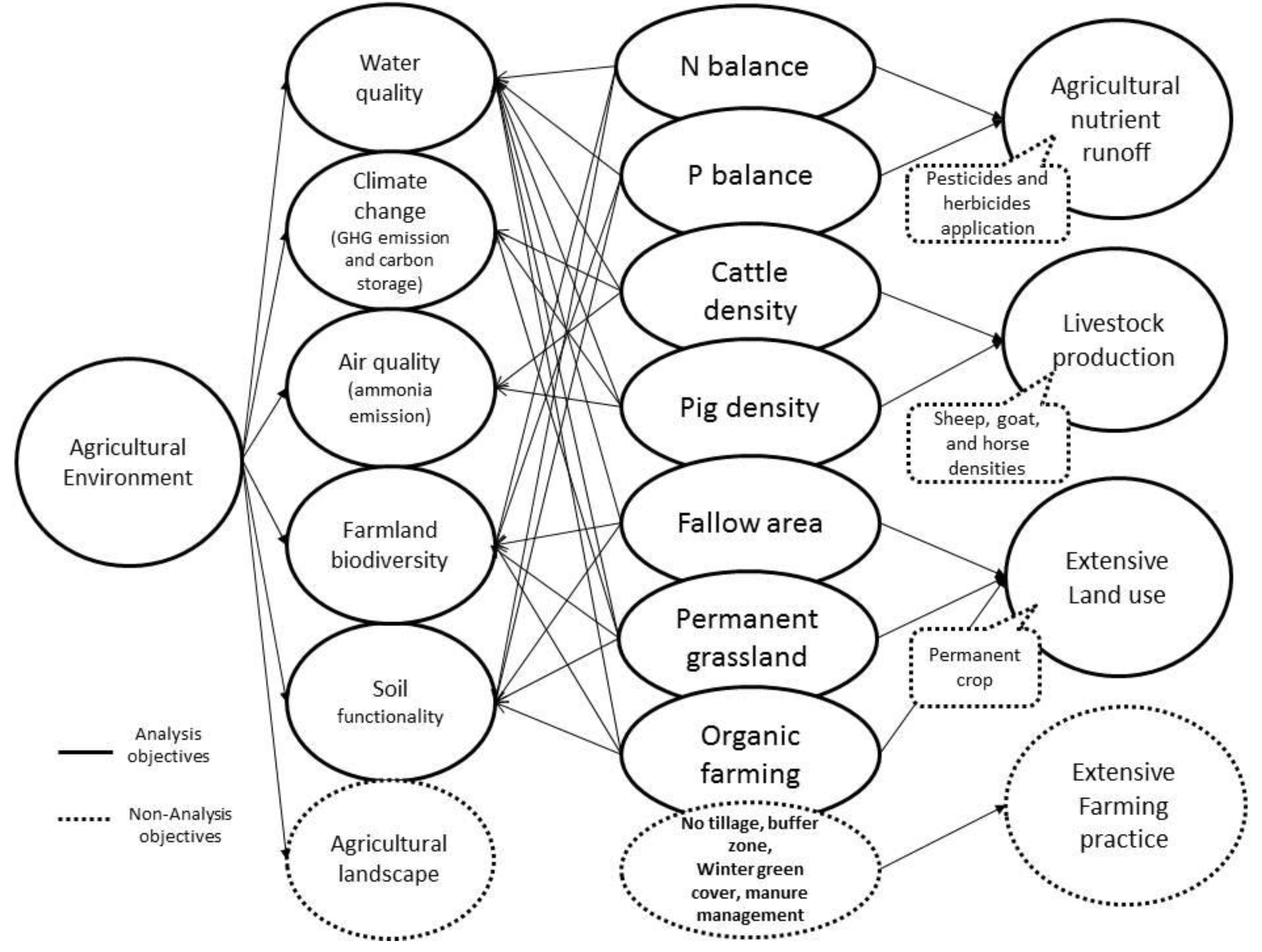
We structured and aggregated agri-environmental indicators into their relationship framework (
Figure 1) based on what was stated above in order to clarify how multiple indicators synthetically evaluate agri-environmental public goods provision.
Figure 1.
Indicators selected in the framework of agricultural environment synthetic evaluation.
Figure 1.
Indicators selected in the framework of agricultural environment synthetic evaluation.
The implementation of some agricultural practices, such as low or zero tillage, the retention of crop residues in fields, buffer strips and zones, winter green cover in fields and appropriate manure management can contribute markedly and beneficially to the agri-environment outcomes. However, complete databases that are related to all those practices are not available at present, which makes it difficult to use them as measuring indicators in the present study. The total amounts of pesticides and herbicides used in Finland were very low, compared to their usage rates in some other European countries, which was mainly due to climatic conditions in Finland. It is also hard to calculate actual usage rates of pesticides and herbicides, because their types are so diverse and the quantities of spray applications for each type vary. The numbers of sheep, goats and horses in Finland were very small compared to those of cattle and pigs (Information Center of the Ministry of Agriculture and Forestry, Helsinki, Finland (TIKE), statistical data during 1990–2010), so these animals could be largely ignored from the ammonia emissions standpoint. Similarly, the permanent crop indicator was not included, because the size of its aggregated area was relatively small (TIKE statistical data during 1990–2010).
Given all the above-mentioned factors, our study used the following seven representative indicators, nitrogen balances, phosphorus balances, permanent grassland proportion, fallow land proportion, cattle density, pig density and organic farming area proportion, to measure the provision levels of agri-environmental public goods. Other possible indicators could have been considered through rough calculations in the future: these include inter alia buffer zone areas, winter green cover areas in fields.
2.2. Statistical Data
The statistical data for nitrogen and phosphorus balances (kg/ha), the densities of cattle and pigs, proportions of permanent grassland and fallow area and organic farming areas in 15 regions of Finland during the 2000–2009 inclusive period were studied. Data were made available from the Information Centre of Ministry of Agriculture and Forestry (TIKE), Agricultural Statistics (Matilda), Statistics Finland, Finnish Food Safety Authority (Evira) and the MYTVAS3 report [
11].
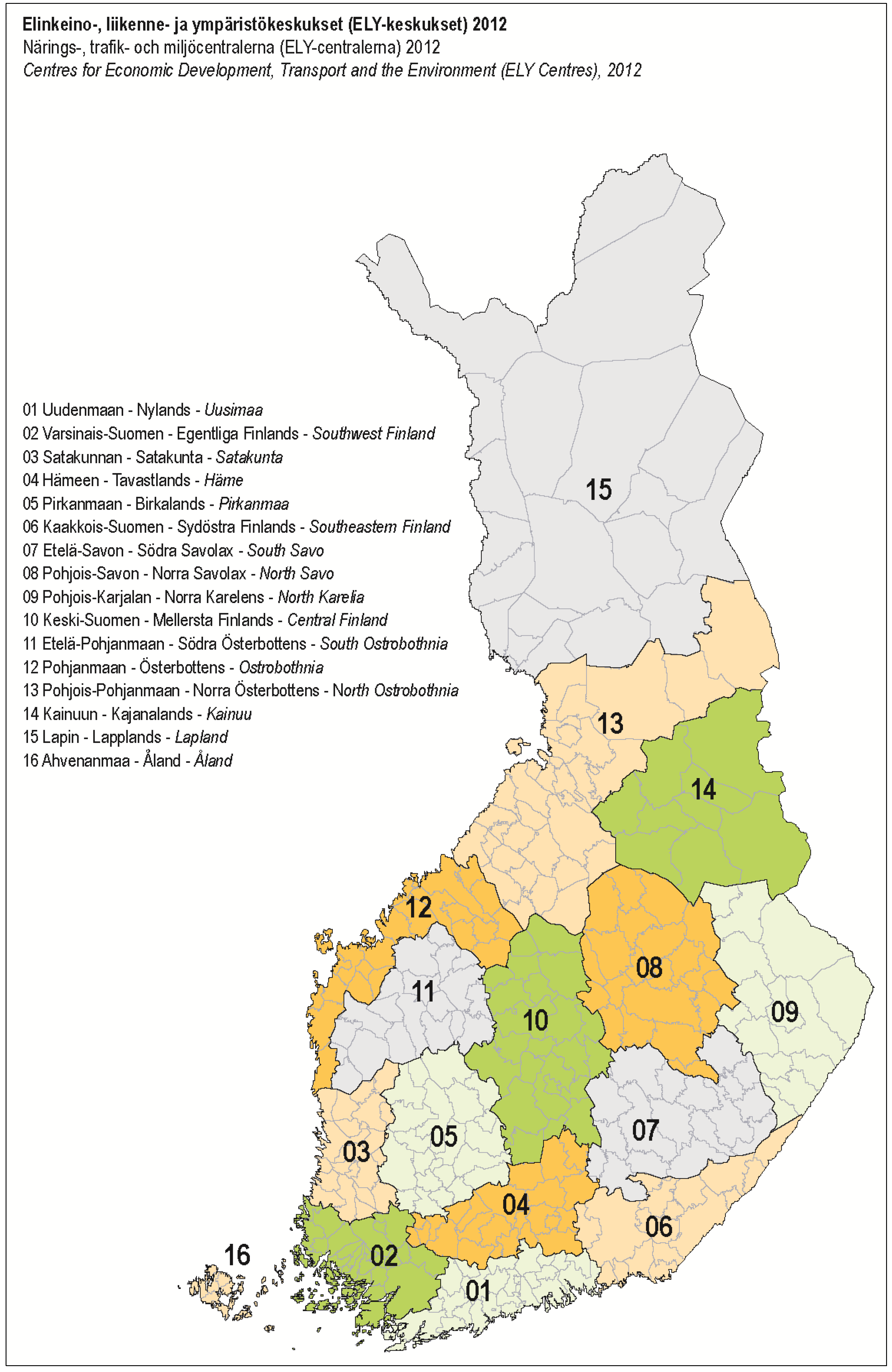
The 15 regions of Finland are named Uusimaa, Southwest Finland, Satakunta, Häme, Pirkanmaa, Southeastern Finland, South-Savo, North-Savo, North Karelia, Central Finland, South Ostrobothnia, Ostrobothnia, North Ostrobothnia, Kainuu and Lapland (
Figure 2). The autonomous Finnish region, Aland, was excluded, because of the lack of data consistency. Regional division is based on the Employment and Economic Development Centers (TE centers) in Finland [
41].
The descriptive results of indicators generally revealed large variations between regions and between years (
Table 1). Only the variation in the proportion of land under permanent grassland was small.
Table 1.
The descriptive statistical data of the selected indicators in 15 regions in Finland (2000–2009).
Table 1.
The descriptive statistical data of the selected indicators in 15 regions in Finland (2000–2009).
| Items | Value | Regions | Year |
|---|
| Nitrogen balance | lowest | 12 kg/ha | Uusimaa | 2009 |
| highest | 83 kg/ha | Ostrobothnia | 2006 |
| Phosphorus balance | lowest | −5.4 kg/ha | Uusimaa | 2009 |
| highest | 14.5 kg/ha | Ostrobothnia | 2004 |
| Ratio of fallow area to utilized agricultural area (UAA) | lowest | 0.004 | Lapland | 2008 |
| highest | 0.145 | Southeastern Finland | 2005 |
| Ratio of permanent grassland to UAA | <0.01 | most regions | 2000–2009 |
| Cattle density (cattle number/UAA) | Low | <0.2 head/ha | Uusimaa, Southwest Finland | 2000–2009 |
| High | >0.8 head/ha | Kainuu, Lapland, North-Savo | 2000–2009 |
| Pig density (pig number/UAA) | lowest | 0.04 head/ha | Lapland | 2009 |
| highest | 2.32 head/ha | Southwest Finland | 2005, 2007 |
| Ratio of organic farming area to UAA | lowest | 0.02 | Häme | 2006, 2007 |
| highest | 0.208 | Kainuu | 2009 |
Figure 2.
The map of the Employment and Economic Development Center showing 15 regions studied (Yearbook of Farm Statistics).
Figure 2.
The map of the Employment and Economic Development Center showing 15 regions studied (Yearbook of Farm Statistics).
2.3. The Method of Synthetic Evaluation
We aggregated the seven agri-environmental indicators outlined above into one synthetic value through the transformations of original indicator values and weightings based on the evaluations of six experts. Let us define the indicator set X: X = (x1, x2, x3, x4, x5, x6, x7), where X was the agri-environmental public goods provision level and xi were the influencing factors.
The indicator values for the factor nitrogen balance, x
1, phosphorus balance, x
2, cattle density, x
5, and pig density, x
6, were transformed by the fuzzy membership function as the following formula:
where xmax was the maximum value for each factor in the 15 regions during 2000–2009 and xmin was the corresponding minimum value. These four factors have negative impacts on agri-environmental public goods provision, thus we denoted the maximum for these factors as a fuzzy membership value of 0, which indicated that it made the least contribution to agri-environmental public goods. We also denoted the minimum as a fuzzy membership value of 1, which indicated that it made the most contribution to the provision of agri-environmental public goods.
The fuzzy membership function values for the factor ratio of fallow area to utilized agricultural area (UAA), x
3, the ratio of permanent grassland area to UAA, x
4, and the ratio of organic farming area to UAA, x
7, could be calculated as the following formula:
Conversely, these three factors have positive impacts on agri-environmental public goods provision. Therefore, we denoted the maximum as a fuzzy membership value of 1 and the minimum as fuzzy membership value of 0.
Combining each single transformed indicator x for each region into the evaluation matrix:
where rij =µ(x), i = 1, 2, …,7 factors and j = 1, 2,…,15 regions.
Additionally, the factor weight set was A = (a
1, a
2, a
3, a
4, a
5, a
6, a
7), where
![Sustainability 06 03171 i004]()
= 1.
Using the weights and indicator values, we calculate the evaluation index as follows:
As a result, we obtained a vector of the regional synthetic index of public goods provision. The index was relative and indicated how close to the maximum value of 1 that a membership value of a particular region was. Thus, it was possible to rank regions using this synthetic index. We noted that the aggregation allowed for the substitution between the indicators. On the other hand, the weights indicated evaluators’ preferences with respect to the recorded indicators.
3. Results
According to the fuzzy membership functions, (1) and (2), Equation (4), and the factor weight set A = (0.2, 0.2, 0.12, 0.12, 0.08, 0.08, 0.2), which was obtained via questionnaire surveys from the six experts in agri-environment or agriculture [
42], we presented the results of the synthetic evaluation indexes (
Table 2).
Table 2.
Regional fuzzy membership values of the evaluation index for 15 Finnish regions (2000–2009).
Table 2.
Regional fuzzy membership values of the evaluation index for 15 Finnish regions (2000–2009).
| | 2000 | 2001 | 2002 | 2003 | 2004 | 2005 | 2006 | 2007 | 2008 | 2009 |
|---|
| Uusimaa | 0.577 | 0.534 | 0.539 | 0.543 | 0.528 | 0.640 | 0.572 | 0.660 | 0.589 | 0.735 |
| Southwest Finland | 0.373 | 0.344 | 0.333 | 0.339 | 0.366 | 0.392 | 0.355 | 0.396 | 0.353 | 0.430 |
| Satakunta | 0.449 | 0.372 | 0.415 | 0.389 | 0.418 | 0.468 | 0.391 | 0.458 | 0.416 | 0.497 |
| Häme | 0.401 | 0.403 | 0.412 | 0.423 | 0.416 | 0.454 | 0.380 | 0.434 | 0.401 | 0.531 |
| Pirkanmaa | 0.475 | 0.475 | 0.500 | 0.480 | 0.468 | 0.541 | 0.433 | 0.509 | 0.460 | 0.591 |
| Southeastern Finland | 0.447 | 0.431 | 0.471 | 0.456 | 0.481 | 0.502 | 0.411 | 0.491 | 0.507 | 0.676 |
| South-Savo | 0.358 | 0.387 | 0.407 | 0.406 | 0.375 | 0.444 | 0.335 | 0.417 | 0.398 | 0.567 |
| North-Savo | 0.290 | 0.299 | 0.337 | 0.330 | 0.329 | 0.426 | 0.326 | 0.364 | 0.345 | 0.461 |
| North-Karelia | 0.361 | 0.400 | 0.448 | 0.474 | 0.459 | 0.499 | 0.487 | 0.508 | 0.479 | 0.610 |
| Central Finland | 0.377 | 0.382 | 0.421 | 0.412 | 0.383 | 0.405 | 0.309 | 0.356 | 0.374 | 0.566 |
| South Ostrobothnia | 0.243 | 0.251 | 0.302 | 0.262 | 0.244 | 0.341 | 0.247 | 0.357 | 0.291 | 0.458 |
| Ostrobothnia | 0.234 | 0.241 | 0.260 | 0.226 | 0.171 | 0.240 | 0.161 | 0.236 | 0.191 | 0.354 |
| North Ostrobothnia | 0.416 | 0.392 | 0.453 | 0.440 | 0.418 | 0.454 | 0.343 | 0.424 | 0.364 | 0.446 |
| Kainuu | 0.372 | 0.379 | 0.484 | 0.437 | 0.447 | 0.549 | 0.494 | 0.539 | 0.523 | 0.659 |
| Lapland | 0.376 | 0.390 | 0.452 | 0.385 | 0.409 | 0.425 | 0.336 | 0.413 | 0.318 | 0.462 |
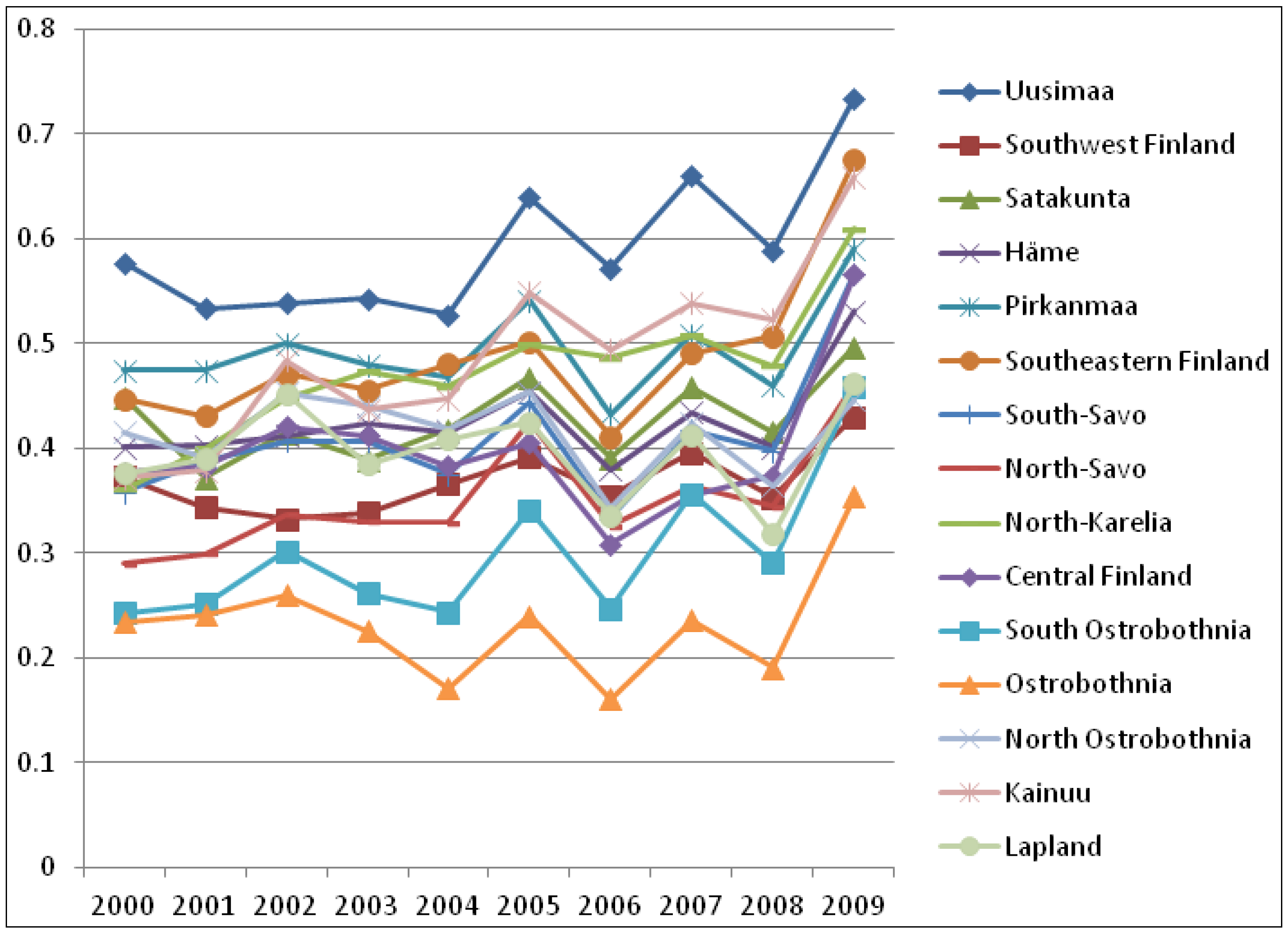
Over that 10-year period, partial membership values of the Uusimaa region remained greater than 0.5. On the other hand, the regions of Ostrobothnia and South Ostrobothnia had relatively low partial membership values from 0.161 to 0.458 (
Table 2). The greater the partial membership value, the better was the provision level. Further, the visually presented results of relative agri-environmental public goods provision levels for all 15 regions studied over the 10-year period are shown in
Figure 3.
The Uusimaa region remained at a relatively high provision level of agri-environmental public goods compared to the other 14 regions in Finland studied for the 2000–2009 period. These relatively high values mainly resulted from low nitrogen and phosphorus balances, a relatively high ratio of fallow areas and low farm animal cattle and pig densities for the Uusimaa region. On the other hand, the regions of Ostrobothnia and South Ostrobothnia had relatively low provision levels of agri-environmental public goods. The main reasons for these inter-regional differences were the relatively high nitrogen and phosphorus balances, high pig densities and low ratios of permanent grassland area in these two regions. The other regions maintained their fuzzy membership values at between 0.3 and 0.5.
Figure 3.
Relative agri-environmental public goods provision levels of all 15 regions in Finland studied during the 2000–2009 inclusive period.
Figure 3.
Relative agri-environmental public goods provision levels of all 15 regions in Finland studied during the 2000–2009 inclusive period.
During the first five years (2000–2004), the trend of agri-environmental provision levels remained relatively stable for all regions. However, a fluctuating, but growing trend emerged for all the 15 regions of Finland studied during the last five years (2005–2009).
Figure 3 shows some differences between regions and years appearing to exist. In order to statistically test whether these differences between regions and between years were significant or not, we carried out a truncated regression with annual and regional dummies (
Table 3).
The index of agri-environmental public good provision was a dependent variable that had a value range of between zero and one, whereas the categorical variables of region and year were independent dummy variables. The truncated regression results (
Table 3) indicated that the indices were significantly different among 15 regions during the 10-year period. Further tests showed that regional dummy values were jointly significantly different from zero. The same was found for the joint significance of the annual dummy value.
We took the Lapland region as a benchmark (
Table 3) and found that the index for the regions of South-Savo, Central Finland and North Ostrobothnia were not statistically different from the reference region. However, with all other regions, the differences were statistically different from the reference region, which was in line with the values on the vertical axis of
Figure 3.
The year 2000 was taken as the base/reference year (
Table 3). We found that the indices for years 2001, 2003, 2004, 2006 and 2008 had no significant differences with that of the reference year, which corresponded to the values on the horizontal axis of
Figure 3. The differences were significant between the years 2000, 2002, 2005, 2007 and 2009.
Further, the test for the trend of the joint environmental performances of Finnish agriculture during 2000–2009 across all regions (the value of the t-test was 3.55, which is statistically significant at the p = 0.001 level) indicated that there has been a marked increase in the provision of public goods, which had developed positively during that decade.
Table 3.
The test (truncated regression) of significant differences for the evaluation index.
Table 3.
The test (truncated regression) of significant differences for the evaluation index.
| Index | Coefficient | Standard error | Z | p > |z| |
|---|
| Uusimaa | 0.1951 | 0.0133 | 14.71 | 0.000 |
| Southwest Finland | −0.0285 | 0.0133 | −2.15 | 0.032 |
| Satakunta | 0.0307 | 0.0133 | 2.31 | 0.021 |
| Häme | 0.0289 | 0.0133 | 2.18 | 0.029 |
| Pirkanmaa | 0.0966 | 0.0133 | 7.28 | 0.000 |
| Southeastern Finland | 0.0907 | 0.0133 | 6.84 | 0.000 |
| South-Savo | 0.0128 | 0.0133 | 0.97 | 0.334 |
| North-Savo | −0.0459 | 0.0133 | −3.46 | 0.001 |
| North-Karelia | 0.0759 | 0.0133 | 5.72 | 0.000 |
| Central Finland | 0.0019 | 0.0133 | 0.14 | 0.886 |
| South Ostrobothnia | −0.097 | 0.0133 | −7.31 | 0.000 |
| Ostrobothnia | −0.1652 | 0.0133 | −12.46 | 0.000 |
| North Ostrobothnia | 0.0184 | 0.0133 | 1.39 | 0.165 |
| Kainuu | 0.0917 | 0.0133 | 6.91 | 0.000 |
| Lapland | omitted | | | |
| 2009 | 0.1529 | 0.0108 | 14.12 | 0.000 |
| 2008 | 0.0173 | 0.0108 | 1.60 | 0.109 |
| 2007 | 0.0542 | 0.0108 | 5.01 | 0.000 |
| 2006 | −0.0113 | 0.0108 | −1.04 | 0.298 |
| 2005 | 0.0687 | 0.0108 | 6.35 | 0.000 |
| 2004 | 0.0109 | 0.0108 | 1.00 | 0.316 |
| 2003 | 0.0169 | 0.0108 | 1.56 | 0.119 |
| 2002 | 0.0323 | 0.0108 | 2.99 | 0.003 |
| 2001 | −0.0046 | 0.0108 | −0.42 | 0.671 |
| 2000 | omitted | | | |
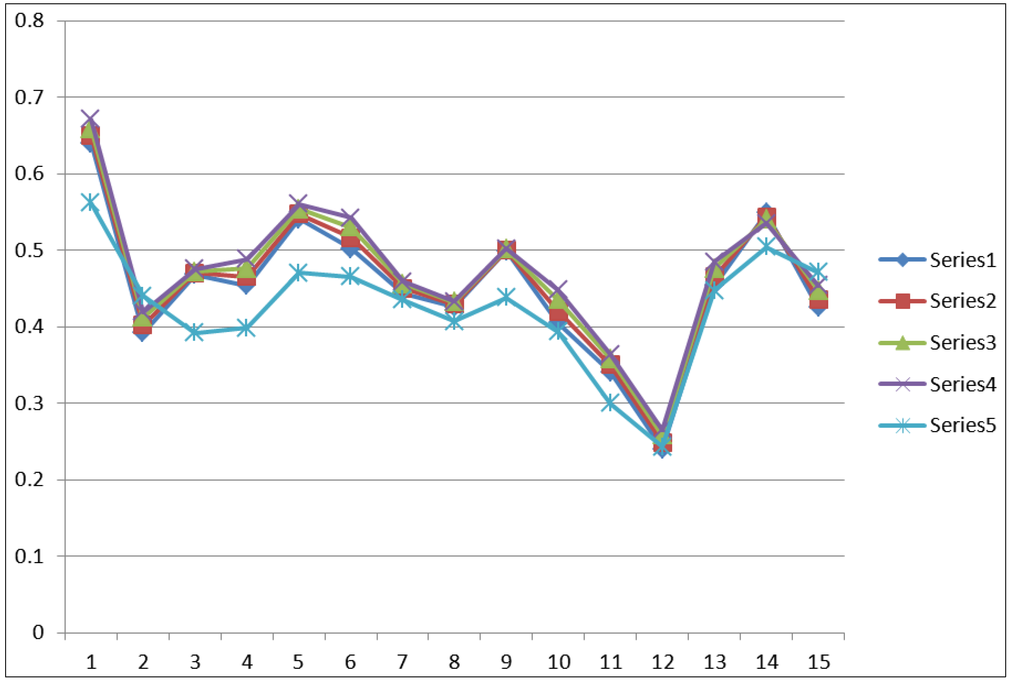
Sensitivity analysis of factor weights:
The factor weights indicated the preferences of the decision-makers. The previous analysis was based on the weightings, which were defined as the mean of values given by a panel of experts. The experts’ preferences were not necessarily equal or even similar. Therefore, we conducted sensitivity analysis with varying factor weightings for our seven indicators. The sensitivity analysis determined that the evaluation results were not sensitive to factor weightings for the following four set types of weighting combinations (
Table 4 and
Figure 4):
-
Decreasing N balance, P balance, organic farming weight by 10% and increasing other factors’ weight correspondingly with the remaining sum of weight of one;
-
Decreasing N balance, P balance, organic farming weight by 20%, increasing other factors’ weight correspondingly with the remaining sum of weight of one;
-
Factor weight is evenly distributed;
-
The weight of N balance: zero.
Table 4.
Sensitivity analysis of factor weights for seven indicators.
Table 4.
Sensitivity analysis of factor weights for seven indicators.
| Sensitivity analysis for factors’ weight | Fuzzy evaluation results in any given year, e.g., (in 2005) | The result order change |
|---|
| Factor weight set derived by experts: (0.2, 0.2, 0.12, 0.12, 0.08, 0.08, 0.2) | (0.640, 0.392, 0.468, 0.454, 0.541, 0.502, 0.444, 0.426, 0.499, 0.405, 0.341, 0.240, 0.454, 0.549, 0.425) | Series 1 in Figure 4 |
| Factor weight change a1 − 10% , a2 − 10%, a3 + 10%, a4 + 10%, a5 + 22.5%, a6 + 22.5%, a7 − 10%: (0.180, 0.180, 0.132, 0.132, 0.098, 0.098, 0.180 ) | (0.650, 0.402, 0.470, 0.465, 0.547, 0.516, 0.450, 0.429, 0.500, 0.420, 0.350, 0.249, 0.465, 0.544, 0.436) | No change (Series 2 in Figure 4) |
| Factor weight change a1 − 20%, a2 − 20%, a3 + 20%, a4 + 20%, a5 + 45%, a6 + 45%, a7 − 20%: (0.160, 0.160, 0.144, 0.144, 0.116, 0.116, 0.16 ) | (0.659, 0.412, 0.472, 0.476, 0.554, 0.530, 0.456, 0.432, 0.501, 0.435, 0.358, 0.258, 0.476, 0.540, 0.447) | No change (Series 3 in Figure 4) |
| Factor weights evenly distributed (each 14.2%) | (0.671, 0.419, 0.475, 0.488, 0.560, 0.542, 0.459, 0.433, 0.502, 0.448, 0.364, 0.265, 0.485, 0.535, 0.454) | No change (Series 4 in Figure 4) |
| Factor weight change with a1 = 0: (0, 0.25, 0.20, 0.30, 0.05, 0.05, 0.15) | (0.562, 0.440, 0.392, 0.398, 0.470, 0.465, 0.435, 0.407, 0.438, 0.393, 0.300, 0.243, 0.447, 0.504, 0.471) | Some differences (Series 5 in Figure 4) |
Figure 4.
Sensitivity analysis of factor weights change.
Figure 4.
Sensitivity analysis of factor weights change.
The results generally showed no significant changes in the ranking of the regions. Thus, the ranking was fairly robust with respect to changes (less than 10%–20% units) in the factor weights. However, when some factor weights differed considerably from the mean values, as in the last case, we could also observe changes in the regional rankings of the provision levels. This indicated that the preferences of experts were also important and should be fully taken into account in the evaluation.
4. Discussion and Conclusions
Our synthetic evaluation of agri-environmental goods provision at the regional level was based on indicators, which represented water quality, soil functional status, greenhouse gas emissions and biodiversity. Our evaluation indicated that the relative provisioning of public goods varies amongst the regions: intensive animal production was one of the main drivers for low provision levels. Intensive animal production typically led to high nutrient balances and a low level of extensive land use. It should be noted that we did not consider the trade-offs between the value of conventional agricultural products and agri-environmental goods provision. Therefore, the provision levels alone cannot be ranked according to their true eco-efficiency values. Moreover, social irreversible costs or benefits from the environmental degradation or its improvement should also be taken into consideration for cost-effective measures, but we did not include this in the model either [
43,
44].
When we compiled our aggregate measure of agri-environmental public goods provision, we used an additive function. In so doing, we assumed that the indicators were fully substitutable for each other. Thus, a decrease in one indicator can be perfectly compensated for by an increase in another indicator under this assumption. In other words, the assumption that the marginal rate of transformation remains constant is crucial to our model. This is a simplistic assumption, but it can be justified when the values of the indicators are close to the normal range, but not when the values are close to the extremes. Otherwise, the shape of the public goods provision is concave to the origin with the slope of the production possibility curve becoming steeper. If the changes in values are substantial, the linearity of the frontier that we assumed may be questioned. We also have to note that the weights that indicate the preferences of the decision-makers affect the rate of transformation.
The highest relative measures of provision we obtained were for Uusimaa, which is the most densely populated region in Finland. High provision levels of public goods are related to the structure of the production systems. When agricultural production is dominated by crops and the common practice of leaving some fields fallow, nutrient balances for crop production also had fewer surpluses than for livestock farming. Support for this can be seen when we compare the data of Uusimaa with those of Southwest Finland and South Ostrobothnia.
The agri-environmental scheme has remained relatively similar over time since Finland joined the EU in 1995. It has been claimed to be relatively ineffective, because it is relatively indiscriminate in its targeting. However, according to our synthetic indicator, the provision of agri-environmental goods has developed positively over the last decade. This positive development is partially linked to adverse price changes in inputs and outputs, which has led to the decreasing use of inputs, such as fertilizers [
45].
Our results obviously reflect the indicators chosen for the analysis. There is a need to mention that we have excluded such environmentally-friendly farming practices as reduced or zero tillage, green field cover in winter, field margins or filter strips, buffer zones, wetland constructions and appropriate manure management. The exclusion of these factors is because of incomplete data at present. We are aware that these farming practices markedly contribute to agri-environmental outcomes. In order to obtain more precise and complete measures of agri-environmental public goods provision in future studies, the area devoted to buffer zones could be calculated in terms of the length of watercourse margins and farmers’ participation rates in the AESs. The area of constructed wetland and winter green cover in the field would be taken into account, as well.
The results of our synthetic evaluation showed that agri-environmental public goods provision levels for 15 regions of Finland during 2000–2009 did fluctuate. Regional differences were statistically significant in many cases. The Finnish agri-environmental support policy has remained roughly the same since it was originally implemented in 1995. Its main goal is to reduce nutrient runoffs from the fields in addition to maintaining agricultural landscapes and biodiversity. However, achievements in reducing nutrient runoff have been very modest according to empirical studies [
46]. Ollikainen
et al. [
47] reported that policy-related transaction costs in the Finnish AESs, especially those incurred by monitoring the basic measures, turned out to be low. This finding implied that an inadequate monitoring effort could not meet the need of the enforcement of the agri-environmental measures. Vehkasalo
et al. [
48] proposed that agri-environmental payments should be differentiated on the basis of the potential environmental benefits provided by different field parcels of land. For example, parcels of land close to watercourses that qualify for fertilization restrictions should also receive higher payments. Support for such a claim can also be found in the study by Beckmann
et al. [
49], who reported a strong demand from experts and stakeholders for the regionalization of the AESs in Finland and other European countries.
The MYTVAS3 report (2007–2013) showed that a relatively high nitrogen balance occurred in the Archipelago Sea and the Bothnian Bay catchments and that a relatively high phosphorous level was found in the Bothnian Bay and Gulf of Bothnia catchments. The flux of phosphorous via the river catchments to the Baltic Sea decreased in all areas except in the sea around the Archipelago over the study period. In contrast, the Gulf of Finland was found to have both low nitrogen and phosphorus levels. Areas of fallow and permanent grass were closely associated with a decrease in nutrient load. However, clustered livestock production units in some regions formed specific nutrient runoff hotspots due to the increased levels of manure produced per hectare from these sites. Our results showed significant differences in public good provision between some regions, but not between all. For this reason, there is likely to be a need to adjust future measures and support levels associated with the agri-environmental program to the needs of each region. These adjustments must be made at the level of different types of farming systems and even for individual farms.
The synthetic evaluation index in our study offers an alternative analytical approach to evaluate the provision of public goods from agriculture. Although it is a relative measure, this index enables the description of the aggregated effects of several externalities generated by agricultural activities in a concise way. It can probably be regarded as one complementary tool for agricultural policy makers to use when they evaluate the provision of agri-environmental public goods and externalities and also when they evaluate the effects of policy changes.


 = 1.
= 1.

