Analysis of Spatial Disparities and Driving Factors of Energy Consumption Change in China Based on Spatial Statistics

Abstract

The changes of spatial pattern in energy consumption have an impact on global climate change. Based on the spatial autocorrelation analysis and the auto-regression model of spatial statistics, this study has explored the spatial disparities and driving forces in energy consumption changes in China. The results show that the global spatial autocorrelation of energy consumption change in China is significant during the period 1990–2010, and the trend of spatial clustering of energy consumption change is weakened. The regions with higher energy consumption change are significantly distributed in the developed coastal areas in China, while those with lower energy consumption change are significantly distributed in the less developed western regions in China. Energy consumption change in China is mainly caused by transportation industry and non-labor intensive industry. Rapid economic development and higher industrialization rate are the main causes for faster changes in energy consumption in China. The results also indicate that spatial autoregressive model can reveal more influencing factors of energy consumption changes in China, in contrast with standard linear model. At last, this study has put forward the corresponding measures or policies for dealing with the growing trend of energy consumption in China.

1. Introduction

The changes in energy consumption have obvious impacted on the pattern of carbon dioxide emission and then on the process of global climatic change [1,2]. Furthermore, China is a country with huge amounts of energy consumption because of its rapid urbanization and industrialization [3,4,5,6,7]. With China’s rapid economic development, energy consumption shows a rapid growth trend [3,8,9,10]. How to maintain higher economic growth and lower energy consumption is the great concern in China. Currently some studies on the energies in China are mostly concerned with the distribution of energy industry in China, sustainable development strategy and construction of energy safety systems and so on [3,11]. The behavior of energy consumption is affected by the economic environment and spatial distance-related migration costs, which has strong geographical features [12]. There is no enough attention to the spatial spillover of energy consumption and its influencing factors. So it is important to explore the characteristics, rules and spatial pattern of energy consumption change in China. However, it is mostly supposed that the relationship between spatial entities is independent when the traditional methods are adopted to measure the spatial disparities of regional changes in energy consumption. In addition, the effect of the spatial correlation had not been focused on enough. Therefore, it is difficult to reflect the global disparities and local spatial heterogeneity in regional changes in energy consumption. Some scholars have begun to find that spatial effect on energy consumption behavior cannot be ignored, and have conducted some empirical tests [9,12,13]. Their studies show the provincial regional economic development and energy efficiency have obvious spatial correlation and cluster in the geographical space, the latter is influenced by its own economic development and the energy efficiency of neighbor region [13]. Meanwhile, other studies also show that there is statistically significant spatial panel autocorrelation for Chinese provincial economic growth and energy consumption [14,15].

Spatial analysis is statistically important because it enhances the inference accuracy, and at the same time it reduces estimated bias with paying enough attention to consider spatial proximity and dependence. Spatial autocorrelation, defined as the situation in which the value of a variable at a location is related to the values of the same variable at the locations nearby, is a statistic method being used to describe spatial interaction of regional social economic phenomena [16,17,18,19,20]. Exploratory spatial data analysis (ESDA), an extension of exploratory data analysis (EDA), is used to detect spatial properties of data and spatial patterns in data, then to formulate hypotheses based on, or which are about, the geography of the data and to assess spatial models [18,21]. Through the description and visualization of spatial information, exploratory spatial data analysis (ESDA) is to explore the spatial agglomeration and anomaly and to reveal the activation mechanism of research object. With it putting forward quantitative measurement of spatial relationship, which is the spatial weight matrix, exploratory spatial data analysis (ESDA) provides a new way to quantity the regional spatial disparities, and it contributes a lot to the highlight of the potentially interesting features in the data and the facilitation of the discovery spatial process [19].

Spatial autocorrelation, the measurement of clustering degree in the spatial domain, serves as the proxy for the correlation of same variables in the different spatial position [22]. Spatial dependence is described by the indicators including Moran’s I, Geary’C, which is classified into global and local indicators [23]. Global indicators are used to verify space model of some social economic phenomena in the whole study area, while local indicators are used to reflect the correlated degree of the certain social economic phenomena or attribute between the sub-region unite and its’ surrounding ones [24]. Because global Moran’s I cannot be used to explore spatial association mode of energy consumption change between neighboring area, and local spatial autocorrelation coefficient acts as the optional measuring index [24]. Exploratory spatial data analysis (ESDA) and spatial autoregressive model are now widely applied to many fields including the economic development disparities, spatial structure of urban development, agricultural development, eco-risk analysis, land use change and energy intensity [17,25,26,27,28,29].

The economic relationship between adjacent regions in China is very obvious, especially frequent mobility of labor, capital and other factors between neighboring provinces [13]. The trades, the spatial associated relationship of industrials, and the spillover of environmental public policy between regions have made the spatial effects of energy consumption obvious from the influence of adjacent regions. In addition, some independent variables including economic growth and population growth also reflects positive spatial correlation. Therefore, spatial auto-regression should be considered in analyzing the influencing factors of energy consumption change in China. The local indicators of spatial association (LISA) clustering plot is used to measure the local spatial heterogeneous and to diagnosis the hot spot and cold spot of spatial clustering about energy consumption change in the local space. This is useful for governments to put forward the targeted policies for energy use in China.

The main purposes of this study are: (1) to explore the spatial correlation and spatial heterogeneity of energy consumption change in China; (2) to find the main influencing factors of energy consumption change in China; (3) and to test the superiority of spatial autoregressive model by comparison with the traditional linear regressive model.

2. Materials and Methods

2.1. Data

Energy consumption data and social-economical data at the province level in this study were derived from the Chinese energy statistics yearbook and the Chinese statistics yearbook from 1991 to 2011, respectively. With the missing data of energy consumption in the Tibet province, Taiwan, Hong Kong and Macao, the final number of spatial analysis unit totals 30 in this study. In this paper 2000 was the year used as the breakpoint, the study period are divided into two periods 1990–2000 and 2000–2010. This is mainly because 2000 is not only the starting point of China’s 10th five-year plan, but also the key year of China's rapid economic development and energy consumption change.

2.2. Methods

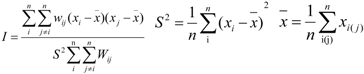
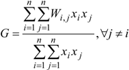
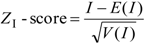
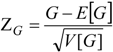
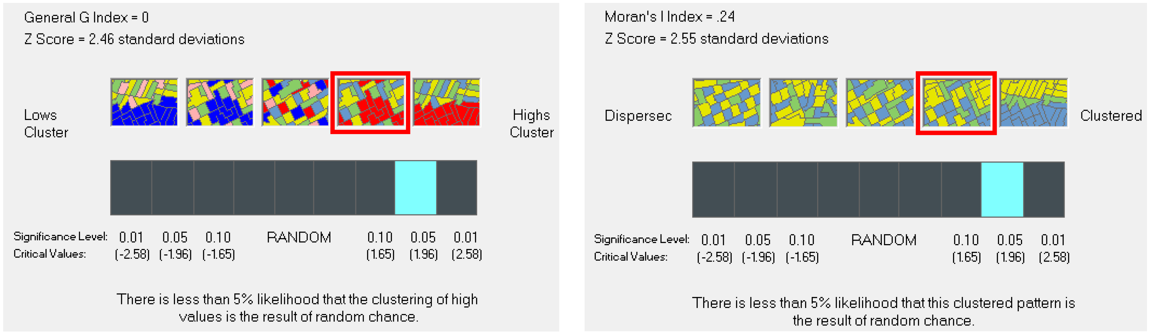
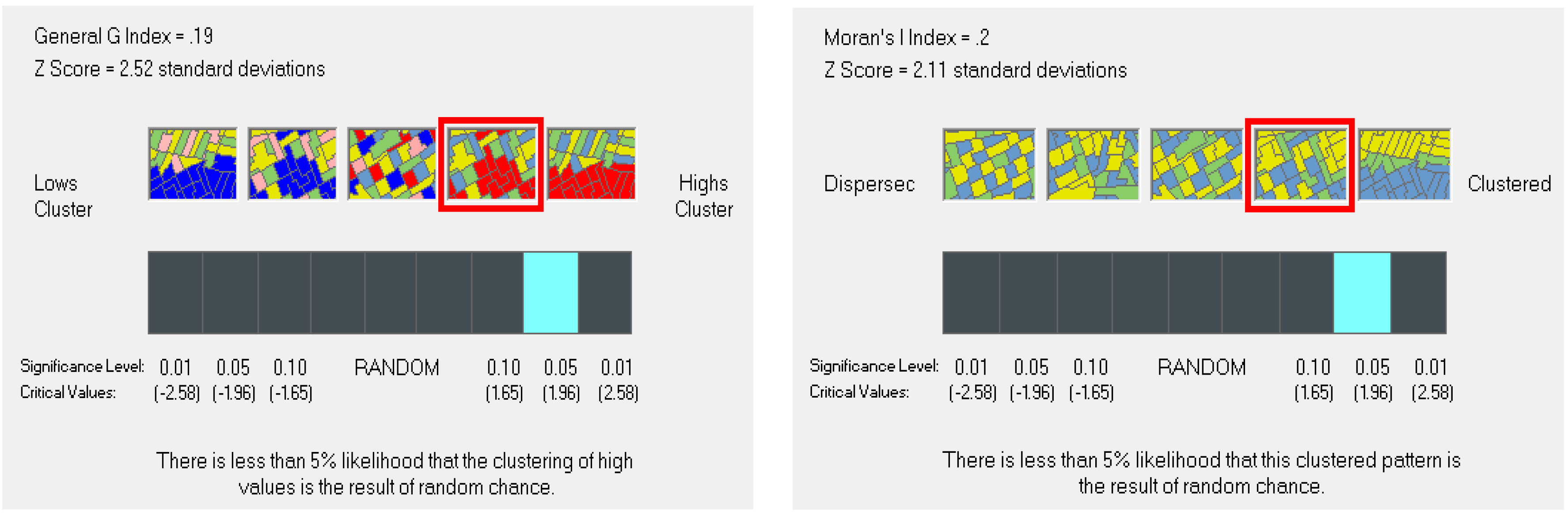
2.2.1. Global Spatial Autocorrelation

Global spatial autocorrelation can be used to measure the global correlation and disparity degree of some social economic phenomena. Statistic indices measuring global spatial autocorrelation include Moran’s I, Geary’s C and Getis’s G [20,24]. In this study, the Moran’s I and Getis’s G are used to measure global spatial autocorrelation of energy consumption change in China. Moran’s I can be expressed by the formula below:

(1)

where x_i is the observed value of certain attribute in the spatial unit i; x_j is the observed value of certain attribute in the spatial unit j; x is the mean value of regional variables; S² is the mean square deviation; W_ij is the spatial weight value, which is expressed by the n dimensional matrix W (n × n). The matrix is a standardized, which can be realized by spatial distance and topology.

The Getis’s G statistic of overall spatial association is given as:

(2)

where x_i and x_j are attribute values for features i and j, and w_{i, j} is the spatial weight between feature i and j.

The significance level of Moran’s I is commonly tested by the standardized Z_I-Score. Its equation is as follows:

(3)

where E (I) is the expected value of Moran’s I; and V (I) is the variance of Moran’s I.

The significance level of Getis’s G is commonly tested by the standardized Z_G-Score. Its equation is as follows:

(4)

where E (G) is the expected value of Getis’s G; and V (G) is the variance of Getis’s G.

The null hypothesis H₀ refers to the spatial correlation of energy consumption change do not exist. With a significance level of 0.05, if the absolute value of Z_I-Score or Z_G-Score is more than 1.96, the null hypothesis H₀ can be rejected. It is assumed that the n spatial attribute values are not spatially auto-correlated. It shows that significant correlation is observed between the variances.

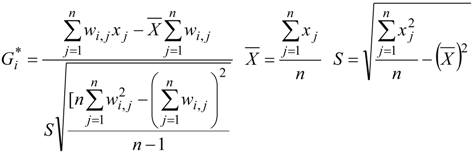
2.2.2. Local Spatial Autocorrelation

The local indicators of spatial association (LISA) are a series of indices decomposed directly by global spatial autocorrelation indicator. It is expressed by the distribution state of local heterogeneity and can be used to measure the spatial disparities degree between the regional i and its peri-regions. The Hot Spot Analysis tool calculates the Getis-Ord G_i^* statistic for each feature in a dataset. The resultant Z score tells you where features with either high or low values cluster spatially. This tool works by looking at each feature within the context of neighboring features. A feature with a high value is interesting, but may not be a statistically significant hot spot. To be a statistically significant hot spot, a feature will have a high value and be surrounded by other features with high values as well. The local sum for a feature and its neighbors is compared proportionally to the sum of all features; when the local sum is much different than the expected local sum, and that difference is too large to be the result of random chance, a statistically significant Z score results. The Getis-Ord local statistic G_i^* is given as:

(5)

where x_j is the attribute value for feature j, w_i,j is the spatial weight between feature i and j, n is equal to the total number of features.

The G_i^* statistic is a Z-score so no further calculations are required. The G_i^* statistic returned for each feature in the dataset is a Z score. For statistically significant positive Z scores, the larger the Z score is, the more intense the clustering of high values (hot spot). For statistically significant negative Z scores, the smaller the Z score is, the more intense the clustering of low values (cold spot).

Moran’s I scatter plot can visually reflect spatial autocorrelation [20]. Given certain significant level, we can obtain the LISA clustering map by combining the Moran’s I scatter plot. The LISA clustering plot can measure local spatial heterogeneous state and diagnosis hot spot and cold spot of spatial clustering about energy consumption change in the local space.

2.2.3. Spatial Autoregressive Model

According to the spatial correlations between the dependent variable and the independent variables, the most general formulation of the spatial autoregressive model is Equation (6) [22,24].

y = ρw₁y + xβ + ε
ε = λw₂ε + μ
μ ~ N(0, Ω)
Ω_ii = h_i (Zα), h_i > 0

(6)

where y is a (n × 1) vector representing the dependent variable, X is a (n × k) matrix representing the k − 1 independent variables, β is a (k × 1) vector of error terms presumed to have a covariance structure, ρ is the coefficients of spatial lag variable w₁y, ε is a (n × 1) vector of random error terms, W₂ is a (n × n) “weights” matrix reflecting the spatial trends of the residual, N is the normal distribution, Ω is the covariance matrix, Z is an exogenous variable, λ is the coefficient of spatial autoregressive structure w₂λ.

Based on the general formulation of the spatial autoregressive model, we can derive the spatial lag model and spatial error model. Spatial lag model takes into account the spatial correlation between dependent variables. The spatial lag model is Equation (7).

y = ρwy + xβ + μ

(7)

Spatial error model reflects the error process through the covariance of different. Spatial error model is Equation (8).

y = xβ + ε
ε = λwε + μ

(8)

Traditional goodness of fit index R² is not suitable for spatial regression model. Instead, a so-called goodness of fit index pseudo R² can be computed. In the spatial statistics, the pseudo R² is defined as the ratio of the variance of the predicted values over the variance of the observed values for the dependent variable [20,22]. In the standard regression model, unlike in the spatial lag model and spatial error model, this variance ratio is equivalent of the R² [20,22]. The goodness of fit indicators for spatial regression models based on maximum likelihood estimation include the Akaike Information Criterion (AIC), the maximized log likelihood (LIK) and the Schwartz Criterion [18]. The model with the lowest AIC, or with the highest LIK or with lowest SC has the best goodness-of-fit [19,23].

3. Results and Discussion

3.1. Analysis of Global Spatial Disparities

The GIS9.3 and OpenGeoDa softwares are used to conduct the exploratory spatial data analysis (ESDA) in this study. Based on the GIS9.3 and OpenGeoDa softwares, we have got the results about Global Moran’s I, Getis’s G and their statistic test of energy consumption change in China during the period 1990–2009 (see Figure 1 and Figure 2). From Figure 1, the Getis’s G or Global Moran’s I of energy consumption during the period 1990–2000 is 0.01, 0.24, respectively. The test of significance shows that the regional distribution of energy consumption change in China during the period 1990–2000 is significantly clustering (see Figure 1).

Figure 1. Getis’s G, Global Moran’s I and their statistic test of energy consumption change in China during the period 1990–2000.

Figure 1. Getis’s G, Global Moran’s I and their statistic test of energy consumption change in China during the period 1990–2000.

As can be seen from Figure 2, we conclude that the Getis’s G or Global Moran’s I of energy consumption during the period 2000–2010 is 0.19, 0.2, respectively. The test of significance also shows that regional distribution of energy consumption change in China during the period 1990–2010 is significantly clustering (see Figure 2).

Under the 95% confidence interval, the Moran’s I value of energy consumption in China is significantly positive from 1990 to 2010. This means that high and low energy consumption change in the research area is the same as that of its surrounding provinces. From Figure 1 and Figure 2, we can conclude that the global Moran’s I value decreased from 0.24 during the period 1990–2000 to 0.2 during the period 2000–2010, which means that the clustering trend of energy consumption change in China is weakened.

Figure 2. Getis’s G, Global Moran’s I and their statistic test of energy consumption change in China during the period 2000–2010.

Figure 2. Getis’s G, Global Moran’s I and their statistic test of energy consumption change in China during the period 2000–2010.

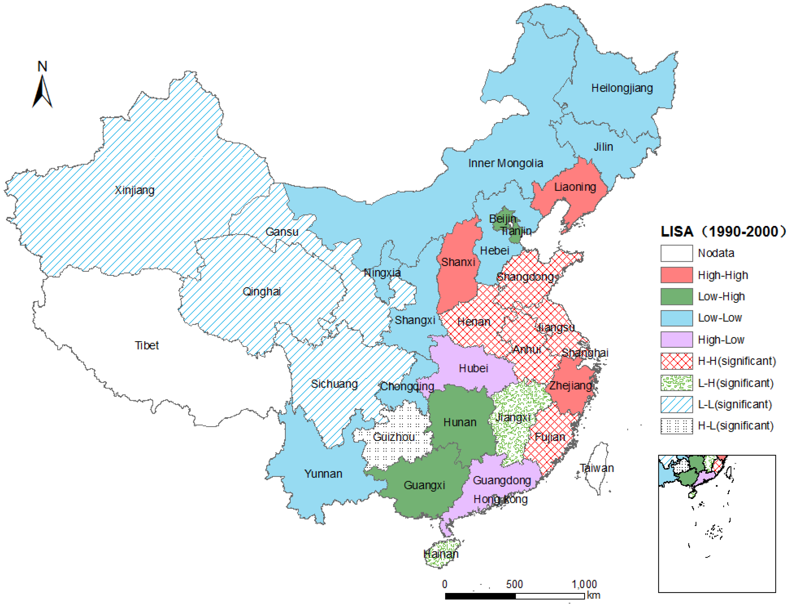
3.2. Analysis of Local Spatial Disparities

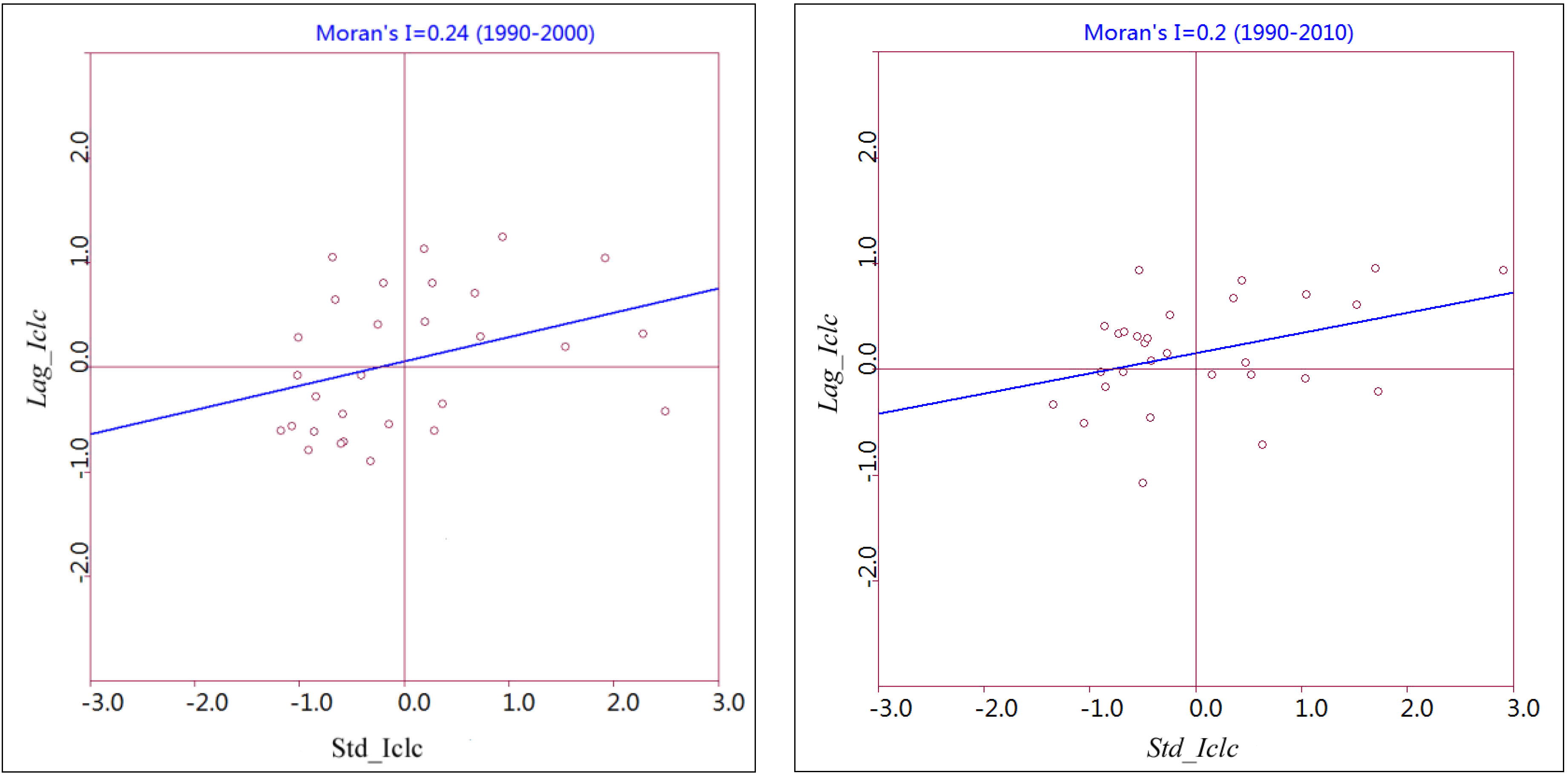
3.2.1. Analysis of Local Moran’s I_i

In order to explore the local spatial disparities of energy consumption change from 1990 to 2009 in China, we use the OpenGeoda software to obtain the results of local Moran’s I and its significant test during 1990–2000, during 2000–2010, and during 1990–2010 (see Table 1).

Table 1. Related parameters of local Moran’s I for energy consumption change in China from 1990 to 2010.

Time stage	Minimum	Maximum	Mean	Moran’s Ii (+)	Moran’s Ii (−)	Range
1990–2000	−1.0771	1.9914	0.2178	74.1935	25.8065	3.0685
2000–2010	−0.4994	2.7136	0.1822	51.6129	48.3871	3.2130
1990–2010	−0.5502	2.8206	0.2164	58.0650	41.9350	2.2704

Table 1. Related parameters of local Moran’s I for energy consumption change in China from 1990 to 2010.

Time stage	Minimum	Maximum	Mean	Moran’s Ii (+)	Moran’s Ii (−)	Range
1990–2000	−1.0771	1.9914	0.2178	74.1935	25.8065	3.0685
2000–2010	−0.4994	2.7136	0.1822	51.6129	48.3871	3.2130
1990–2010	−0.5502	2.8206	0.2164	58.0650	41.9350	2.2704

As can be seen from Table 1, the local Moran’s I value of each province in China is [−0.5502, 2.8206] during 1990–2010. The negative value of local Moran’s I shows that the spatial heterogeneity of energy consumption. Range of local Moran’s I value of each province in China is 3.0685 during 1990–2000. The maximum of local Moran’s I value is 1.9914 during 1990–2000 and 2.7136 during 1990–2000, which appeared in the Shandong Province. The minimum of local Moran’s I value is −1.0771 during 1990–2000 and located in the Guangdong Province. But the minimum of local Moran’s I value during 2000–2010 located in the Anhui Province. Table 1 also shows that there are significantly heterogeneous for energy consumption change during 1990–2010 and during 2000–2010 respectively. The changing rates of local Moran’s I value show the upward and downward trend respectively. From Table 1, we can also conclude that spatial aggregation of energy consumption change at province-level is weakened and spatial heterogeneity is enhanced.

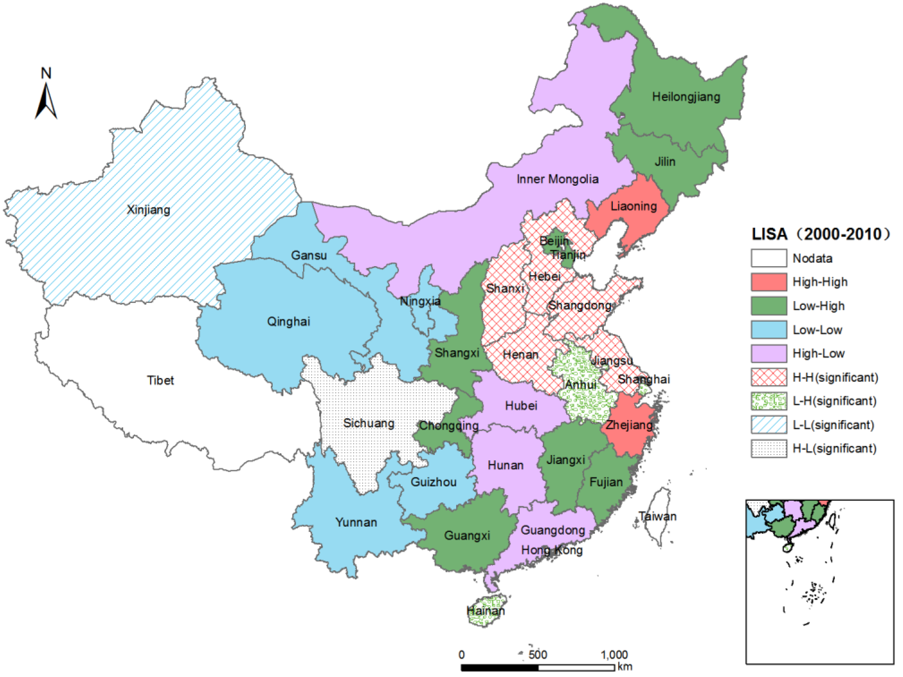
3.2.2. Analysis of Spatial Association Clustering and Distribution Features Based on Local Moran’s I_i

If variable Z and spatial variable W_z at each research unit are calculated to be used as the lateral axis and longitudinal axis, we can get the Moran scatter plot of energy consumption. In other words, standardized value (Std-I_clc) of research observation is used as the lateral axis, and spatial lagged value (Lag-I_clc) as the longitudinal axis. Moran scatter plot of energy consumption change is composed of local Moran’s I_i at each province in China (see Figure 3).

Figure 3. Moran scatter plot of energy consumption at province in China during 1990–2010.

Figure 3. Moran scatter plot of energy consumption at province in China during 1990–2010.

When the Std-I_clc value is positive in the Moran scatter plot, it means research unit belongs to those regions with faster energy consumption change. Otherwise it belongs to those areas with slow energy consumption changes. Those areas with positive Std-I_clc value account for 40% at the whole time stage (see Table 2). Those areas with positive Std-I_clc value is both 40% during 1990–2000 and during 2000–2010 and, which means that there is no change about the number of those areas with faster energy consumption change in the view of spatial association at the whole time stage. The Lag-I_clc value is positive in the Moran scatter plot, which means surrounding regions of research unit belonged to those regions with faster energy consumption change. While the number of those areas with positive Lag-I_clc value remains 63% at the whole time stage, the number of those regions with positive Lag-I_clc value increased from 50% during 1990–2000 to 63% during 2000–2010, which means a number of surrounding regions of research unit with faster energy consumption change increased in the view of spatial association.

According to the composite attribute of the Std-I_clc index and Lag-I_clc one, four area types of energy consumption change were divided by positive or negative spatial association (see Table 2). The four area types are High–High type of positive correlation (H–H), Low-Low type of positive correlation (L–L), Low-High type of negative correlation (L–H) and High-Low type of negative correlation (H–L).

As can be seen from Table 2, those regions belonging to High-High type account for 40% during the period 1990–2010, which include Jiangsu Province, Hebei Province and Shandong Province, where there is rapid development of urbanization and industrialization, and regions belonging to Low–Low type account for 30% during 1990–2010, which include Qinghai Province, Xinjiang Province and Ningxia Province with the slow development of urbanization and industrialization.

Table 2. Related parameters and disparities type of standardized variable Z for energy consumption change at province level in China (%).

Time Stage	Std-Iclc > 0	Std-Iclc < 0	Lag-Iclc > 0	Lag-Iclc < 0	H–H		H–L		L–L		L–H
	Ratio	Ratio	Ratio	Ratio	Comparison Ratio	Ratio	Comparison Ratio	Ratio	Comparison Ratio	Ratio	Comparison Ratio	Ratio
1990–2000	40.00	60.00	50.00	50.00	S+L+	30.00	S+L−	10.00	S−L−	26.67	S−L+	23.33
2000–2010	40.00	60.00	63.33	36.67	S+L+	23.33	S+L−	16.67	S−L−	16.67	S−L+	33.33
1990–2010	40.00	60.00	63.33	36.67	S+L+	23.33	S+L−	16.67	S−L−	30.00	S−L+	30.00

Notes: S₊—Std-I_clc > 0, S₋—Std-I_clc < 0, L₊—Lag-I_clc > 0, L₋—Lag-I_cl.

Table 2. Related parameters and disparities type of standardized variable Z for energy consumption change at province level in China (%).

Time Stage	Std-Iclc > 0	Std-Iclc < 0	Lag-Iclc > 0	Lag-Iclc < 0	H–H		H–L		L–L		L–H
	Ratio	Ratio	Ratio	Ratio	Comparison Ratio	Ratio	Comparison Ratio	Ratio	Comparison Ratio	Ratio	Comparison Ratio	Ratio
1990–2000	40.00	60.00	50.00	50.00	S+L+	30.00	S+L−	10.00	S−L−	26.67	S−L+	23.33
2000–2010	40.00	60.00	63.33	36.67	S+L+	23.33	S+L−	16.67	S−L−	16.67	S−L+	33.33
1990–2010	40.00	60.00	63.33	36.67	S+L+	23.33	S+L−	16.67	S−L−	30.00	S−L+	30.00

Notes: S₊—Std-I_clc > 0, S₋—Std-I_clc < 0, L₊—Lag-I_clc > 0, L₋—Lag-I_cl.

In order to effectively explore more spatial characteristics of energy consumption change in China during 1990–2010, LISA clustering map of two time stages were formed by matching the proper type to corresponding spatial location of each province during 1990–2000 and during 2000–2010 (see Figure 4 and Figure 5).

From Figure 4 and Figure 5, we conclude that the regions belonging to H–H type have positive spatial autocorrelation, where Std-I_clc > 0 and Lag-I_clc > 0. This indicates the local spatial disparities of energy consumption change are smaller and stronger for local homogeneity in the research unit while the changes of energy consumption in their surrounding units are relatively higher. Table 2 shows that the proportion of those regions, which are located in the coastal area with high-level economic development in China, decreased from 30% during 1990–2000 to 23% during 2000–2010. Among them, Jiangsu Province plays a significant role during the two periods. The higher standard of economic development and industrialization in those regions are the main causes for higher energy consumption changes.

Figure 4 and Figure 5 also show that those regions belonging to L–L type have also positive spatial autocorrelation, where Std-I_clc < 0 and Lag-I_clc < 0. This means that the local spatial disparities of energy consumption change are smaller and stronger in local homogeneity in the research units and relatively slow in their surrounding units. The number of those type regions decreased from 12 during 1999–2000 to 8 during 2000–2010. The ratio of energy consumption change in L–L type area is lower than average. 26.67% type region is lower than average level during 1999–2000. All provinces are significantly distributed in the north-western regions with low-level development of economy in China. Xinjiang Province particularly, has significantly positive relationship during 1990–2009 and during 2000–2010.

The regions belonging to the L–H type have a negative spatial autocorrelation, where Std-I_clc < 0 and Lag-I_clc > 0 (see Figure 4 and Figure 5). This means that local spatial disparities of energy consumption change are smaller in local heterogeneity in the research unit and higher in their surrounding units. Energy consumption changes in the research unit are relatively slow, which forms a cold spot of the local heterogeneity. The number in the L-H type is 6 during 1990–2000 and 12 during 2000–2010. Those regions are significantly located in Jiangxi Province and Hainan Province during 1990–2000 and during 2000–2010. Anhui province forms a cold spot of the local heterogeneity due to the higher energy consumption in its surrounding provinces including Zhejiang province, Jiangsu province and Shandong province.

Figure 4. LISA clustering of energy consumption change in China during the period 1990–2000.

Figure 4. LISA clustering of energy consumption change in China during the period 1990–2000.

Figure 5. LISA clustering of energy consumption change in China during the period 2000–2010.

Figure 5. LISA clustering of energy consumption change in China during the period 2000–2010.

The regions belonging to the H–L type have a negative spatial autocorrelation, where Std-I_clc > 0 and Lag-I_clc < 0. This means that the local spatial disparities of energy consumption change are larger and stronger in local heterogeneity in the research unit and slower in their surrounding units. Energy consumption changes in the research unit are relatively slow, which forms a hot spot of the local heterogeneity. The ratio of energy consumption changes in the H–L type is higher than average. The number in the H–L type is 3 during 1990–2000 and 5 during 2000–2010.

3.3. Influencing Factors of Energy Consumption Change

Studies show that energy demand is dominated by the level of economic development, pricing, change of industry structure, population growth, technological progress, the level of urbanization and other factors [12,14]. General empirical studies usually assume energy consumption and energy demand are equal [12,14]. In order to explore the influencing factors of energy consumption change during 2000–2009 in China, six independent variables were selected into the standard regression model. Before conducting the regression analysis, we made a preliminary diagnosis between independent variables. The coefficient of determination R² between the independent variables is in the range of 0.12 to 0.71, lower than the critical value of 0.8 [30]. Therefore, all the independent variables can be incorporated into the regression model.

Moran’s I values and the results of their statistic test of six independent variables in the regression model are listed in Table 3. As can be seen from Table 3, all the variables, except the independent variables Industrialized rate, have demonstrated a significantly positive spatial autocorrelation. This indicates that the driving forces of China’s energy consumption changes also showed a positively spatial autocorrelation. Among them, the significance levels of independent variable GDP growth rate and percentage of transportation industry production value change are the largest. Therefore, the spatial spillover of independent variables should be considered in analyzing the influencing factors of energy consumption in China.

Table 3. Moran’s I values and their statistic test of independent variables of regression model.

Independent Variable	Moran’s I	E (I)	Mean	SD	ZI-score
Population growth rate	0.3476 *	−0.0345	−0.0326	0.1127	3.3904
GDP growth rate	0.4580 **	−0.0345	−0.0363	0.1160	4.2456
Urbanization rate	0.3781 *	−0.0345	−0.0319	0.1145	3.6035
Industrialized rate	0.0022	−0.0345	−0.0264	0.1133	0.3239
Percentage of industry production value change	0.2073 *	−0.0345	−0.0302	0.0997	2.4252
Percentage of transportation industry production value change	0.4439 **	−0.0345	−0.0337	0.1135	4.2149

* p < 0.05, ** p < 0.001.

Table 3. Moran’s I values and their statistic test of independent variables of regression model.

Independent Variable	Moran’s I	E (I)	Mean	SD	ZI-score
Population growth rate	0.3476 *	−0.0345	−0.0326	0.1127	3.3904
GDP growth rate	0.4580 **	−0.0345	−0.0363	0.1160	4.2456
Urbanization rate	0.3781 *	−0.0345	−0.0319	0.1145	3.6035
Industrialized rate	0.0022	−0.0345	−0.0264	0.1133	0.3239
Percentage of industry production value change	0.2073 *	−0.0345	−0.0302	0.0997	2.4252
Percentage of transportation industry production value change	0.4439 **	−0.0345	−0.0337	0.1135	4.2149

* p < 0.05, ** p < 0.001.

The Akaike Information Criterion (AIC), maximized log likelihood (LIK) and Schwartz Criterion [18] are given for the comparison with three spatial models. The LIK of the spatial lag model is higher than the LIK of standard linear model and spatial error model (see Table 4). The spatial lag model (SLM) has the best goodness-of-fit compared with the other two models because of its lowest AIC, highest LIK, or lowest SC (Table 4). At the significant level (p < 0.05), the spatial lag model has passed the Likelihood Ratio Test. Thus, the spatial lag model (SLM) is better than the linear regression model and the spatial error model (SEM) for analyzing the factors that affect energy consumption in China.

The results of three regression models for energy consumption change in China during 2000–2010 are listed in Table 5. The output results contain the goodness-of-fit (R² or Pseudo R²), estimated coefficient, standard error, t-test value or z-test value and associated probability. As can be seen from Table 5, almost all the independent variables in the spatial lag model were tested significance level (p < 0.05), indicating that the spatial lag model is superior to spatial error model.

Table 4. Statistical tests of three regression models.

Model type	R2 or Pseudo R2	LIK	AIC	SC
Linear regression model	0.8065	3.7631	6.4737	16.5117
Spatial lag model (SLM)	0.8425	6.5164	2.9673	14.4392
Spatial error model (SEM)	0.8075	3.7948	6.4103	16.4482

Table 4. Statistical tests of three regression models.

Model type	R2 or Pseudo R2	LIK	AIC	SC
Linear regression model	0.8065	3.7631	6.4737	16.5117
Spatial lag model (SLM)	0.8425	6.5164	2.9673	14.4392
Spatial error model (SEM)	0.8075	3.7948	6.4103	16.4482

Compared with the significance level of the parameters for three models, this study concludes that significance level of the parameters increases, and that six variables—Population growth rate, GDP growth rate, Urbanization rate, Industrialized rate, Percentage of industry production value change, Percentage of transportation industry production value change—have significantly correlated with energy consumption change in the spatial lag model (p < 0.05).

From Table 5, we conclude that the variable Population growth rate has a strongly positive relation with energy consumption change in three regression models, which means that those areas with higher population growth rate have significantly higher growth of energy consumption. Population growth is one of the traditional factors that determine energy demand [12], this conclusion is also shown in Table 5. The higher the rate of population growth will increase the demand for energy consumption. In recent years, with the continuous improvement of the public’s income and living standards, the living energy consumption will grow along with the steady growth of population and per capita energy consumption will continue to rise.

At the 0.05% significance level, Table 5 also shows that the variable GDP growth rate has all strongly positive relation with energy consumption change in three regression models. This means the higher regional economic development level is, the larger the energy consumption change would be. The result proves the above conclusion based on the analysis of local Moran’s I_i. Related studies have shown that economic growth and its impact on quality of life are major factors in promoting the growth of energy consumption [14]. Our study also supports this conclusion.

The variable Urbanization rate has strongly negative relation with energy consumption in the spatial lag model (see Table 5). This means that those areas with higher urbanization have significantly lower energy consumption. This may be because higher urbanized areas pay more attention to the impact of efficiency and technological progress on energy consumption.

From Table 5 (B), we can conclude that the variable Industrialized rate has a strong positive relation with energy consumption change in the spatial lag model, which means that those areas with higher industrialization have significantly larger energy consumption. The variable Industrialized rate reflects the impacts of industrial structure on energy consumption. According to the evolution characteristics of China’s regional economic development stage, the industrial structure is another important factor affecting energy consumption demand, especially in the second industrial industry. Due to the characteristics of the industry itself, the intensity of its energy consumption is much higher than other industries.

Table 5. Parameters of three different regression models for energy consumption change in China during 2000–2010.

Variable	Coefficient	Std. Error	t Statistic	Probability
(A) Linear regression model R2 = 0.8065
Constant	0.0251	0.2425	0.1034	0.9185
Population growth rate	0.3109	0.0826	3.7640	0.0010
GDP growth rate	0.6732	0.2250	2.9924	0.0063
Urbanization rate	−1.1445	0.2193	−5.2181	0.0000
Industrialized rate	0.3300	0.2028	1.6269	0.1168
Percentage of industry production value change	0.1439	0.0805	1.7887	0.0863
Percentage of transportation industry production value change	0.3321	0.1804	1.8407	0.0781
Variable	Coefficient	Std. Error	Z-value	Probability
(B) Spatial lag model Pseudo R2 = 0.8425
ρ	−0.3713	0.1427	−2.6011	0.0093
Constant	0.1942	0.2002	0.9700	0.3321
Population growth rate	0.3268	0.0656	4.9787	0.0000
GDP growth rate	0.7766	0.1814	4.2811	0.0000
Urbanization rate	−1.2822	0.1779	−7.2057	0.0000
Industrialized rate	0.3868	0.1628	2.3763	0.0175
Percentage of industry production value change	0.1783	0.0654	2.7268	0.0064
Percentage of transportation industry production value change	0.4302	0.1446	2.9745	0.0029
Variable	Coefficient	Std. Error	Z-value	Probability
(C) Spatial error model Pseudo R2 = 0.8075
λ	−0.1227	0.2709	−0.4529	0.6506
Constant	0.0557	0.2122	0.2624	0.7930
Population growth rate	0.3094	0.0723	4.2819	0.0000
GDP growth rate	0.6730	0.1960	3.4345	0.0006
Urbanization rate	−1.1609	0.1941	−5.9822	0.0000
Industrialized rate	0.3287	0.1796	1.8297	0.0673
Percentage of industry production value change	0.1423	0.0701	2.0294	0.0424
Percentage of transportation industry production value change	0.3623	0.1589	2.2793	0.0226

Table 5. Parameters of three different regression models for energy consumption change in China during 2000–2010.

Variable	Coefficient	Std. Error	t Statistic	Probability
(A) Linear regression model R2 = 0.8065
Constant	0.0251	0.2425	0.1034	0.9185
Population growth rate	0.3109	0.0826	3.7640	0.0010
GDP growth rate	0.6732	0.2250	2.9924	0.0063
Urbanization rate	−1.1445	0.2193	−5.2181	0.0000
Industrialized rate	0.3300	0.2028	1.6269	0.1168
Percentage of industry production value change	0.1439	0.0805	1.7887	0.0863
Percentage of transportation industry production value change	0.3321	0.1804	1.8407	0.0781
Variable	Coefficient	Std. Error	Z-value	Probability
(B) Spatial lag model Pseudo R2 = 0.8425
ρ	−0.3713	0.1427	−2.6011	0.0093
Constant	0.1942	0.2002	0.9700	0.3321
Population growth rate	0.3268	0.0656	4.9787	0.0000
GDP growth rate	0.7766	0.1814	4.2811	0.0000
Urbanization rate	−1.2822	0.1779	−7.2057	0.0000
Industrialized rate	0.3868	0.1628	2.3763	0.0175
Percentage of industry production value change	0.1783	0.0654	2.7268	0.0064
Percentage of transportation industry production value change	0.4302	0.1446	2.9745	0.0029
Variable	Coefficient	Std. Error	Z-value	Probability
(C) Spatial error model Pseudo R2 = 0.8075
λ	−0.1227	0.2709	−0.4529	0.6506
Constant	0.0557	0.2122	0.2624	0.7930
Population growth rate	0.3094	0.0723	4.2819	0.0000
GDP growth rate	0.6730	0.1960	3.4345	0.0006
Urbanization rate	−1.1609	0.1941	−5.9822	0.0000
Industrialized rate	0.3287	0.1796	1.8297	0.0673
Percentage of industry production value change	0.1423	0.0701	2.0294	0.0424
Percentage of transportation industry production value change	0.3623	0.1589	2.2793	0.0226

From Table 5 (B), we conclude that the most influencing factor is the variable Percentage of industry production value change, which is mainly induced by transportation industry. On the one hand, change of vehicle fuel consumption is main driver forces of energy consumption change in China during 2000–2010. On the other hand, the material flows and energy flows between regions linked by transportation industry. The increase in the significance levels of the variable Percentage of industry production value change in the spatial lag model and spatial error model shows the spatial spillover of transportation industry is obvious.

In this study, when the influencing factors of energy consumption changes in China were analyzed by using the classical linear regression model, the effects of spatial autocorrelation were ignored. The spatial regression model provides a statistically reasonable solution. Compared to the classical linear regression model, there is no spatial autocorrelation of the residuals in the spatial error model, and it has a better goodness-of-fit. All the independent variables were tested significance level (p < 0.05) in the spatial error model, which can reveal more influencing factors of energy consumption changes in China.

This study did not consider the impact of energy consumption structure and price on the energy consumption changes. In future studies, we should pay attention to the impact of energy consumption structure on global climate change due to coal and gas has different implications in terms of global Climate Change. It should also be focused on the effecting mechanism of energy prices on energy consumption in our future research work.

4. Conclusions

Traditional methods measuring the regional disparities ignored the factor of geographical position, which may not truly reflect the spatial characteristics of regional disparities. ESDA mainly measuring spatial association can solve the problem of spatial relationship between regions. It provides the stronger support for the quantitative analysis of spatial disparities of energy consumption change.

Energy consumption changes in China and its driving forces have shown a spatially positive correlation. The residuals of standard regression model also showed positive autocorrelation, indicating that stand multiple linear regression model failed to consider all the spatial dependencies.

The regional distribution of energy consumption change has significant clustering characteristics during 1990–2010 in China. This means that energy consumption change of research unit and its surrounding areas are higher.

Based on the composite attribute of Std-I_clc value and Lag-I_clc value, Moran’s scatter divides into four type regions and two spatial associations. Because the characteristics, causes and spatial disparities of energy consumption change in the four type regions are different, the strategies and measures of energy consumption should be put forward for each clustering regions in China.

The results of spatial autoregressive model show that higher industrialization rate and economic development level are the main causes for higher energy consumption change.

According to the conclusions of regression analysis, this study has proposed the following measures to deal with the growing trend of energy consumption changes in China. Firstly, during the process of China’s rapid urbanization, we should establish diversified energy consumption patterns, and improve the quality of the energy use. Secondly, in China’s economically developed eastern provinces, we should optimize the industrial structure and reduce the proportion of energy-intensive industries. Thirdly, governments need to actively promote the public transport system, reducing the proportion of energy consumption in the transportation sector. Energy demand in various regions of China will continue to grow in the coming periods, especially the energy consumption of second industrial, which is the most important factor in China’s energy consumption. The emphasis should be placed on energy policy in China to reduce the proportion of secondary industry in the national economy structure by optimizing adjustment, especially thereby improving industrial energy efficiency through technological innovation and other aspects. Second, insisting on population control policy will curb faster growth trend of energy demand to some extent. The transformation of economic growth mode and the regulation of the price mechanism in the area of energy demand are imperative. Meanwhile, the government should develop the spatial differentiated policies and measures of energy supply and demand. This study also shows that it needs to focus on the important role of geospatial factors in the area of adjustment localization policy for energy consumption behavior.

This article also shows that ESDA and spatial autoregressive model of spatial statistics are some effective methods to measure the spatial pattern and main driving forces of energy consumption change and to explore the distribution characteristics, local heterogeneity and homogeneity of many spatial social-economical phenomena by the comparison with general clustering analysis. This study also indicate that the spatial auto-regression model can reveal more influencing factors of energy consumption changes in China, in contrast with standard linear model.

References

1. Arouri, M.E.; Ben Youssef, A.; M’Henni, H.; Rault, C. Energy consumption, economic growth and CO2 emissions in Middle East and North African countries. Energy Policy 2012, 45, 342–349. [Google Scholar] [CrossRef] [Green Version]
2. Payne, J.E. The Causal Dynamics Between US Renewable Energy Consumption, Output, Emissions, and Oil Prices. Energy Sour. Part B—Econ. Plan. Policy 2012, 7, 323–330. [Google Scholar] [CrossRef]
3. Deng, S.H.; Zhang, J.; Shen, F.; Guo, H.; Li, Y.W.; Xiao, H. The Relationship Between Industry Structure, Household-number and Energy Consumption in China. Energy Sour. Part B-Econ. Plan. Policy 2014, 9, 325–333. [Google Scholar] [CrossRef]
4. Dong, X.B.; Ulgiati, S.; Yan, M.C.; Zhang, X.S.; Gao, W.S. Energy and eMergy evaluation of bioethanol production from wheat in Henan Province, China. Energy Policy 2008, 36, 3882–3892. [Google Scholar] [CrossRef]
5. Dong, X.B.; Zhang, Y.F.; Cui, W.J.; Xun, B.; Yu, B.H.; Ulgiati, S.; Zhang, X.S. Emergy-Based Adjustment of the Agricultural Structure in a Low-Carbon Economy in Manas County of China. Energies 2011, 4, 1428–1442. [Google Scholar] [CrossRef]
6. Liu, Y.B. Exploring the relationship between urbanization and energy consumption in China using ARDL (autoregressive distributed lag) and FDM (factor decomposition model). Energy 2009, 34, 1846–1854. [Google Scholar] [CrossRef]
7. Liu, Y.B.; Xie, Y.C. Asymmetric adjustment of the dynamic relationship between energy intensity and urbanization in China. Energy Econ. 2013, 36, 43–54. [Google Scholar] [CrossRef]
8. Lu, W.W.; Chen, C.; Su, M.R.; Chen, B.; Cai, Y.P.; Xing, T. Urban energy consumption and related carbon emission estimation: A study at the sector scale. Front. Earth Sci. 2013, 7, 480–486. [Google Scholar] [CrossRef]
9. Yu, H.Y. The influential factors of China’s regional energy intensity and its spatial linkages: 1988–2007. Energy Policy 2012, 45, 583–593. [Google Scholar] [CrossRef]
10. Liu, Y.B. Energy Production and Regional Economic Growth in China: A More Comprehensive Analysis Using a Panel Model. Energies 2013, 6, 1409–1420. [Google Scholar] [CrossRef]
11. Dietz, T.; Stern, P.C.; Weber, E.U. Reducing Carbon-Based Energy Consumption through Changes in Household Behavior. Daedalus 2013, 142, 78–89. [Google Scholar] [CrossRef]
12. Wu, Y. Determinants and Spatial Spillovers Effects of Regional Energy Consumption in China: Positive Study Based on Spatial Panel Data Econometric Models. J. Nanjing Agric. Univ. 2012, 12, 124–132. [Google Scholar]
13. Zou, Y.; Lu, Y. Regional characteristics of energy efficiency in China based on spatial auto regression model. Stat. Res. 2005, 10, 67–71. [Google Scholar]
14. Wang, H.G.; Shen, L.S. A Spatial Panel Statistical Analysis on Chinese Economic Growth and Energy Consumption. J. Quant. Tech. Econ. 2007, 12, 98–107. [Google Scholar]
15. Wu, Y.; Li, J. A local spatial econometric study on relationship between electricity consumption and economic growth of Chinese provinces. Sci. Geogr. Sin. 2009, 29, 30–35. [Google Scholar]
16. Guo, L.; Du, S.H.; Haining, R.; Zhang, L.J. Global and local indicators of spatial association between points and polygons: A study of land use change. Int. J. Appl. Earth Obs. 2013, 21, 384–396. [Google Scholar] [CrossRef]
17. Ertur, C.; Koch, W. Regional disparities in the European Union and the enlargement process: An exploratory spatial data analysis, 1995–2000. Ann. Reg. Sci. 2006, 40, 723–765. [Google Scholar] [CrossRef]
18. Ruiz, A.R.; Pascual, U.; Romero, M. An exploratory spatial analysis of illegal coca cultivation in Colombia using local indicators of spatial association and socioecological variables. Ecol. Indic. 2013, 34, 103–112. [Google Scholar] [CrossRef]
19. Anselin, L.; Sridharan, S.; Gholston, S. Using exploratory spatial data analysis to leverage social indicator databases: The discovery of interesting patterns. Soc. Indic. Res. 2007, 82, 287–309. [Google Scholar] [CrossRef]
20. Anselin, L. Spatial Econometrics: Methods and Models; Kluwer Academic Publishers: Dordrecht, The Netherlands, 1988. [Google Scholar]
21. Xie, H.L.; Liu, Z.F.; Wang, P.; Liu, G.Y.; Lu, F.C. Exploring the Mechanisms of Ecological Land Change Based on the Spatial Autoregressive Model: A Case Study of the Poyang Lake Eco-Economic Zone, China. Int. J. Environ. Res. Public Health 2013, 11, 583–599. [Google Scholar] [CrossRef]
22. Anselin, L. Local indicators of spatial association. Geogr. Anal. 1995, 27, 93–115. [Google Scholar] [CrossRef]
23. Anselin, L. From SpaceStat to CyberGIS: Twenty Years of Spatial Data Analysis Software. Int. Reg. Sci. Rev. 2012, 35, 131–157. [Google Scholar] [CrossRef]
24. Getis, A.; Ord, K. The analysis of spatial association by use of distance statistics. Geogr. Anal. 1992, 24, 189–206. [Google Scholar] [CrossRef]
25. Poulsen, M.; Johnston, R.; Forrest, J. The intensity of ethnic residential clustering: Exploring scale effects using local indicators of spatial association. Environ. Plan. A 2010, 42, 874–894. [Google Scholar] [CrossRef]
26. Gray, D. District House Price Movements in England and Wales 1997–2007: An Exploratory Spatial Data Analysis Approach. Urban Stud. 2012, 49, 1411–1434. [Google Scholar] [CrossRef]
27. Gaither, C.J.; Poudyal, N.C.; Goodrick, S.; Bowker, J.M.; Malone, S.; Gan, J.B. Wildland fire risk and social vulnerability in the Southeastern United States: An exploratory spatial data analysis approach. For. Policy Econ. 2011, 13, 24–36. [Google Scholar] [CrossRef]
28. Xie, H.L.; Wang, P.; Huang, H.S. Ecological Risk Assessment of Land Use Change in the Poyang Lake Eco-economic Zone, China. Int. J. Environ. Res. Public Health 2013, 10, 328–346. [Google Scholar] [CrossRef]
29. Xie, H.L.; Kung, C.C.; Zhao, Y.L. Spatial disparities of regional forest land change based on ESDA and GIS at the county level in Beijing-Tianjin-Hebei area. Front. Earth Sci. 2012, 6, 445–452. [Google Scholar] [CrossRef]
30. Menard, S. Applied Logistic Regression Analysis; Sage: Thousand Oaks, CA, USA, 1995. [Google Scholar]