1. Introduction
The computable general equilibrium (CGE) model provides a consistent framework to analyze the economic impacts of energy and environmental policy. It has sound micro-economic foundations and a complete description of the economy with both direct and indirect effects of policy changes. Since the 1980s, the CGE model has been more widely applied and became the mainstream of energy and environmental policy analysis.
Many developed CGE models, researching energy and environmental policy, are static (Akkemik and Oguz [
1], Xie and Saltzman [
2], Fraser and Waschik [
3], Caron [
4], Boccanfuso
et al. [
5]). Interest for forecast and analysis of trends has triggered the flourish of dynamic CGE models. Thus, there are growing numbers of literatur on dynamic CGE models for energy and environmental problems. Vennemo [
6] discussed the nature of environmental feedbacks on the Norwegian economy by using the general equilibrium model DREAM (Dynamic Resource/Environment Applied Model). Wendner [
7] analyzed environmental tax reforms, which use the revenues from CO
2 taxation to partially finance the pension system within the framework of a dynamic computable general equilibrium model (DCGE). By using this DCGE model, Muto
et al. [
8] simulated the automobile and the related carbon tax needed to accomplish the objective in the transport sector in Japan. Fukiharu [
9] used the dynamic general equilibrium approach to examine the effect of the greenhouse effect on the sustainability of human population, as well as the economic policies when the sustainability is in danger. By establishing a single-country (Japan) dynamic computable general equilibrium model with endogenous technological change, Matsumoto [
10] evaluated the economic and environmental effects of climate change mitigation in a country scale considering various time horizons in the analysis. O’Ryan
et al. [
11] developed a dynamic CGE model for Chile and made a quantitative analysis of the socioeconomic and environmental impacts of different trade agreements. This study aimed to compare the consequences of unilateral liberalization and trade agreements from Chile with the performance from European Union (EU) and the United States (USA). Hermeling
et al. [
12] introduced a new method for stochastic sensitivity analysis for CGE model, based on Gauss Quadrature, and applied it to check the robustness of a large-scale climate policy evaluation before making an impact assessment of EU2020 climate policy.
Meantime, several energy and environment related studies with static CGE models can be found in China. He
et al. [
13] analyzed the influence of coal price adjustment on the electric power industry, and the influence of electricity price adjustment on the macroeconomy in China, based on a static CGE models. Lin and Jiang [
14] applied the price-gap approach to estimate China’s energy subsidies and analyzed the economic impacts of energy subsidy reforms in China through a CGE model. The results showed that removing energy subsidies will result in a significant fall in energy demand and emissions, but will impact the macroeconomic variables negatively (See other relevant studies, such as Ren
et al. [
15], He
et al. [
16], Lu
et al. [
17], and Zhang
et al. [
18]).
Furthermore, some dynamic CGE models have also been proposed to assess the energy and environment problems in China. Zhang [
19,
20] analyzed the macroeconomic effects of limiting China’s CO
2 emissions by using a time-recursive dynamic CGE model of the Chinese economy. The baseline scenario for Chinese economy over the period to 2010 is first developed under a set of assumptions about the exogenous variables. Garbaccio
et al. [
21] built a recursive dynamic CGE model and evaluated the impacts of carbon tax on the economy of China, whilst considering the coexistence of planned economy and market economy. Liang
et al. [
22] established a dynamic CGE model to simulate a carbon tax policy in China, and compared the macroeconomic effects of different carbon tax schemes as well as their impacts on the energy- and trade-intensive sectors. By constructing a dynamic recursive general equilibrium model, Lu
et al. [
23] explored the impact of carbon tax on Chinese economy, as well as the cushion effects of the complementary policies. Recently, based on a multi-sector dynamic CGE model, Tang
et al. [
24] examined the impacts of the proposed carbon-based border tax adjustments (BTAs) with different tax rates from $20 to $100 per ton of carbon emissions (tC) imposed by both USA and EU on China’s international trade. The simulation results suggested that BTAs would have a negative impact on China’s international trade, incurring large losses in both exports and imports.
Dynamic models obviously incorporate the accumulation processes of an economy (in particular, investment), and increase the mid/long term predictive capability of the simulations. Nevertheless, they also increase the complexity of the assessment by adding the trends of the economic variables to the inter-relations in a specific moment of time. In addition, the CGE model is more suitable for the counties and regions in which market economy system is relatively perfect. However, China is in a specific period of transition from a planned to a market economy, and the market equilibrium mechanism is not perfect. In this case, the simulation results of a dynamic CGE model may be quite different from the actual situation. When we plan to set a dynamic CGE model, it requires us to set the relevant parameters of dynamic scene as reasonable as possible to make sure the dynamic simulation results are in accordance with the objective reality of China’s economic development.
Therefore, this paper intends to develop a dynamic CGE model to study the development trend and the changing characteristics of economy, energies’ consumption and carbon emissions from 2007 to 2030, as well as to analyze the impact of carbon tax policy and clean energy technology progress on economy, energies’ consumption, and carbon emission.
This paper is organized as follows:
Section 2 introduces the model structures and functions characteristics.
Section 3 discusses how to divide the sectors, especially the energies sectors by the RAS (Bi-proportional Scaling Method) method.
Section 4 depicts the detailed calculation and handling process of carbon emissions coefficients, and the setting of dynamic benchmark scenario parameters.
Section 5 analyzes the variation characteristics of China’s gross domestic product, the total energy consumption, energy consumption intensity, carbon emissions, and carbon emissions intensity under the benchmark scenario.
Section 6 studies the effects on GDP, energy consumption and carbon emissions under different scenarios of carbon tax policy. Finally, conclusions and suggestions are proposed in
Section 7, based on the comprehensive analysis presented in
Section 5 and
Section 6.
2. Theoretical Framework of the CGE Model for China
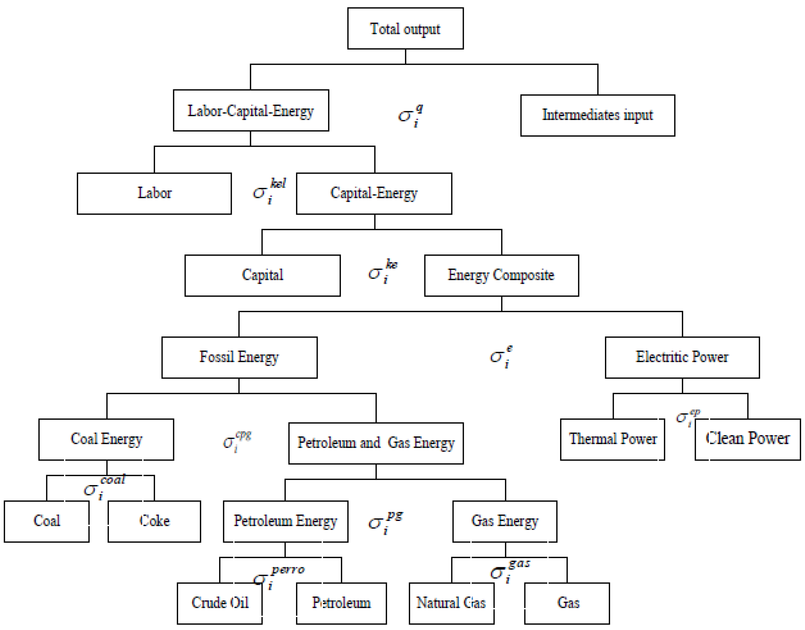
2.1. Production Module
Production functions for each sector describe the ways in which capital, labor, energy, and intermediate inputs can be used to produce output. Overall, the production process is represented by a seven-layer nested Constant Elasticity of Substitution (CES) function (
i.e., constant elasticity of substitute function) as depicted in
Figure 1 (where is the elasticity of substitute). The top layer of the nest structure comprises the composite primary inputs of labor, capital, and energy, as well as intermediate inputs. Following Burniaux
et al. [
25] and Huang
et al. [
26], we assume that the relationship between energy and capital is quasi-complementary, while the substitute elasticity between capital/energy and labor is larger. Therefore, the second layer determines the producer’s demand for input of labor and the composite capital and energy. At the third layer, the composite capital and energy is disaggregated into capital and energy. As electricity is mainly generated by consuming fossil fuels, the substitution elasticity between electricity and fossil fuels should be smaller than those within fossil fuels (Wu and Xuan [
27]). Therefore, energy is disaggregated into fossil energy and electric power at the fourth layer. At the fifth layer, the electric power is disaggregated into thermal power and clean power, and the fossil energy is disaggregated into coal and composite petroleum energy and gas energy. The composite petroleum energy and gas energy is disaggregated into petroleum energy and gas energy, and the coal energy is disaggregated into coal and coke in the sixth layer. At the bottom layer, the petroleum energy is constituted by crude oil and petroleum, and the gas energy is constituted by natural gas and gas.
Figure 1.
Structure of the production function module.
Figure 1.
Structure of the production function module.
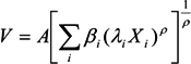
The CES function is applied in the product functions. The optimal combination of input factors is based on the following assumptions:
where,
Xi is the input factor
i;
Pi is the corresponding price;
V is the output;
βi is the share parameter of the factor
i;
A is the overall transformation parameter on all input factors;
λi is the transformation parameter on input factor
i;
ρ is a coefficient related to the substitution elasticity.
2.2. International Trade Module
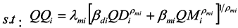
The substitutability between imported and domestically produced commodities is assumed to be imperfect in this study. Armington assumption, therefore, is applied to solve the problem. The domestically produced commodities and imported commodities are substitutable, they are not completely substitutable. The consumers can choose the best combination of imported and domestic commodities to minimize the costs. The function is shown as follows:
where
QDi refers to the domestic demand quantity of commodity
i,
PDi is the price;
QMi refers to the imported quantity of commodity
i,
PMi refers to the domestic price,
QQi refers to the total domestic demand quantity,
βdi and
βmi refer to the share parameters domestic and import commodity,
λmi is the overall transportation parameter between domestic supply and import demand of commodity
i,
ρmi is related substitution elasticity of import demand and domestic supply.
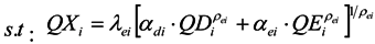
We adopt a constant elasticity transformation (CET) function to allocate total domestic output between exports and domestic sales. The function describes the optimal combinations between domestic sales and exports under a certain restriction of production technology. The function is shown as follows:
where
QDi refers to the domestic sale quantity of commodity
i,
PDi is the price;
QEi refers to the export quantity of commodity
i,
PEi refers to the domestic price,
QXi refers to the total domestic output,
αdi is the share parameter of domestic sales of commodity
i, and
αei is the share parameter of export of commodity
i,
λei is the overall transportation parameter between domestic sales and export of commodity
i,
ρei is related coefficient of the substitution elasticity.
2.3. Income and Expenditure
Household income is mainly from labor income, profit distribution from enterprises, and transfer payment from government and enterprises. Their income is used for consumption and saving. The consumption function complies with Stone-Geary utility function assumption. The specific functions are shown as below:
where,
YH is the households total disposable income (After-tax income minus household savings);
HDi is the households demand quantity of commodity
i;
θi is the minimum basic demand of commodity
i;
βi is the marginal propensity to consumption;
PQi is the demand price of commodity
i.
The enterprises’ income primarily comes from the capital revenue, and their expenditure mainly includes the transfer payment to the inhabitants and the income tax to the government. The left income is for enterprises’ savings. For the government, they get the income from indirect taxes, household and enterprises income tax, and tariff, while their expenditure includes transfer payment to the household and enterprises, government consumption, export rebate, and government savings.
2.4. Social Welfare Module
For the welfare function, we adopt Hicks Equivalent Variation. Based on commodity prices before the policy implementation, we calculate inhabitants’ utility through the demand changes by using the following formula:
where,
EV is the equivalent variation of inhabitants’ welfare, and
E(
Us,
PQb) is the utility after the policy implementation calculated by the payment function based on price before the policy implementation;
E(
Ub,
PQb) is the utility before the policy implementation;
![Sustainability 06 00487 i007]()
is the price of commodity
i before the policy implementation;
![Sustainability 06 00487 i008]()
and
![Sustainability 06 00487 i009]()
are the inhabitants’ consumption before and after the policy implementation, respectively.
EV is calculated by the formal formulas. Positive
EV means improvement in social welfare and the negative one means deterioration in social welfare after the implementation of the policy.
2.5. Carbon Tax Module
In this study, we assume that the carbon emissions mainly come from final consumption of coal, coke, crude oil, petroleum, natural gas, and gas. The carbon tax is calculated though multiplying the demand for various fossil energies by the rate of specific duty on each unit of carbon emissions, and the rate of specific duty on each unit of carbon emissions is endogenously decided under the given reduction target in this study. After converting the rate of specific duty into ad valorem tax rate, the demand price of the fossil energy will be (1+ ti) · PQi. ti is the ad valorem duty rate of fossil energy i, and PQi is the demand price of the fossil energy i. In doing so, the carbon tax will directly affect the input and demand cost of fossil energy, and, in turn, affect government revenue.
2.6. Model Closure and Market Clearing
The CGE model in this paper consider three principles of closure: government budget balance, foreign trade balance, and invest-saving balance. When considering the government budget balance, the government consumption is taken as exogenous variable, while government saving is endogenous. For the foreign trade balance, we assume exchange rate is designated endogenously while foreign savings is exogenous variable. The policy impacts on the exchange rate, and then the export and import are involved, even affects the whole economy. For the saving-investment balance, neo-classical closure principles are adopted. The investment is determined by the savings and all the savings in the economy system will be transferred to investment.
In this module, labor market, capital market, and commodity market are cleared by endogenous factor prices. The output of the model must be interpreted as a new equilibrium reached after the economy system has adjusted to the shock. The new equilibrium is the result of a mixture of different impacts, and the net effects of which cannot be derived analytically because the shock inevitably induce adjustments on several intertwined markets. Consequently, numerical simulations, therefore, are necessary in order to obtain the new equilibrium.
2.7. Dynamic Functions Model
The dynamic model mainly includes some functions related labor growth, technological progress level (Total Factor Productivity), and capital accumulation and allocation among sectors. In this paper, CET functions are applied to display the allocation of capital among sectors, and this allocation is determined by the sectoral capital revenue rate, the average rate of total capital, and the total supply of social capital. The functions of capital accumulation and allocation are shown as below.
where,
Ki,t is the capital demand of sector
i in
t period,
KSt is total supply of social capital in
t period,
TINVt is the total investment in
t period,
Ri,t is the capital revenue of sector
i in
t period,
ARt is the social capital average revenue in
t period,
depri is the capital depreciation rate of sector
i,
αi is the share parameter of capital requirement of sector
i,
ρ is the substitution parameter of capital among sectors.
3. Model Sectoral Structure
The CGE model in this paper is created by selecting 23 sectors, required for the carbon tax policy simulation. Most studies, which take the carbon tax policy of China as the research subject, usually integrate the mining and washing of coal sectors and coking sector into one sector, and integrate the petroleum extraction sector and refined oil sector into one sector. Factually, the energy consumption and carbon emissions are significantly different in the production process of those energy sectors. For example, the refined oil sector is unique in that it uses crude oil as a “feedstock” to produce refined oil products. The fuel combusted within petroleum refineries typically amounts to 6 to 10 percent of the total fuel input to the refinery, depending on the complexity and vintage of the technology (IPCC, 2006) [
28]. Similarly, coal is the important raw material in the coking process. Therefore, if those sectors are integrated into one sector, the feedstock input of crude oil or coal will be taken as the energy input, which may skew the results of policy simulation. According to the energy characteristics of China, this paper further disaggregate energy sectors into eight departments of coal, coke, crude oil, petroleum products, natural gas, gas, thermal power, and clean electricity, it is of great benefit to simulate the carbon tax’s impact on China’s economic development more accurately. The basic data are compiled from the 2007 Input–Output Table of China [
29].
In addition, the sector of extraction of petroleum and the sector of extraction natural gas are integrated into one sector, namely, the sector of extraction of petroleum and natural gas in the Input-Output Tables of China (the 1997 Input-Output Tables of China is an exception) [
30]. Disaggregating the sector of extraction of petroleum and natural gas into two sectors (that is, the sector of extraction of petroleum and the sector of extraction natural gas) is require for simulating the carbon tax policy since the input structure of production process and the allocation structure output of extraction of petroleum and extraction of natural gas are significantly different.
This paper takes the sum of the intermediate input rows and columns of Basic Flow Table of 2007 Input-Output Table [
29] as the control variables of row and column vectors, respectively. Then, we apply the RAS (Bi-proportional Scaling Method) method, which is an iterative method of bi-proportional adjustment to update the input-output table proposed by Stone in the 1960s, to compile the data of the sector of extraction petroleum and the sector of extraction natural gas. The data of inhabitants’ consumption, government consumption, investment, inventory, import, export, and value-added of Extraction of Petroleum and Natural Gas sectors, are obtained from the 2007 China Input-Output Table [
29] and the China Energy Statistical Yearbook [
31]. Thus, we adjust 42 and 135 sectors 2007 Input-Output Tables into 23 sectors according to the research need (see
Table 1).
5. Simulation Analyses of the Dynamic Benchmark Scenario
According to the parameter setting of benchmark scenario and the model simulation analyses,
Table 5 presents the variation characteristics of China’s GDP, the total energy consumption, energy consumption intensity, carbon emissions, and carbon emissions intensity under the benchmark scenario. It is shown that, from 2007 to 2030, China’s GDP will still grow rapidly. The GDP will increase from 26,604.381 billion Yuan in 2006 to 130,281.849 billion Yuan in 2030, but its growth rate will slow down. The economic growth rate mainly depends on the labor input, capital accumulation, and TFP. The main reason why the economic growth rate gradually decreases is that the capital accumulation is increasing compared with the labor input, leading to the gradual decrease of the marginal product of capital and the decrease of the GDP growth rate.
At the same time, the energy consumption and carbon emissions increase significantly during the simulation period. The energy consumption will increase by 3.04 times from 265.58 million tons standard coal in 2007 to 806.87 in 2030. The carbon emissions of fossil energy will rise by 3.01 times from 615.15 billion tons in 2007 to 1906.07 billion tons in 2030. However, the energy consumption intensity per unit of GDP, and carbon emissions intensity per unit of GDP gradually decline. The energy consumption intensity per unit of GDP will reduce form 0.9983 tons standard coal/104 Yuan in 2007 to 0.61933 tons standard coal/104 Yuan in 2030. The carbon emissions intensity per unit of GDP will reduce form 2.3122 tons/104 Yuan in 2007 to 1.4631 tons/104 Yuan in 2030. In a word, although the energy consumption intensity and carbon emissions intensity decrease significantly, the total energy consumption continues growing. Large amounts of carbon emissions, caused by energy consumption, will bring great environmental pressure.
Table 6 reveals China’s total primary energy consumption and its composition under the benchmark scenario. China’s primary energy consumption continues to increase with the increase of GDP. But the structure of primary energy consumption has been improved apparently. The proportion of coal in China’s total primary energy consumption will reduce from 69.50% in 2007 to 58.17% in 2030. The proportion of natural gas, hydropower, nuclear power, and wind power in China’s total primary energy consumption will go up significantly. The proportion of natural gas will increase from 3.50% in 2007 to 7.03% in 2030, and the proportion of hydropower, nuclear power, and wind power will increase from 7.30% in 2007 to 12.69% in 2030. The proportion of petroleum in China’s total primary energy consumption will rise slightly.
Under the benchmark scenario, the energy consumption intensity and carbon emission intensity decrease gradually. The optimization and upgrading of industrial structure in China is a major reason for gradual decline of energy consumption intensity.
Table 7 shows the development characteristics of China’s GDP and its composition under the benchmark scenario. From the simulation, we can see the proportion of China’s first industry in GDP will obviously reduce with a distinct increase for the proportion of China’s third industry from 38.88% in 2007 to 50.57% in 2030. For the proportion of the second industry with high-energy-consumption in GDP, it gradually drops from 50.35% in 2007 to 44.81% in 2030. Therefore, the energy consumption intensity per unit of GDP in China will gradually reduce due to the optimization of the industrial structure. Apart from this, the other reason is, during the simulation period, with the reduction of the output proportion of the second industry, the proportion of the output of capital goods sectors in the total output of the second industry will be unchanged or slightly higher because of the increased demand. As the energy industry being important sectors of the second industry, the proportion of its output in the total output will reduce gradually. Due to the relatively reduced supply, the cost of the energy input will, relatively, go up in the production process. Therefore, enterprises will increasingly improve the efficiency of energy inputs.
Table 6.
China’s total primary energy consumption and its composition (Benchmark scenario).
Table 6.
China’s total primary energy consumption and its composition (Benchmark scenario).
| Year | Total energy consumption | The proportion in total primary energies’ consumption |
|---|
| 104 tons standard coal | Coal | Petroleum | Natural gas | Hydro power, nuclear power, and wind power |
|---|
| 2007 | 265,583.00 | 69.50% | 19.70% | 3.50% | 7.30% |
| 2008 | 284,167.41 | 69.18% | 19.75% | 3.57% | 7.50% |
| 2009 | 304,393.76 | 68.82% | 19.81% | 3.65% | 7.71% |
| 2010 | 326,039.21 | 68.44% | 19.88% | 3.74% | 7.95% |
| 2011 | 347,990.11 | 68.01% | 19.99% | 3.84% | 8.16% |
| 2012 | 370,806.39 | 67.56% | 20.10% | 3.96% | 8.38% |
| 2013 | 394,372.07 | 67.09% | 20.22% | 4.08% | 8.61% |
| 2014 | 418,581.23 | 66.61% | 20.34% | 4.22% | 8.84% |
| 2015 | 443,339.81 | 66.11% | 20.45% | 4.37% | 9.07% |
| 2016 | 468,451.98 | 65.63% | 20.58% | 4.49% | 9.30% |
| 2017 | 493,936.92 | 65.14% | 20.70% | 4.62% | 9.54% |
| 2018 | 519,737.19 | 64.65% | 20.82% | 4.76% | 9.77% |
| 2019 | 545,808.60 | 64.16% | 20.93% | 4.91% | 10.01% |
| 2020 | 572,119.50 | 63.66% | 21.04% | 5.06% | 10.24% |
| 2021 | 596,432.42 | 63.11% | 21.17% | 5.23% | 10.50% |
| 2022 | 620,529.75 | 62.56% | 21.30% | 5.40% | 10.75% |
| 2023 | 644,412.30 | 62.01% | 21.42% | 5.58% | 11.00% |
| 2024 | 668,090.31 | 61.45% | 21.54% | 5.77% | 11.24% |
| 2025 | 691,582.07 | 60.90% | 21.65% | 5.96% | 11.49% |
| 2026 | 714,867.83 | 60.36% | 21.75% | 6.16% | 11.73% |
| 2027 | 738,002.17 | 59.81% | 21.85% | 6.37% | 11.98% |
| 2028 | 761,019.99 | 59.26% | 21.94% | 6.58% | 12.22% |
| 2029 | 783,961.01 | 58.72% | 22.03% | 6.80% | 12.45% |
| 2030 | 806,869.01 | 58.17% | 22.12% | 7.03% | 12.69% |
During the simulation period, the carbon emissions intensity decreases gradually. The main reasons are listed as follows: (1) the energy efficiency gradually increases; (2) the structure of primary energy consumption is gradually optimized with the decline of the proportion of coal in China’s total primary energy consumption and the increase of the proportion of clean power; and (3) the industrial structure is optimized and upgraded.
Generally speaking, under the benchmark scenario, China will keep a relatively high growth rate in economy, but the growth rate will slow down. The energy consumption structure and industrial structure will be optimized step by step. Through the energy consumption intensity per unit of GDP and carbon emissions intensity per unit of GDP decrease, total energy consumption will increase, and total CO2 emissions caused by a large amount of energy consumption will pose huge pressure on the environment in the future. The situation of energy-saving and emission-reduction will be grim.
Table 7.
Analysis of GDP and its composition (Benchmark scenario).
Table 7.
Analysis of GDP and its composition (Benchmark scenario).
| Year | GDP | The proportion of three industries |
|---|
| 109 Yuan | The primary industry | The secondary industry | The tertiary industry |
|---|
| 2007 | 266,043.81 | 10.77% | 50.35% | 38.88% |
| 2008 | 291,784.56 | 10.36% | 50.30% | 39.34% |
| 2009 | 319,534.13 | 9.95% | 50.23% | 39.82% |
| 2010 | 348,977.02 | 9.56% | 50.15% | 40.30% |
| 2011 | 378,873.57 | 9.11% | 50.08% | 40.81% |
| 2012 | 410,927.86 | 8.69% | 49.98% | 41.33% |
| 2013 | 445,106.89 | 8.30% | 49.87% | 41.83% |
| 2014 | 481,380.72 | 7.93% | 49.74% | 42.33% |
| 2015 | 519,724.50 | 7.59% | 49.59% | 42.82% |
| 2016 | 560,095.26 | 7.28% | 49.42% | 43.30% |
| 2017 | 602,500.84 | 6.99% | 49.24% | 43.77% |
| 2018 | 646,938.82 | 6.72% | 49.04% | 44.24% |
| 2019 | 693,416.10 | 6.48% | 48.83% | 44.69% |
| 2020 | 741,949.05 | 6.25% | 48.61% | 45.14% |
| 2021 | 790,685.52 | 6.05% | 48.26% | 45.69% |
| 2022 | 841,039.57 | 5.87% | 47.90% | 46.23% |
| 2023 | 893,030.58 | 5.71% | 47.52% | 46.77% |
| 2024 | 946,688.13 | 5.55% | 47.14% | 47.31% |
| 2025 | 1,002,051.62 | 5.41% | 46.74% | 47.85% |
| 2026 | 1,058,592.06 | 5.23% | 46.37% | 48.40% |
| 2027 | 1,116,874.21 | 5.07% | 45.99% | 48.94% |
| 2028 | 1,176,958.19 | 4.91% | 45.60% | 49.49% |
| 2029 | 1,238,913.42 | 4.76% | 45.21% | 50.03% |
| 2030 | 1,302,818.49 | 4.63% | 44.81% | 50.57% |
6. Simulation Analysis of Carbon Tax Policy
According to simulation analysis under the benchmark scenario, with China’s economic growth, energy consumption and carbon emissions will continue to increase and the situation of energy-saving and emission-reduction will be very serious in future. The carbon tax policy can be an effective tool to address climate changes, energy-saving, and emission-reduction. Therefore, we will analyze how the carbon tax and technical progress impact the energy consumption and carbon emissions in China. Three assumptions are adopted in the following scenarios.
Carbon tax scenario I: It is assumed that the carbon tax is implemented as of 2016. The annual carbon dioxide emissions will be reduced by 10% than under the benchmark scenario.
Carbon tax scenario II: It is assumed that the carbon tax is implemented as of 2016. The annual carbon dioxide emissions will be reduced by 10% than under the benchmark scenario. The enterprise income tax will be reduced accordingly, and the annual government revenue during the simulation period will be consistent with that in the benchmark scenario.
Table 8.
The analysis of GDP, energy consumption and carbon emission intensity (Scenario I).
Table 8.
The analysis of GDP, energy consumption and carbon emission intensity (Scenario I).
| Year | GDP | Percentage change of GDP | Total energy consumption | Percentage of change total energy consumption | Energy consumption intensity | Percentage change of energy consumption intensity | Carbon emissions intensity | Percentage change of carbon emissions intensity |
|---|
| 109 Yuan | 104 tons standard coal | ton standard coal/104 Yuan | tons/104 Yuan |
|---|
| 2016 | 559,532.02 | −0.1006% | 428,062.91 | −8.62% | 0.7650 | −8.53% | 1.7814 | −9.08% |
| 2017 | 601,896.78 | −0.1003% | 451,532.57 | −8.58% | 0.7502 | −8.49% | 1.7502 | −8.93% |
| 2018 | 646,293.14 | −0.0998% | 475,313.45 | −8.55% | 0.7354 | −8.46% | 1.7192 | −8.79% |
| 2019 | 692,726.81 | −0.0994% | 499,365.23 | −8.51% | 0.7209 | −8.41% | 1.6884 | −8.64% |
| 2020 | 741,212.83 | −0.0992% | 523,659.03 | −8.47% | 0.7065 | −8.38% | 1.6580 | −8.49% |
| 2021 | 789,908.34 | −0.0983% | 546,172.81 | −8.43% | 0.6914 | −8.33% | 1.6252 | −8.34% |
| 2022 | 840,217.98 | −0.0977% | 568,512.56 | −8.38% | 0.6766 | −8.29% | 1.5929 | −8.20% |
| 2023 | 892,159.56 | −0.0975% | 590,678.54 | −8.34% | 0.6621 | −8.25% | 1.5610 | −8.06% |
| 2024 | 945,761.04 | −0.0979% | 612,679.65 | −8.29% | 0.6478 | −8.20% | 1.5296 | −7.93% |
| 2025 | 1,001,060.16 | −0.0989% | 634,532.26 | −8.25% | 0.6339 | −8.16% | 1.4988 | −7.80% |
| 2026 | 1,057,523.87 | −0.1009% | 656,218.28 | −8.20% | 0.6205 | −8.11% | 1.4699 | −7.64% |
| 2027 | 1,115,717.24 | −0.1036% | 677,786.79 | −8.16% | 0.6075 | −8.07% | 1.4417 | −7.48% |
| 2028 | 1,175,698.62 | −0.1070% | 699,269.55 | −8.11% | 0.5948 | −8.02% | 1.4140 | −7.31% |
| 2029 | 1,237,535.64 | −0.1112% | 720,702.76 | −8.07% | 0.5824 | −7.97% | 1.3870 | −7.16% |
| 2030 | 1,301,305.14 | −0.1162% | 742,126.52 | −8.02% | 0.5703 | −7.91% | 1.3605 | −7.00% |
Carbon tax scenario III: It is assumed that the carbon tax policy is implemented as of 2016. The annual carbon dioxide emissions will be reduced by 10% than under the benchmark scenario. Technology of clean power is promoted, and total factor productivity will be one time higher than that under the benchmark scenario.
Thus, we analyze the influence of different policy scenarios on GDP, energy consumption, energy consumption structure, carbon emissions, and carbon emissions intensity.
Carbon tax scenario I: Due to the levy on carbon tax, GDP drops slightly from that in the benchmark scenario (see
Table 8). Specifically, due to the carbon tax, the input cost of fossil energy fuels increases, and the energy input of sectors reduces, leading to the reduction of the output and GDP to a certain extent. In another aspect, GDP will be equal to the final demand, because the increased prices of fossil energy fuels will cause the increase of the demand prices of the goods, resulting in the decrease of final demand. Due to the carbon tax, the cost of fossil energy fuels will rise. As a consequence, the total energy consumption decreases significantly by 8% of that under the benchmark scenario. For the total primary energy consumption and its composition (see
Table 9), coal carbon emission coefficient is big, thus, the carbon tax has an obvious influence on coal consumption, decreasing the proportion of coal in the total energy consumption significantly compared with under the benchmark scenario. However, the proportions of oil and natural gas increase slightly, and the proportion of clean power increases significantly, thus, the primary energy consumption structure is optimized to some extent. Accordingly, energy consumption intensity decreases about 8% than that under the benchmark scenario. Due to the decline of the total energy consumption and the coal proportion in primary energy structure, carbon emissions intensity reduces about 7%–9% above that in the benchmark scenario.
Table 9.
The total primary energy consumption and its composition (scenario I).
Table 9.
The total primary energy consumption and its composition (scenario I).
| Year | Total energy consumption | The proportion in total primary energies’ consumption |
|---|
| 104 tons standard coal | Coal | Petroleum | Natural gas | Hydro power, nuclear power, and wind power |
|---|
| 2016 | 428,062.91 | 62.52% | 22.34% | 4.76% | 10.38% |
| 2017 | 451,532.57 | 62.01% | 22.46% | 4.89% | 10.64% |
| 2018 | 475,313.45 | 61.51% | 22.57% | 5.03% | 10.89% |
| 2019 | 499,365.23 | 61.00% | 22.68% | 5.18% | 11.15% |
| 2020 | 523,659.03 | 60.50% | 22.78% | 5.33% | 11.40% |
| 2021 | 546,172.81 | 59.93% | 22.91% | 5.49% | 11.67% |
| 2022 | 568,512.56 | 59.37% | 23.03% | 5.66% | 11.94% |
| 2023 | 590,678.54 | 58.81% | 23.14% | 5.84% | 12.21% |
| 2024 | 612,679.65 | 58.25% | 23.25% | 6.02% | 12.48% |
| 2025 | 634,532.26 | 57.69% | 23.36% | 6.21% | 12.74% |
| 2026 | 656,218.28 | 57.14% | 23.45% | 6.41% | 13.00% |
| 2027 | 677,786.79 | 56.59% | 23.54% | 6.61% | 13.26% |
| 2028 | 699,269.55 | 56.05% | 23.62% | 6.82% | 13.52% |
| 2029 | 720,702.76 | 55.50% | 23.70% | 7.03% | 13.77% |
| 2030 | 742,126.52 | 54.95% | 23.78% | 7.25% | 14.02% |
Table 10.
The analysis of GDP, energy consumption and carbon emission intensity (Scenario II).
Table 10.
The analysis of GDP, energy consumption and carbon emission intensity (Scenario II).
| Year | GDP | Percentage change of GDP | Total energy consumption | Total energy consumption | Energy consumption intensity | Percentage change of energy consumption intensity | Carbon emissions intensity | Percentage change of carbon emissions intensity |
|---|
| 109 Yuan | 104 tons standard coal | ton standard coal/104 Yuan | tons/104 Yuan |
|---|
| 2016 | 576,714.99 | 2.97% | 430,573.33 | −8.09% | 0.7466 | −10.74% | 1.7309 | −11.66% |
| 2017 | 621,837.28 | 3.21% | 454,412.63 | −8.00% | 0.7308 | −10.86% | 1.6968 | −11.71% |
| 2018 | 668,995.26 | 3.41% | 478,559.94 | −7.92% | 0.7153 | −10.96% | 1.6637 | −11.73% |
| 2019 | 718,216.27 | 3.58% | 502,975.72 | −7.85% | 0.7003 | −11.03% | 1.6315 | −11.72% |
| 2020 | 769,148.52 | 3.67% | 527,602.03 | −7.78% | 0.6860 | −11.04% | 1.6008 | −11.65% |
| 2021 | 820,314.53 | 3.75% | 550,428.38 | −7.71% | 0.6710 | −11.04% | 1.5681 | −11.56% |
| 2022 | 872,682.85 | 3.76% | 573,046.91 | −7.65% | 0.6566 | −11.00% | 1.5368 | −11.43% |
| 2023 | 926,439.40 | 3.74% | 595,459.85 | −7.60% | 0.6427 | −10.93% | 1.5064 | −11.28% |
| 2024 | 981,437.00 | 3.67% | 617,670.27 | −7.55% | 0.6294 | −10.82% | 1.4771 | −11.09% |
| 2025 | 1,038,455.60 | 3.63% | 639,712.61 | −7.50% | 0.6160 | −10.75% | 1.4480 | −10.93% |
| 2026 | 1,097,026.70 | 3.63% | 661,586.46 | −7.45% | 0.6031 | −10.70% | 1.4202 | −10.76% |
| 2027 | 1,156,619.50 | 3.56% | 683,339.10 | −7.41% | 0.5908 | −10.59% | 1.3938 | −10.55% |
| 2028 | 1,217,649.90 | 3.46% | 704,981.02 | −7.36% | 0.5790 | −10.46% | 1.3684 | −10.31% |
| 2029 | 1,280,167.40 | 3.33% | 726,545.53 | −7.32% | 0.5675 | −10.31% | 1.3437 | −10.05% |
| 2030 | 1,344,204.80 | 3.18% | 748,071.28 | −7.29% | 0.5565 | −10.14% | 1.3199 | −9.78% |
Carbon tax scenario II: Compared with the benchmark scenario, GDP rises to a certain degree (see
Table 10). The reason is that although the carbon tax results in the improvement of production cost and the slight decrease of GDP, the carbon tax also leads to the reduction of enterprise income tax, which is then directly used for investment, directly boosting economy growth. Therefore, GDP even rises more than 3% under the benchmark scenario rather than decrease. At the same time, the total energy consumption decreases by 7%–8% than under the benchmark scenario. The energy consumption structures (see
Table 11) are obviously optimized, and the changes are consistent with those in scenario I. Compared with the benchmark scenario, the energy consumption intensity decreases nearly 10%–11%. Due to the growth of GDP, the energy consumption intensity drops more dramatically than in scenario I. The carbon emissions intensity also decreases significantly, compared with under the benchmark scenario. Generally speaking, reducing the enterprise income tax, when levying the carbon tax, will not only facilitate energy-saving and emission-reduction, but also bring certain growth of the GDP.
Table 11.
The total primary energy consumption and its composition (scenario II).
Table 11.
The total primary energy consumption and its composition (scenario II).
| Year | Total energy consumption | The proportion in total primary energies’ consumption |
|---|
| 104 tons standard coal | Coal | Petroleum | Natural gas | Hydro power, nuclear power, and wind power |
|---|
| 2016 | 430,573.33 | 61.23% | 22.91% | 4.90% | 10.97% |
| 2017 | 454,412.63 | 60.64% | 23.06% | 5.03% | 11.26% |
| 2018 | 478,559.94 | 60.07% | 23.21% | 5.18% | 11.54% |
| 2019 | 502,975.72 | 59.51% | 23.34% | 5.33% | 11.82% |
| 2020 | 527,602.03 | 58.98% | 23.46% | 5.48% | 12.08% |
| 2021 | 550,428.38 | 58.38% | 23.60% | 5.65% | 12.37% |
| 2022 | 573,046.91 | 57.82% | 23.72% | 5.82% | 12.64% |
| 2023 | 595,459.85 | 57.26% | 23.84% | 6.00% | 12.90% |
| 2024 | 617,670.27 | 56.73% | 23.94% | 6.18% | 13.15% |
| 2025 | 639,712.61 | 56.19% | 24.03% | 6.37% | 13.41% |
| 2026 | 661,586.46 | 55.65% | 24.12% | 6.56% | 13.68% |
| 2027 | 683,339.10 | 55.12% | 24.20% | 6.76% | 13.92% |
| 2028 | 704,981.02 | 54.61% | 24.27% | 6.96% | 14.16% |
| 2029 | 726,545.53 | 54.11% | 24.33% | 7.17% | 14.39% |
| 2030 | 748,071.28 | 53.61% | 24.38% | 7.39% | 14.62% |
Table 12.
The analysis of GDP, energy consumption and carbon emission intensity (Scenario III).
Table 12.
The analysis of GDP, energy consumption and carbon emission intensity (Scenario III).
| Year | GDP | Percentage change of GDP | Total energy consumption | Percentage change of total energy consumption | Energy consumption intensity | Percentage change of energy consumption intensity | Carbon emissions intensity | Percentage change of carbon emissions intensity |
|---|
| 109 Yuan | 104 tons standard coal | ton standard coal/104 Yuan | tons/104 Yuan |
|---|
| 2016 | 559,655.80 | −0.08% | 428,901.61 | −8.44% | 0.7664 | −8.37% | 1.7811 | −9.10% |
| 2017 | 602,166.88 | −0.06% | 453,356.92 | −8.22% | 0.7529 | −8.16% | 1.7495 | −8.97% |
| 2018 | 646,732.90 | −0.03% | 478,281.46 | −7.98% | 0.7395 | −7.95% | 1.7182 | −8.84% |
| 2019 | 693,360.41 | −0.01% | 503,645.91 | −7.72% | 0.7264 | −7.71% | 1.6871 | −8.71% |
| 2020 | 742,065.34 | 0.02% | 529,432.47 | −7.46% | 0.7135 | −7.48% | 1.6564 | −8.58% |
| 2021 | 791,003.22 | 0.04% | 553,621.21 | −7.18% | 0.6999 | −7.21% | 1.6234 | −8.45% |
| 2022 | 841,580.26 | 0.06% | 577,830.18 | −6.88% | 0.6866 | −6.94% | 1.5908 | −8.32% |
| 2023 | 893,815.02 | 0.09% | 602,068.79 | −6.57% | 0.6736 | −6.65% | 1.5587 | −8.20% |
| 2024 | 947,736.48 | 0.11% | 626,355.50 | −6.25% | 0.6609 | −6.35% | 1.5272 | −8.08% |
| 2025 | 1,003,383.66 | 0.13% | 650,716.71 | −5.91% | 0.6485 | −6.04% | 1.4962 | −7.96% |
| 2026 | 1,060,225.75 | 0.15% | 675,141.16 | −5.56% | 0.6368 | −5.70% | 1.4672 | −7.81% |
| 2027 | 1,118,828.93 | 0.18% | 699,691.21 | −5.19% | 0.6254 | −5.36% | 1.4388 | −7.66% |
| 2028 | 1,179,253.82 | 0.20% | 724,410.48 | −4.81% | 0.6143 | −5.00% | 1.4110 | −7.51% |
| 2029 | 1,241,570.72 | 0.21% | 749,348.09 | −4.42% | 0.6035 | −4.62% | 1.3838 | −7.37% |
| 2030 | 1,305,859.57 | 0.23% | 774,558.14 | −4.00% | 0.5931 | −4.22% | 1.3573 | −7.22% |
Carbon tax scenario III: When the carbon tax is levied and energy technology of clean power is improved, GDP grows slightly compared with that under the benchmark scenario, and the growth rate rises gradually (see
Table 12). We explain this as, although the costs of fossil energy fuels will rise, and enterprises’ energy inputs and outputs will fall due to carbon tax, the technology of clean power will be improved, and output of clean energy will increase, which is helpful for lowering the energy prices and promoting the use of clean power, therefore, GDP grows slightly compared with that under benchmark scenario, and the growth rate rises gradually.
Table 13 analyzes the total primary energy consumption and its composition, the proportion of coal in the primary energy consumption will drop to 52.58% by 2030, while the proportion of hydro power, nuclear power, and wind power will rise to 17.77% and the proportions of petroleum and natural gas are lower than those under the benchmark scenario. At the same time, compared with the benchmark scenario, the total energy consumption reduces slightly but in a decreased reduction rate, so does the trend of energy consumption intensity. In addition, due to the optimization of energy consumption structure, the carbon emissions intensity decreases more than 7%–9% each year compared with the benchmark scenario. Therefore, the improvement of clean power technology is significant to the optimization of energy consumption structure and carbon emission reductions. However, the cost reduction of the fossil energy fuels caused by the improvement of clean power technology partly improves the total energy demand.
Table 13.
The total primary energy consumption and its composition (scenario III).
Table 13.
The total primary energy consumption and its composition (scenario III).
| Year | Total energy consumption | The proportion in total primary energies’ consumption |
|---|
| 104 tons standard coal | Coal | Petroleum | Natural gas | Hydro power, nuclear power, and wind power |
|---|
| 2016 | 428,901.61 | 62.39% | 22.29% | 4.75% | 10.56% |
| 2017 | 453,356.92 | 61.76% | 22.35% | 4.87% | 11.01% |
| 2018 | 478,281.46 | 61.12% | 22.41% | 5.00% | 11.47% |
| 2019 | 503,645.91 | 60.47% | 22.46% | 5.13% | 11.94% |
| 2020 | 529,432.47 | 59.82% | 22.50% | 5.27% | 12.41% |
| 2021 | 553,621.21 | 59.11% | 22.56% | 5.42% | 12.91% |
| 2022 | 577,830.18 | 58.39% | 22.61% | 5.58% | 13.43% |
| 2023 | 602,068.79 | 57.67% | 22.65% | 5.74% | 13.94% |
| 2024 | 626,355.50 | 56.94% | 22.68% | 5.90% | 14.47% |
| 2025 | 650,716.71 | 56.22% | 22.71% | 6.07% | 15.00% |
| 2026 | 675,141.16 | 55.49% | 22.72% | 6.24% | 15.54% |
| 2027 | 699,691.21 | 54.77% | 22.72% | 6.42% | 16.09% |
| 2028 | 724,410.48 | 54.04% | 22.71% | 6.60% | 16.64% |
| 2029 | 749,348.09 | 53.31% | 22.70% | 6.79% | 17.20% |
| 2030 | 774,558.14 | 52.58% | 22.68% | 6.97% | 17.77% |


 is the price of commodity i before the policy implementation;
  and
and  are the inhabitants’ consumption before and after the policy implementation, respectively. EV is calculated by the formal formulas. Positive EV means improvement in social welfare and the negative one means deterioration in social welfare after the implementation of the policy.


