Quantitative Efficiency Evaluation Method for Transportation Networks

Abstract

An effective evaluation of transportation network efficiency/performance is essential to the establishment of sustainable development in any transportation system. Based on a redefinition of transportation network efficiency, a quantitative efficiency evaluation method for transportation network is proposed, which could reflect the effects of network structure, traffic demands, travel choice, and travel costs on network efficiency. Furthermore, the efficiency-oriented importance measure for network components is presented, which can be used to help engineers identify the critical nodes and links in the network. The numerical examples show that, compared with existing efficiency evaluation methods, the network efficiency value calculated by the method proposed in this paper can portray the real operation situation of the transportation network as well as the effects of main factors on network efficiency. We also find that the network efficiency and the importance values of the network components both are functions of demands and network structure in the transportation network.

1. Introduction

In recent years, with the development of the economy and urbanization, the number of motor vehicles in cities has increased significantly. However, due to the restrictions of land resources and environmental capacity, the imbalance between supply and demand in the urban transport system is becoming even more evident. This has further aggravated urban traffic congestion, which has resulted in reductions in vehicle travel speed, increased traffic delays, more accidents and deteriorating trends in terms of the environmental pollution. It is well-known that traffic congestion related to urban development has become an issue in most cities worldwide [1].

In attempts to solve this problem, two strategies were often adopted by transportation researchers and engineers. One strategy focuses on transportation supply and tries to promote rational development in the transportation system by increasing/upgrading transportation infrastructure supplies or plan-oriented management [2,3,4,5,6,7,8]. The other focuses on traffic demand by guiding and controlling traffic flows, such as traffic signal setting [9,10,11,12,13,14], parking pricing [15,16,17,18], or congestion pricing [19,20,21,22]. In these two strategies, decisions are mainly made based on the theory of traffic equilibrium assignment. Both strategies have their merits and disadvantages. Nevertheless, the essential factor—Transportation Network Efficiency (TNE)—which contributes to the coordination of transportation supply and traffic demand, has been neglected. In fact, TNE was not considered by the present solutions to traffic congestion, although all managements of transportation supply and demand were designed to increase the efficiency of transportation networks. The most important reason is that there is still no scientific method for the evaluation of TNE thus far, especially one that can be considered or used in mathematical models.

TNE comprehensively reflects the operation performance of a transportation network, which represents the common effect of traffic demands, travel costs and other factors on the network. A reasonable efficiency evaluation method for transportation networks can offer an objective analysis and measurement of the comprehensive operation status of a transportation network, which can in turn be used as guidance for the planning, reconstruction and maintenance of the network. In this way, problems resulting from the traditional single-factor methods for traffic congestion can be avoided.

With further study of transportation networks in recent years, the research refer to TNE is beginning and gradually becoming one of the main current research hotspots. In general, the existing efficiency evaluation methods for transportation networks can be classified into two categories: qualitative methods and quantitative methods.

The qualitative method for TNE is mainly based on the multi-index evaluation methods. Costa and Markellos [23] analyzed the productive efficiency of public transport services in cities, focusing on the competitive efficiency rather than the operation efficiency of the network. Levinson [24] evaluated the network efficiency with five indexes, which were mobility, utility, productivity, accessibility, and equity. Nait-Sidi-Moh et al. [25] evaluated the performance of the transit network, in which waiting time was the only indicator. This method actually only measured the coordination of the transit lines, but not the system efficiency. Therefore, the multi-index evaluation method mentioned above could reflect TNE to a certain extent can be concluded. However, as a consequence of its subjectivity, the objectivity and rationality of their results cannot be guaranteed. Researchers, such as Gudmundsson [26], Ming-Miin et al. [27] and Zhao et al. [28], have studied the ratio of input-to-output of the transportation network using the methods as Data Envelopment Analysis (DEA) or Stochastic Frontier Analysis (SFA). However, the network efficiency obtained from these methods still could not reflect the operation efficiency of the network, which only reflect the input-to-output on given indicators.

With regard to the quantitative methodologies, Roughgarden [29] used the travel costs to evaluate both the network efficiency and the loss of efficiency in different conditions. Wang et al. [30] and Xu et al. [31] measured the loss of the efficiency of selfish routing based on this method. Latora and Marchiori [32] proposed a method to measure network efficiency, in which the links may have associated weights or costs. This method was used in many studies related to complex network, such as Latora and Marchiori [33,34,35], and Crucitti et al. [36,37]. Chaug-Ing and Hsien-Hung [38] used it to measure the airline network either. However, the link congestion effects on the links were not considered in this method, which resulted in invalidation in measuring of TNE. Nagurney and Qiang [39,40], and Qiang and Nagurney [41] presented a quantitative efficiency evaluation method for transportation network, in which the parameters were only the number of origin-destination (OD) pairs, path flows and path travel costs, then the effect of network scale on the network efficiency was neglected.

Conclusively, the researches into TNE are still mainly based on the subjective multi-index evaluation method. The objective quantitative efficiency evaluation method cannot be used directly within a transportation network with regard to the congestion effect. Quantitative efficiency evaluation methods, which can be used in mathematical models for transportation networks, still remain to be improved.

This paper is organized as follows. In Section 2, a new definition of the TNE is presented. Then, we recall the well-known fixed demand network equilibrium model and propose various quantitative evaluation methods to compute the network efficiency value. Section 3 then presents a definition of the importance of network components in transportation networks. Furthermore, a network example is presented in Section 4, wherein the results from the new method are compared with those of Latora and Marchiori [32] and those of Jenelius et al. [42]. Section 5 summarizes the results in this paper and presents the conclusion.

2. Definition of TNE

TNE offers a comprehensive report of the performance of a transportation network, yet still does not have an explicit definition up to now. From the point of view of economics, efficiency always refers to the ratio of inputs (costs) to outputs (benefits) [43]. According to this definition, TNE is considered as “the degree of users satisfaction with the certain amount of transportation investments to traffic demand” [44]. However, on the one hand, indictors, which are used to describe “the degree of satisfaction”, are hard to be quantified. On the other hand, this definition cannot completely reflect the effects of network topology, travel choice behaviors, traffic demands and travel costs on TNE. Therefore, the above definition can hardly be applied to the quantitative evaluation of the operation status of a transportation network.

As mentioned earlier, some researchers regarded the total travel time/cost as the network efficiency and some valuable outcomes had been achieved [29,30,31,45]. However, the total travel time always goes up with the increase of network users in the transportation network. In other words, the network performance will always be inversely proportional to the amount of network users. Thus, it is widely believed that evaluation methods which only use travel time as the unique indicator could not faithfully reflect the actual operating performance of transportation network.

While the transportation network is a typical service-oriented network, the factors, such as network scale, traffic demands, and travel cost, should not be neglected when evaluating network efficiency/performance. Therefore, this paper tries to make a breakthrough with regard to discussing the limitation of former definitions of TNE, in which it can place more emphases on the transportation network users (drivers). Thus, we can redefine TNE as follows:

Definition 1. Transportation network efficiency

TNE refers to the quantity of traffic demands that can be met through a certain amount of investments in travel costs (network impedance) within the transportation network.

In the above TNE definition, traffic demands and travel costs are all easily quantified. Thus, the quantitative efficiency evaluation method is easier to be built using this definition compared to other definitions. Additionally, it is well-known that the improvement of TNE means that certain travel costs can service more traffic demands.

Rational TNE should reflect the effects of traffic demands, network structure/scale and travel choice on the performance of the transportation network. It is widely accepted that the traffic flows at equilibrium are the results of the interactions among these factors, which represent the usage of a network. In addition, the travel costs of the links, which are also important indicators, could help in the evaluation of the operation status of a transportation network. As a result, the link flows and the link travel costs at equilibrium in the transportation network can be considered as the main indicators in quantitative evaluation of the TNE.

From the analysis of TNE in this section, it is concluded that if we want to calculate the network efficiency, the link flows and the link travel costs at equilibrium need be calculated firstly. The traffic assignment problem is to find the traffic flows at equilibrium, to satisfy the user-equilibrium criterion when all the OD entries have been appropriately assigned. The transportation network equilibrium model need to be recalled, introduced by Sheffi [46], which is widely used in many research papersand in practices.

Consider a transportation network, $G=\left(N,A\right)$, in which N is the set of nodes and consists of n elements, A is the set of links with $n_A$ elements. W is the set of OD pairs of nodes with $n_W$ elements. The set of paths connecting OD pair $w\in W$ is denoted by $K_w$. The demand for OD pair $w$ is denoted by $q_w$. The flow and travel cost on link $a\in A$ are $x_a$ and $t_a\left(x_a\right)$, respectively. The flow on path $k\in K_w$ is denoted by $f_k^w$.

In this paper, we will consider link travel cost function $t_a\left(x_a\right)$ as Bureau of Public Road (BPR) functions, given by [46]:

$$t_a\left(x_a\right)=t_a^0\left(1+\alpha {\left(\frac{x_a}{c_a}\right)}^{\beta }\right)$$

(1)

Where $c_a$ is the capacity of link a, $t_a^0$ is the free-flow travel time or travel cost on link a. $\alpha$ and $\beta$ are the constant parameters and both take on positive values. Often $\alpha =0.15$ and $\beta =4$.

The indicator variable ${\delta }_{a,k}^w$ is set as:

$${\delta }_{a,k}^w=\{\begin{array}{l}1\text{\hspace{1em}if link a is on path k connecting OD pair w};\\ 0\text{\hspace{1em}otherwise}\end{array}$$

The link-flow pattern can be obtained by solving the flowing classical fixed demand traffic assignment model [46]:

$$MinZ\left(x\right)={\displaystyle \sum _{a\in A}{\displaystyle {\int }_0^{x_a}{t}_a\left(y\right)}{d}_y}$$

(2)

$$\text{s}.\text{t}. {\displaystyle \sum _{k\in K_w}{f}_k^w}=q_w,\forall w\in W$$

(3)

$$x_a={\displaystyle \sum _{w\in W}{\displaystyle \underset{k\in K_w}{ \sum }{f}_k^w{\delta }_{a,k}^w}},\forall a\in A$$

(4)

$$f_k^w\ge 0,\forall w\in W,\forall k\in K_w$$

(5)

In this model, the objective function Equation (2) is to minimize the total travel costs in the network. The function does not have any intuitive economic or behavioral interpretation, which should be viewed as a mathematical construct that is utilized to solve equilibrium problems. Equation (3) represents a set of flow conservations, which means that the sum of flows on paths connecting each OD pair $w$ must be equal to the demand between OD pair $w$. In other words, all OD demands have to be assigned to the network. The link flows are related to the path flows through the conservation of flow Equation (4), that is, the user cost on a path is equal to the sum of user costs on links that make up the path. Equation (5) is the nonnegative constraint on path flows, which ensure that the solution of the model will be physically meaningful.

There are many existing algorithms for the solutions of the above model Equations (2)–(5), such as the Frank-Wolfe (FW) and Gradient Projection (GP) methods. This paper does not focus on the solution method, thus, the classical GP method is chosen here to solve the model. The details of the GP method can be found in Qin et al. [47].

Thus far, quantitative evaluation methods for transportation networks have been rather rare, especially those that can be applied to TNE. Latora and Marchiori [32] proposed “global efficiency” to evaluate network performance in a weighted network. The method could be recalled as follows:

$$E=E\left(G\right)=\frac{1}{n\left(n-1\right)}{\displaystyle \sum _{i\ne j\in G}\frac{1}{d_{ij}}}$$

(6)

where E is the global efficiency; d_ij is the shortest path length (travel time) between the node i and node j at equilibrium, that is:

$$d_{ij}={\displaystyle \sum _{a\in k}{t}_a\left(x_a\right){\delta }_{a,k}^w},\forall k,w=\left(i,j\right)$$

In view of the congestion effects on the links in the transportation network, the lengths of the shortest paths between two nodes change with the traffic demands. In addition, the shortest path lengths are bound to increase with the growth of the demands in the transportation network. But according to Equation (6), efficiency E is a monotone decreasing function of demands. In this way, E will reach the maximum when the traffic flows on all links are 0, which is of course unreasonable. Therefore, measuring and analyzing the TNE with Equation (6) may lead to misleading results.

Here, a new quantitative efficiency evaluation method was proposed for the transportation networks, which is given in the following definition:

Definition 2. Efficiency evaluation method for transportation network

$$\epsilon =\epsilon \left(G,q\right)=\frac{1}{n_A}{\displaystyle \sum _{a\in A}\frac{{\overline{x}}_a}{{\overline{t}}_a}}$$

(7)

where $\text{ε}$ is the network efficiency; ${\overline{x}}_a$ and ${\overline{t}}_a$ are the flow and travel costs on link a at equilibrium respectively.

In an actual transportation network, the parameter ${\lambda }_a\ge 0$ for the link $a\in A$ can be added to Equation (6), so as to strengthen or weaken the impact of link a on $\epsilon$. Moreover, the generalized costs such as environmental costs can be added to the link travel costs ${\overline{x}}_a$.

The efficiency evaluation method presented in Equation (7) has a meaningful economic interpretation, since it evaluates the average efficiency/performance (link-based) of transportation networks from the perspective of the economic costs. This means that the efficiency can be considered as the average traffic to travel cost ratio with the equilibrium flow on link a being given by ${\overline{x}}_a$ and the equilibrium travel costs on link a denoted by ${\overline{t}}_a$. The effect of the network scale on the efficiency is measured by n_A. It is clear that the more traffic demands that can serve at a given cost, the higher the efficiency or performance of the transportation network performance is.

3. The Efficiency-Oriented Importance of the Transportation Network Component

To identify the critical components of a transportation network based on network efficiency, the definition of the “efficiency-oriented importance of the transportation network component” is given as follows:

Definition 3. Efficiency-oriented importance of transportation network component

The efficiency-oriented importance of a transportation network component is computed by relative drop of network efficiency value after it is completely blocked or failure in the network.

The network component here can be considered not only as a node or a link in the network, but also as several nodes or several links, and even a collection of some nodes and links (e.g., a path). In other words, a network component only needs to be a part of the transportation network.

The term “completely blocked or failure” in the definition can be explained as the removal of components from the transportation network. However, nodes and links in the network have different properties, so they need to be treated differently. For example, a link can be removed directly from a network. However, when a node is removed from a network, all the links connected to the node should be removed simultaneously. In addition, if removing a component causes some OD pairs to be disconnected in the network, it just need to be added a virtual path between the OD pairs and set the travel costs on the virtual path to infinity. It is believed that this definition is well-defined even in the case of disconnected networks.

According to the definition of the importance of network components, the importance value of a network component $g\in G$ could be computed as follows:

$$I_{\epsilon }\left(g\right)=\frac{\Delta \epsilon }{\epsilon }=\frac{\epsilon \left(G,d\right)-\epsilon \left(G-g,d\right)}{\epsilon \left(G,d\right)}$$

(8)

where $I_{\epsilon }\left(g\right)$ is the importance value of component g based on the efficiency $\text{ε}$; and G –g represents the resulting network after component g is removed from network G.

It is obvious that the upper bound of the importance value of a network component is 1. In addition, the greater the component importance value is, the more important it is to the performance of the transportation network.

Similarly, the importance value of the component $g\in G$ based on the global efficiency E could be measured as:

$$I_E\left(g\right)=\frac{\Delta E}{E}=\frac{E\left(G,d\right)-E\left(G-g,d\right)}{E\left(G,d\right)}$$

(9)

Jenelius et al. [42] also proposed several importance indicators for the links of road networks. In particular, they examined the use of these different link indicators depending on whether the removal of a link would cause the network to become disconnected or not. The definitions of these link importance indicators are briefly recalled in the following.

In the transportation network G = (N, A), for the link $a\in A$, the global importance I¹, the demand-weighted importance I², and the relative unsatisfied demand I³ are defined respectively, as follows(with the notations adapted to Section 2):

$$I^1\left(a\right)=\frac{1}{n_w}{\displaystyle \sum _{w\in W}\left({\lambda }_w\left(G-a\right)-{\lambda }_w\left(G\right)\right)}$$

(10)

$$I^2\left(a\right)=\frac{1}{{\displaystyle \sum _{w\in W}{q}_w}}{\displaystyle \sum _{w\in W}{\lambda }_w\left(G-a\right)-{\lambda }_w\left(G\right)}$$

(11)

$$I^3\left(a\right)=\frac{1}{{\displaystyle \sum _{w\in W}{q}_w}}{\displaystyle \sum _{w\in W}{u}_w\left(G-a\right)}$$

(12)

where ${\lambda }_w\left(G\right)$ is the original equilibrium travel cost of OD pair $w$; ${\lambda }_w\left(G-a\right)$ is the equilibrium travel cost of OD pair $w$ after link a is removed; and $u_w$ is the unsatisfied demands for OD pair $w$ after link a is removed.

If all the OD pairs remain connected after removing a link, then I¹ and I² would be applied to calculate the link importance values; otherwise I³ will be applied. Particularly, although these importance indicators consider the effects of the travel costs and the traffic flows, since they use different calculation formulas according to different situations, the importance values of the different components calculated from Equations (10)–(12) lack consistency, which results in difficulty in making a comprehensive comparison and judgment. These indictors would be compared with the approaches of Equations (8) and (9) in Section 5.

4. Numerical Examples

The network example is presented in this section. The transportation network efficiencies and the importance values of network components are calculated and ranked according to the different methods, respectively.

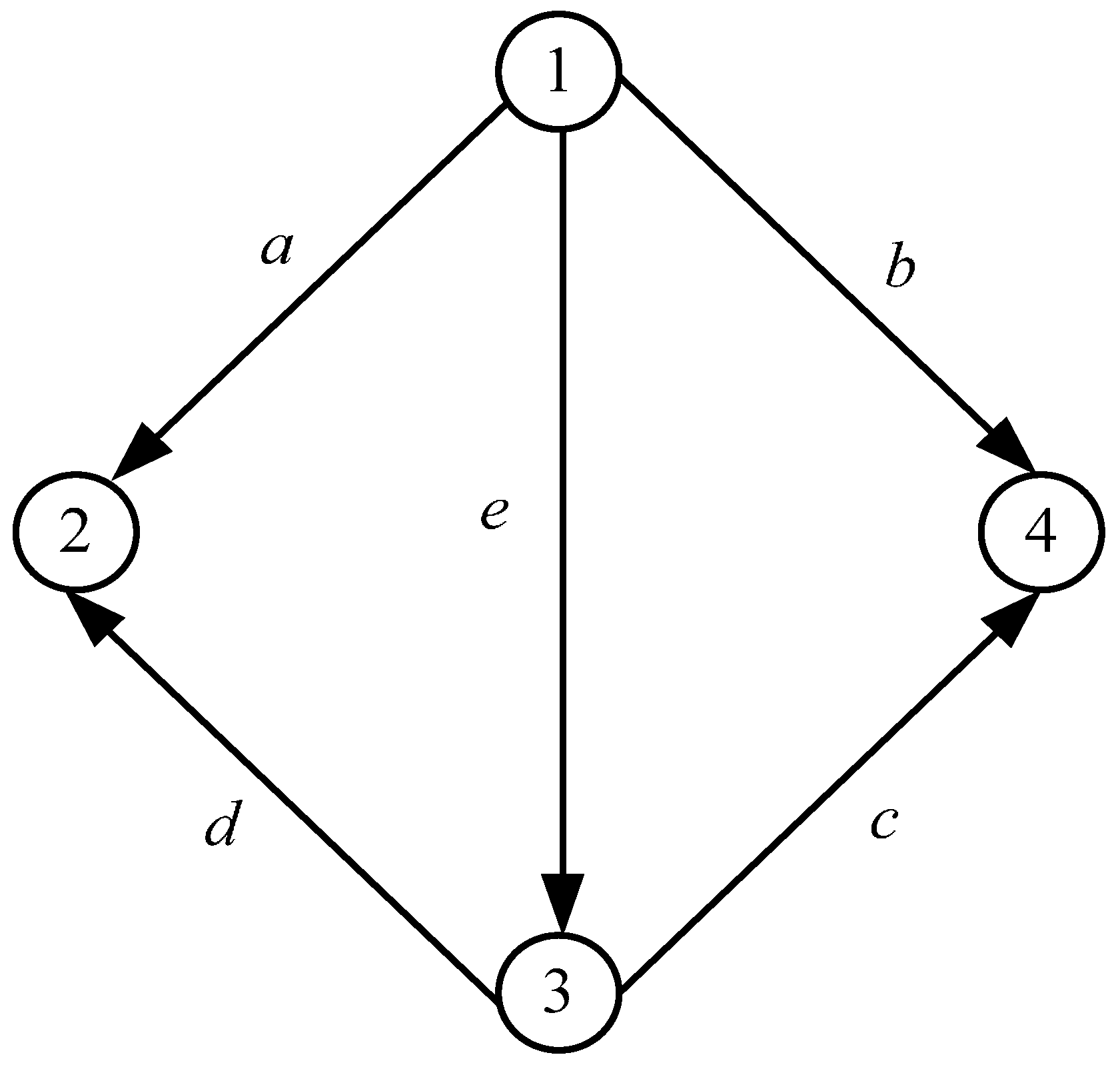
Consider the network in Figure 1, in which there are 5 OD pairs:(1,2), (1,4), (1,3), (3,2), (3,4). The traffic demands are given, respectively, by q₁₂ = 11, q₁₄ = 6, q₁₃ = 2, q₃₂ = 3, q₃₄ = 4.

Figure 1. The transportation network.

Figure 1. The transportation network.

Assume that the link travel cost BPR functions are given by:

$$t_a\left(x_a\right)=10\left(1+0.15{\left(\raisebox{1ex}{$x_a$}\!\left/ \!\raisebox{-1ex}{$4$}\right.\right)}^4\right)$$

(13)

$$t_b\left(x_b\right)=15\left(1+0.15{\left(\raisebox{1ex}{$x_b$}\!\left/ \!\raisebox{-1ex}{$6$}\right.\right)}^4\right)$$

(14)

$$t_c\left(x_c\right)=12\left(1+0.15{\left(\raisebox{1ex}{$x_c$}\!\left/ \!\raisebox{-1ex}{$3$}\right.\right)}^4\right)$$

(15)

$$t_d\left(x_d\right)=15\left(1+0.15{\left(\raisebox{1ex}{$x_d$}\!\left/ \!\raisebox{-1ex}{$10$}\right.\right)}^4\right)$$

(16)

$$t_e\left(x_e\right)=20\left(1+0.15{\left(\raisebox{1ex}{$x_e$}\!\left/ \!\raisebox{-1ex}{$8$}\right.\right)}^4\right)$$

(17)

As mentioned before, the GP method is utilized to solve the model Equations (2)–(5).

The computed link flows at equilibrium are as follows:

$$\overline{x}=\left\{{\overline{x}}_a,{\overline{x}}_b,{\overline{x}}_c,{\overline{x}}_d,{\overline{x}}_e\right\}=\left\{7.8107,5.7728,4.2272,6.1893,5.4165\right\}$$

(18)

Based on Equation (6), Equation (7) and $\overline{x}$, we could compute the efficiency $E=0.0195$, the efficiency ε = 0.2688, and the total travel cost is 120.5456.

4.1. Effects of Different Factors on TNE

Figure 2 shows that efficiency E changes with the traffic demand q₁₂ before and after removinglink a. Figure 3 shows the same changes of efficiency $\text{ε}$ with demand q₁₄ and link b.

Figure 2. Efficiency change with q₁₂ before and after removing link a.

Figure 2. Efficiency change with q₁₂ before and after removing link a.

Figure 3. Efficiency change with q₁₄ before and after removing link b.

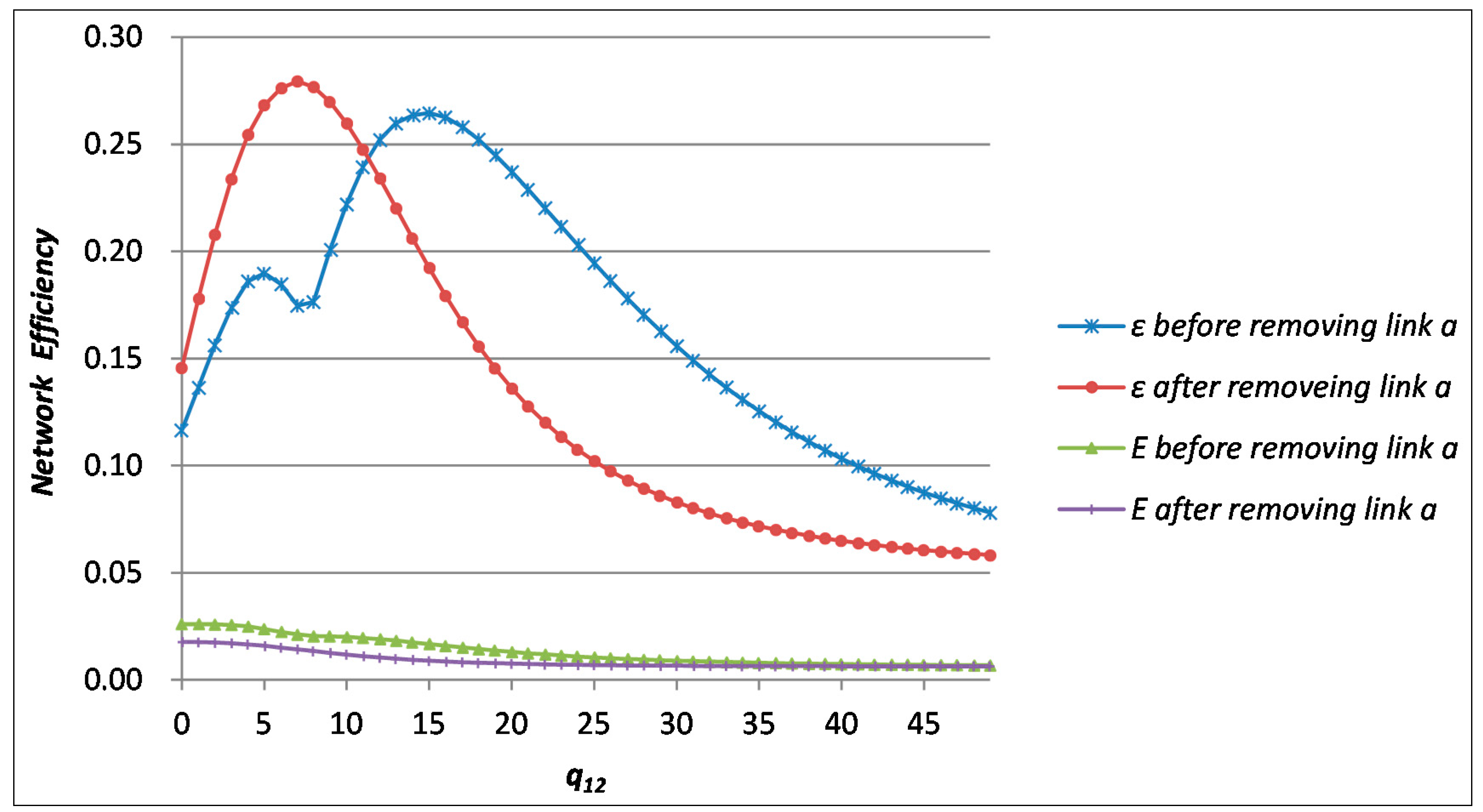
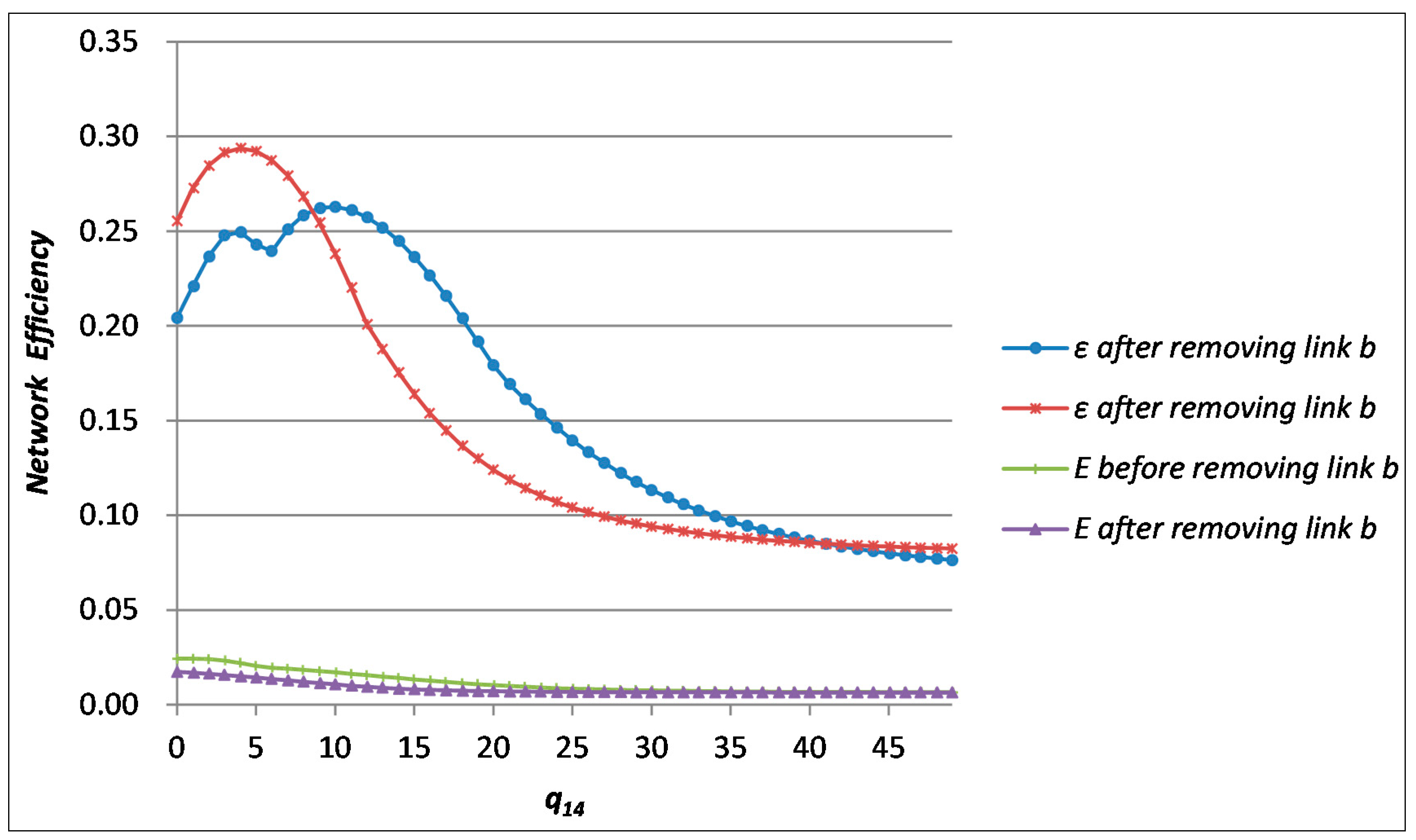
Figure 3. Efficiency change with q₁₄ before and after removing link b.

It is confirmed that efficiency E monotonously decreases, whether it occurs before or after the removal of links a and b. Moreover, the value of E before removing the links is always bigger than its value after removing them. Efficiency with the monotonous change can be considered as not describing how traffic demands and network structure affect network performance.

However, efficiency $\text{ε}$ is more reasonable in illustrating the effect that the demand and the network structure have on the network operation performance. From Figure 2, it is clear that $\text{ε}$ fluctuates with the change of demands, and there are two extreme points of $\text{ε}$ before removing link a, while there is only one after removing the link. The same results happen with link b in Figure 3. The reasons are that OD pairs (1,2) and (1,4) can be diverged with links a and b. In other words, there are two connected paths between OD pairs (1,2)/(1,4)before removing link a/b, but only one after removing the links. Obviously, this is consistent with the objective laws of transportation networks.

In the above two figures, we could see that sometimes after removing a link, the value of $\text{ε}$ is bigger than that before removing it. For example, when the rest of the demands remains the same, q₁₄ = 2, $\text{ε}$ are 0.237 and 0.285 before and after removing link b in Figure 3 respectively. Meanwhile, the total travel costs are 95.58 and 88.76, respectively. This indicates that the adding of link b will increase the total travel costs and reduce the network efficiency, which is known as the “Braess paradox” in transportation networks.

From Figure 3, we also could find that when $q_{14}\in [0,\mathrm{ 8}.435]$, $\text{ε}$ after removing link b will be higher than that before the removal, which proves that the “Braess paradox” phenomenon does happen. While q₁₄ > 8.435, $\text{ε}$ drops off after removing link b, which shows that the “Braess paradox” will not happen at this moment. The same result exists in the situations before and after removing link a.

The changes, that $\text{ε}$ increases after removing some links, happening within a specific range of traffic demands, are in conformity with the conclusions of Braess et al. [48].

On the basis of the analysis above, we could conclude the notable features of the TNE $\text{ε}$ are the following:

(1)

The TNE $\text{ε}$ is the function of the network structure/scale and traffic demands;

(2)

When the TNE $\text{ε}$ fluctuates with the demands in a given network structure, there is one or more extreme points. The number of extreme points is directly related to the number of paths connecting the changed OD pairs;

(3)

Fluctuations of the TNE $\text{ε}$ with the demands can be used to explain the “Braess paradox” in the transportation network.

4.2. Network Component Importance and Ranking from Different Methods

According to Equations (8) and (9), the node importance values and their rankings from different methods are reported in Table 1, respectively.

Table 1. The importance values and ranking of nodes according to different methods.

Node	$I_{\epsilon }\left(g\right)$	Ranking from $I_{\epsilon }\left(g\right)$	$I_E\left(g\right)$	Ranking from $I_E\left(g\right)$
1	0.4313	1	−0.2423	3
2	0.2885	2	−0.5849	4
3	0.0700	4	0.4327	1
4	0.1045	3	−0.2018	2

Table 1. The importance values and ranking of nodes according to different methods.

Node	$I_{\epsilon }\left(g\right)$	Ranking from $I_{\epsilon }\left(g\right)$	$I_E\left(g\right)$	Ranking from $I_E\left(g\right)$
1	0.4313	1	−0.2423	3
2	0.2885	2	−0.5849	4
3	0.0700	4	0.4327	1
4	0.1045	3	−0.2018	2

As the results showed in Table 1, node 1 is the most important node in the network according to $I_{\epsilon }\left(g\right)$, which is due to the fact that the two largest demands $q_{12}$ and $q_{14}$ are generated from it. In other words, node 1 has the largest flow among all the nodes in the network. Therefore, ranking the importance of node 1 in third place from $I_E\left(g\right)$ is obviously unreasonable.

In the network, the removal of links c, d or e will cause some OD pairs to be disconnected. Therefore, the importance indicators of these links must be measured with Equation (12). The rest of the links can be measured with Equation (10) and Equation (11). The importance values and rankings of links a, b, c, d and e calculated from Equations (8)–(12) are reported in Table 2, respectively.

Table 2. The importance values and ranking of links according to different methods.

Link	$I_{\epsilon }\left(g\right)$	Ranking from $I_{\epsilon }\left(g\right)$	$I_E\left(g\right)$	Ranking from $I_E\left(g\right)$	$I_1\left(k\right)$	Ranking from $I_1\left(k\right)$	$I_2\left(k\right)$	Ranking from $I_2\left(k\right)$	$I_3\left(k\right)$	Ranking from $I_3\left(k\right)$
a	0.0051	3	0.4045	1	23.418	1	6.6719	1
b	−0.1548	5	0.2456	4	10.309	2	2.7500	2
c	−0.1234	4	0.2420	5					0.0434	3
d	0.5004	1	0.3557	3					0.1304	1
e	0.4860	2	0.3717	2					0.0870	2

Table 2. The importance values and ranking of links according to different methods.

Link	$I_{\epsilon }\left(g\right)$	Ranking from $I_{\epsilon }\left(g\right)$	$I_E\left(g\right)$	Ranking from $I_E\left(g\right)$	$I_1\left(k\right)$	Ranking from $I_1\left(k\right)$	$I_2\left(k\right)$	Ranking from $I_2\left(k\right)$	$I_3\left(k\right)$	Ranking from $I_3\left(k\right)$
a	0.0051	3	0.4045	1	23.418	1	6.6719	1
b	−0.1548	5	0.2456	4	10.309	2	2.7500	2
c	−0.1234	4	0.2420	5					0.0434	3
d	0.5004	1	0.3557	3					0.1304	1
e	0.4860	2	0.3717	2					0.0870	2

From Table 2, we can see that the ranking from $I_{\epsilon }\left(g\right)$ is not consistent with the results of other methods. For example, link d should be the most important link from $I_{\epsilon }\left(g\right)$. However, according to $I_E\left(g\right)$, $I_1\left(k\right)$ and $I_2\left(k\right)$, link a has the highest importance value. In fact, the efficiency $\text{ε}$ and total travel costs after removing each link are reported in Table 3, from which we could know that removal of link d will cause the most negative influence on total travel costs, compared with the original travel cost 120.1734. Therefore, it is reasonable that the link d is the most important link in the network.

Table 3. Total travel costs and efficiency after removing links.

Removed Link	Total Travel Cost after Removing Link	ε after Removing Link	E after Removing Link
a	149.0294	0.2476	0.0110
b	117.3309	0.2874	0.0136
c	104.0035	0.2796	0.0152
d	165.7334	0.1248	0.0123
e	160.6061	0.1279	0.0126

Table 3. Total travel costs and efficiency after removing links.

Removed Link	Total Travel Cost after Removing Link	ε after Removing Link	E after Removing Link
a	149.0294	0.2476	0.0110
b	117.3309	0.2874	0.0136
c	104.0035	0.2796	0.0152
d	165.7334	0.1248	0.0123
e	160.6061	0.1279	0.0126

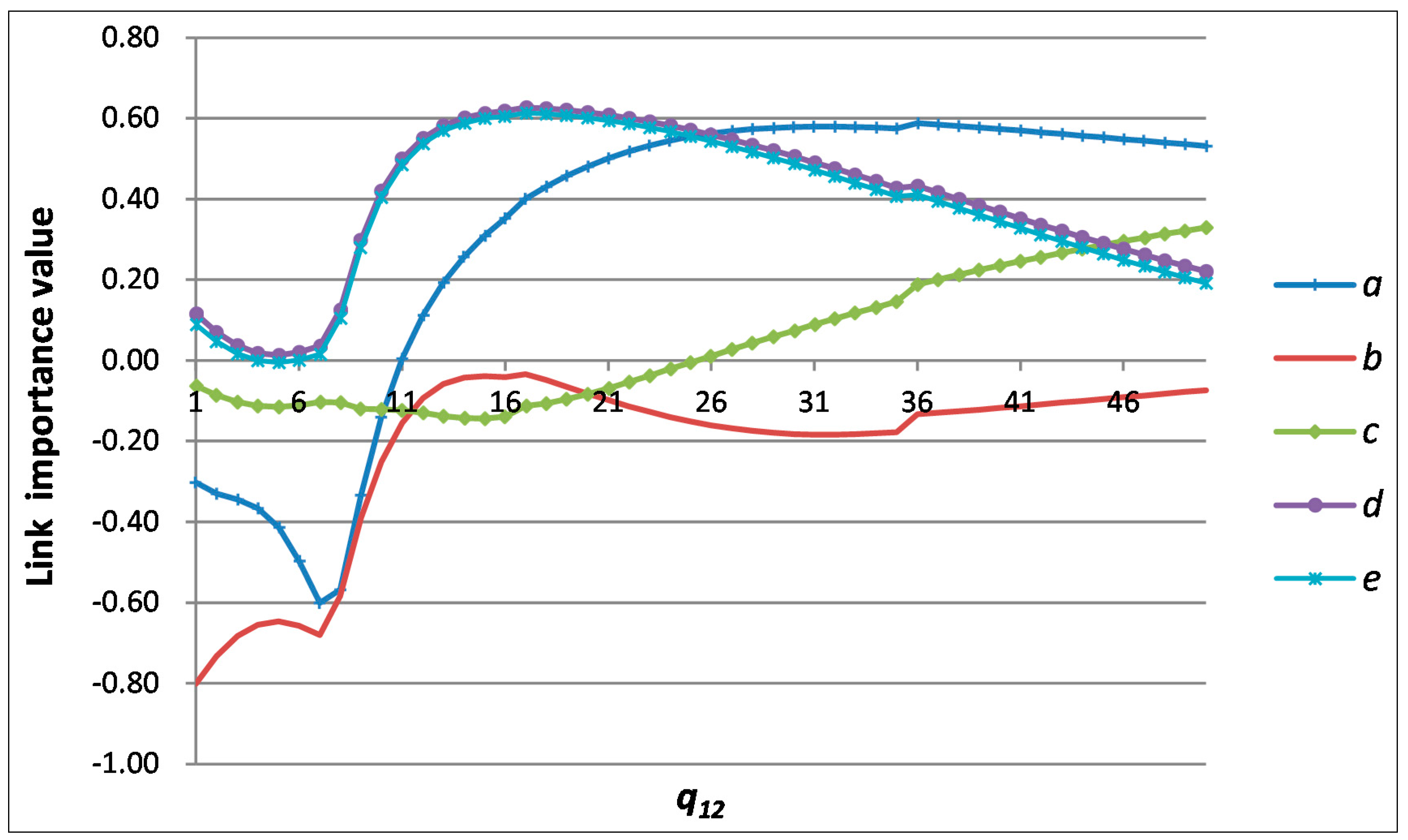
Figure 4 illustrates that the importance values of all links fluctuate with the demand $q_{12}$. And after $q_{12}$ reaches a specific value, the link a connecting node 1 with node 2 becomes the most important link in the network. This might be interpreted that the importance values $I_{\epsilon }\left(g\right)$, are the functions of the demands. In fact, we could find that same change in the importance value of nodes. So we could conclude that the network importance values $I_{\epsilon }\left(g\right)$ for nodes and links are all functions of the demands in the network.

Figure 4. Link importance $I_{\epsilon }\left(g\right)$ vs. $q_{12}$.

Figure 4. Link importance $I_{\epsilon }\left(g\right)$ vs. $q_{12}$.

Furthermore, the critical components of the transportation network can be identified based on the importance values of the network component. For example, the component importance values in descending order can be ranked at first. According to the ABC method, the top 20% of the components are the critical components, and the components ranked from 20% to 50% in the list are important components. Then the rest of the components are general components. The critical and important components have more important implications for network performance/vulnerability. Different maintenance or protection strategies should be implemented for different components. Obviously, the critical components must be more carefully monitored and serviced.

5. Conclusions

In this paper, we proposed a quantitative efficiency evaluation method for transportation networks, which can not only evaluate the operation efficiency/performance of a transportation network objectively, but also reflect how traffic demands, travel cost, travel choice behaviors and network structure (scale) affect transportation network operation. Based on the quantitative efficiency measure, the importance of network components, that is, nodes and links, were well-defined, even in a disconnected network, which could be used to identify the critical components in a transportation network.

Numerical examples showed that the TNE and importance values of network components, calculated by the methods proposed in this paper, all change with the network structure and demands, in other words, the efficiency value and the components’ importance values both are the functions of the structure and demands in the transportation network. In particular, the change of network efficiency can explain the “Braess paradox” in transportation network.

In addition, the paper has only analyzed the efficiency and the importance of network components in a fixed-demand transportation network. However, it should be noted that the conclusions would not be affected by the characteristics of traffic demands, since we only used traffic results at equilibrium, including flows and travel costs on links, in the quantitative efficiency evaluation of transportation networks.

References

- Berk, A.; Benjamin, H.; Tao, C. Spatio-temporal clustering for non-recurrent traffic congestion detection on urban road networks. Transp. Res. Part C 2014, 48, 47–65. [Google Scholar] [CrossRef]
- Boyce, D.E. Urban transportation network-equilibrium and design models: Recent achievements and future prospects. Environ. Plan. 1984, 16, 1445–1474. [Google Scholar] [CrossRef]
- Ben-Ayed, O.; Boyce, D.E.; Blair, C.E., III. A general bilevel linear programming formulation of the network design problem. Transp. Res. Part B 1988, 22, 311–318. [Google Scholar] [CrossRef]
- Cantarella, G.; Vitetta, A. The multi-criteria road network design problem in an urban area. Transportation 2006, 33, 567–588. [Google Scholar] [CrossRef]
- Chiou, S. Ahybrid approach for optimal design of signalized road network. Appl. Math. Model. 2008, 32, 195–207. [Google Scholar] [CrossRef]
- Dimitriou, L.; Stathopoulos, A.; Tsekeris, L. Reliable stochastic design of road network systems. Int. J. Ind. Syst. Eng. 2008, 3, 549–574. [Google Scholar]
- Grünig, M. Sustainable urban transport planning. Metrop. Sustain. 2012, 25, 607–624. [Google Scholar]
- Jia, Y.; Feng, S.; Zhao, Z.; Jin, Q. Combinatorial optimization of exclusive bus lanes and bus frequency based on multi-modal transportation network equilibrium. J. Transp. Eng. 2013, 138, 1422–1429. [Google Scholar]
- Cantarella, G.E.; Pavone, G.; Vitetta, A. Heuristics for urban road network design: Lane layout and signal settings. Eur. J. Oper. Res. 2006, 175, 1682–1695. [Google Scholar] [CrossRef]
- Cascetta, E.; Gallo, M.; Montella, B. Models and algorithms for the optimization of signal settings on urban networks with stochastic assignment. Ann. Oper. Res. 2006, 144, 301–328. [Google Scholar] [CrossRef]
- Di, W.; Yafeng, Y.; Siriphong, L.; Hai, Y. Design of more equitable congestion pricing and tradable credit schemes for multimodal transportation networks. Transp. Res. Part B 2012, 46, 1273–1287. [Google Scholar] [CrossRef]
- Lele, Z.; Timothy, M.G.; Jan, G. A comparative study of Macroscopic Fundamental Diagrams of arterial road networks governed by adaptive traffic signal systems. Transp. Res. Part B 2013, 49, 1–23. [Google Scholar]
- Qing, H.; Head, K.L.; Ding, J. Multi-modal traffic signal control with priority, signal actuation and coordination. Transp. Res. Part C 2014, 46, 65–82. [Google Scholar] [CrossRef]
- Ma, X.L.; Jin, J.C.; Lei, W. Multi-criteria analysis of optimal signal plans using microscopic traffic models. Transp. Res. Part D 2014, 32, 1–14. [Google Scholar] [CrossRef]
- Andrew, K.J.; Peter, C.J. Temporal variance of revealed preference on-street parking price elasticity. Transp. Policy 2009, 16, 193–199. [Google Scholar] [CrossRef]
- Fosgerau, M.; de Palma, A. The dynamics of urban traffic congestion and the price of parking. J. Pub. Econ. 2013, 105, 106–115. [Google Scholar] [CrossRef]
- Jos, O.; Derk, W.; Jasper, D. The real price of parking policy. J. Urban Econ. 2011, 70, 25–31. [Google Scholar] [CrossRef]
- Jos, O.; Giovanni, R. Time-varying parking prices. Econ. Transp. 2014, 3, 166–174. [Google Scholar] [CrossRef]
- Leape, J. The London congestion charge. J. Econ. Perspect. 2006, 20, 157–176. [Google Scholar] [CrossRef]
- Liu, S.Y.; Triantis, K.P.; Sarangi, S. A framework for evaluating the dynamic impacts of a congestion pricing policy for a transportation socioeconomic system. Transp. Res. Part A 2010, 44, 596–608. [Google Scholar]
- Lui, Z.Y.; Meng, Q.; Wang, S. Speed-based toll design for cordon-based congestion pricing scheme. Transp. Res. Part C 2013, 31, 83–98. [Google Scholar] [CrossRef]
- Jonas, E. The role of attitude structures, direct experience and reframing for the success of congestion pricing. Transp. Res. Part A 2014, 67, 81–95. [Google Scholar]
- Costa, A.; Markellos, R.N. Evaluating public transport efficiency with neural network models. Transp. Res. Part C 1997, 5, 301–312. [Google Scholar] [CrossRef]
- Levinson, D. Perspectives on efficiency in transportation. Int. J. Transp. Manag. 2003, 1, 45–155. [Google Scholar] [CrossRef]
- Nait-Sidi-Moh, A.; Manier, M.-A.; Moudni, A. Spectral analysis for performance evaluation in a bus network. Eur. J. Oper. Res. 2009, 193, 289–302. [Google Scholar] [CrossRef]
- Gudmundsson, S. Efficiency and performance measurement in the air transportation industry. Transp. Res. Part E 2004, 40, 439–442. [Google Scholar] [CrossRef]
- Yu, M.-M.; Lin, E.T.J. Efficiency and effectiveness in railway performance using a multi-activity network DEA model. Omega 2008, 36, 1005–1017. [Google Scholar] [CrossRef]
- Zhao, Y.; Triantisa, K.; Murray-Tuiteb, P.; Edarac, P. Performance measurement of a transportation network with a downtown space reservation system: A network-DEA approach. Transp. Res. Part E 2011, 6, 1140–1159. [Google Scholar] [CrossRef]
- Roughgarden, T. How bad is selfish routing. J. ACM 2002, 49, 236–259. [Google Scholar] [CrossRef]
- Wang, J.; Wei, D.; He, K.; Gong, H.; Wang, P. Encapsulating urban traffic rhythms into road networks. Sci. Rep. 2014, 4. Article 4141. [Google Scholar]
- Xu, Z.; Sun, L.; Wang, J.; Wang, P. The Loss of Efficiency Caused by Agents’ Uncoordinated Routing in Transport Networks. PLoS One 2014, 9, e111088. [Google Scholar] [CrossRef] [PubMed]
- Latora, V.; Marchiori, M. Efficient behavior of small-world networks. Phys. Rev. Lett. 2001, 87, 1–4. [Google Scholar] [CrossRef]
- Latora, V.; Marchiori, M. Economic small-world behavior in weighted networks. Eur. Phys. J. B 2002, 32, 249–263. [Google Scholar] [CrossRef]
- Latora, V.; Marchiori, M. Is the Boston subway a small-world network. Physica A 2002, 314, 109–113. [Google Scholar] [CrossRef]
- Latora, V.; Marchiori, M. How the science of complex networks can help developing strategies against terrorism. Chaos Soliton. Fract. 2004, 20, 69–75. [Google Scholar] [CrossRef]
- Crucitti, P.; Latora, V.; Marchiori, M. Efficiency of scale-free networks: Error and attack tolerance. Physica A 2003, 320, 622–642. [Google Scholar] [CrossRef]
- Crucitti, P.; Latora, V.; Marchiori, M. Error and attack tolerance of complex networks. Physica A 2004, 340, 388–394. [Google Scholar] [CrossRef]
- Hsu, C.-I.; Shih, H.-H. Small-world network theory in the study of network connectivity and efficiency of complementary international airline alliances. J. Air Transp. Manag. 2008, 14, 123–129. [Google Scholar] [CrossRef]
- Nagurney, A.; Qiang, Q. A network efficiency measure for congested networks. Europhys. Lett. 2007, 79, 1–5. [Google Scholar] [CrossRef]
- Nagurney, A.; Qiang, Q. A network efficiency measure with application to critical infrastructure networks. J. Glob. Optim. 2008, 40, 261–275. [Google Scholar] [CrossRef]
- Qiang, Q.; Nagurney, A. A unified network performance measure with importance identification and the ranking of network components. Optim. Lett. 2008, 2, 127–142. [Google Scholar] [CrossRef]
- Jenelius, E.; Petersen, T.; Mattsson, L. Importance and exposure in road network vulnerability analysis. Transp. Res. Part A 2006, 40, 537–560. [Google Scholar]
- Coelli, T.J.; Rao, D.S.P.; O’Donnell, C.J.; Battese, G.E. An Introduction to Efficiency and Productivity Analysis, 2nd ed.; Springer-Verlag New York Inc.: New York, NY, USA, 2005. [Google Scholar]
- Zhu, J. Research on Optimization Theory and Method of Urban Road Transportation System Based on Traffic Efficiency. Ph.D. Thesis, Southwest Jiaotong University, Chengdu, China, 2011. [Google Scholar]
- Yu, X.J.; Fang, C.H. Efficiency loss of mixed equilibrium associated with altruistic users and logit-based stochastic users in transportation network. PROMET—Traffic Transp. 2014, 26, 45–51. [Google Scholar]
- Sheffi, Y. Urban Transportation Networks: Equilibrium Analysis with Mathematical Programming Methods; Prentice-Hall Press: Englewood Cliffs, NJ, USA, 1985. [Google Scholar]
- Qin, J.; Ni, L.; Shi, F. Mixed Transportation Network Design under a Sustainable Development Perspective. Sci. World J. 2013, 2013, 549735. [Google Scholar]
- Braess, D.; Nagurney, A.; Wakolbinger, T. On a paradox of traffic planning. Transp. Sci. 2005, 39, 446–450. [Google Scholar] [CrossRef]
© 2014 by the authors; licensee MDPI, Basel, Switzerland. This article is an open access article distributed under the terms and conditions of the Creative Commons Attribution license (http://creativecommons.org/licenses/by/4.0/).
Share and Cite
MDPI and ACS Style
Qin, J.; He, Y.; Ni, L. Quantitative Efficiency Evaluation Method for Transportation Networks. Sustainability 2014, 6, 8364-8378. https://doi.org/10.3390/su6128364
AMA Style
Qin J, He Y, Ni L. Quantitative Efficiency Evaluation Method for Transportation Networks. Sustainability. 2014; 6(12):8364-8378. https://doi.org/10.3390/su6128364
Chicago/Turabian StyleQin, Jin, Yuxin He, and Linglin Ni. 2014. "Quantitative Efficiency Evaluation Method for Transportation Networks" Sustainability 6, no. 12: 8364-8378. https://doi.org/10.3390/su6128364