Sustainable and Resilient Supply Chain Network Design under Disruption Risks


Abstract
:
1. Introduction and Literature Review
2. Mathematical Model
2.1. Sets
| i, set of customer zones | i = {i|1, 2, …, I} |
| j, set of manufacturing zones | j = {j|1, 2, …, J} |
| k, set of warehouse zones | k = {k|1, 2, …, K} |
| l, set of suppliers | l = {l|1, 2, …, L} |
| t, set of different types of trucks | t = {t|1, 2, …, T} |
| p, set of periods | p = {t|1, 2, …, P} |
2.2. Parameters
| dip | Annual demand at customer zone i in period p |
| Mj | Cost of installing a manufacturing unit in zone j |
| Wk | Cost of installing a warehouse in zone k |
| UPClp | Purchase cost of material from supplier l ($/unit) in period p |
| ECFlp | Embodied carbon footprints of the material purchased from supplier l in period p |
| TCSMljtp | Transportation cost from supplier l to manufacturing zone j using truck t ($/unit) in period p |
| TCMWjktp | Transportation cost from manufacturing zone j to warehouse zone k using truck t ($/unit) in period p |
| TCWCkitp | Transportation cost from warehouse zone k to customer zone i using truck t ($/unit) in period p |
| HCSMljp | Handling cost from supplier l to manufacturing unit in zone j ($/unit) in period p |
| HCMWjkp | Handling cost from manufacturing zone j to warehouse in zone k ($/unit) in period p |
| HCWCkip | Handling cost from warehouse in zone k to customer zone i ($/unit) in period p |
| CESMljtp | Carbon emission by truck t from supplier l to manufacturing zone j (kg/unit) in period p |
| CEMWjktp | Carbon emission by truck t from manufacturing zone j to warehouse zone k (kg/unit) in period p |
| CEWCkitp | Carbon emission by truck t from warehouse zone k to customer zone i (kg/unit) in period p |
| MCjp | Manufacturing cost at zone j ($/unit) in period p |
| CEj | Carbon emission by manufacturing unit in zone j (kg/unit) |
| CSlp | Capacity of supplier l in period p |
| CMjp | Capacity of manufacturing unit in zone j in period p |
| CTtp | Capacity of truck t in period p |
| CWkp | Capacity of inventory in warehouse k in period p |
| PMp | Profit margin on each unit in period p |
| sdlp | Supplier’s disruption probability in period p |
| mdjp | Manufacturing zone’s disruption probability in period p |
| wdkp | Warehouse zone’s disruption probability in period p |
2.3. Decision Variables
 | If a warehouse in zone k is open 1, otherwise 0 |
 | If a manufacturing unit in zone j is open 1, otherwise 0 |
| TQSMljtp | Transportation quantity from supplier l to manufacturing zone j using truck t in period p |
| TQMWjktp | Transportation quantity from manufacturing zone j to warehouse zone k using truck t in period p |
| TQWCkitp | Transportation quantity from warehouse zone k to customer zone i using truck t in period p |
2.4. Deviational Variables
 , ,  | Under and over achievement from total supply chain cost goal |
 , ,  | Under and over achievement from carbon emission goal |
 , ,  | Under and over achievement from embodied carbon footprint goal |
 , ,  | Under and over achievement from disruption cost goal as a measure of resilience |
2.5. Model
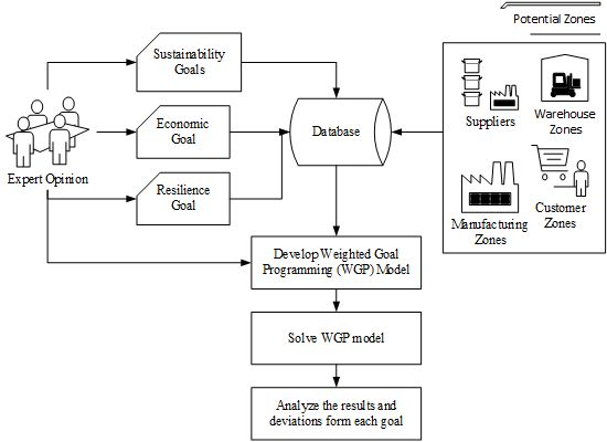
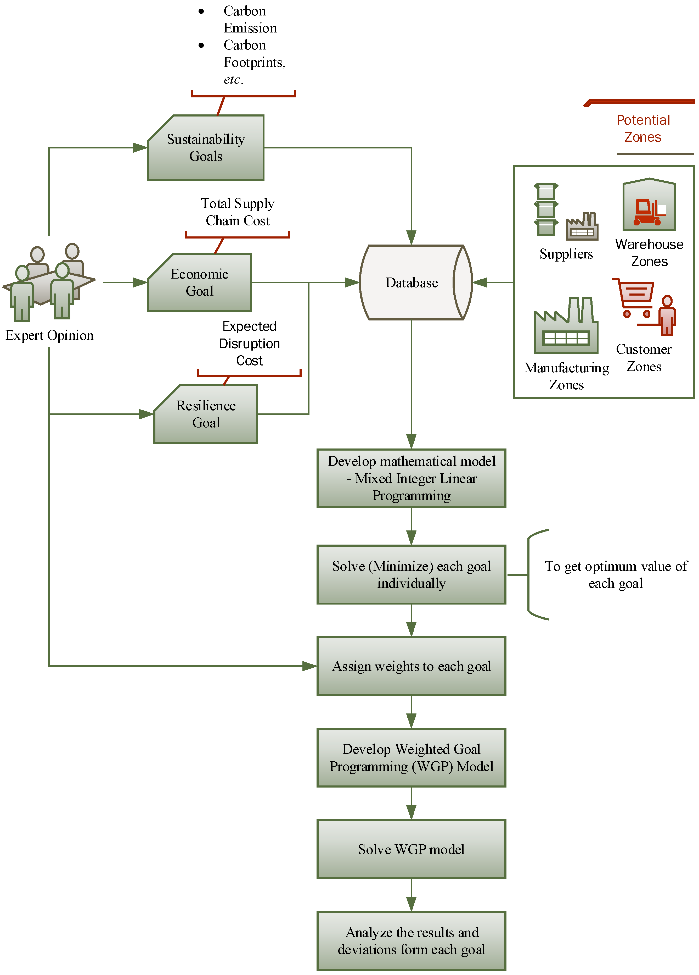
 , , and represent the deviational variables of cost, carbon emission, embodied carbon footprints and resilient supply chain goals, respectively, and β1, β2, β3 and β4 are the corresponding weights of the above objective deviations. It is important to recognize in Equation (1) that deviations of goals are measured in different units, i.e., $ and kg; therefore, we cannot sum them directly due to the phenomenon of incommensurability. Percentage normalization is used in the proposed model to standardize the unit in the objective function. Percentage normalization is carried out by dividing the deviations with their corresponding target levels. Thus, all deviations are measured in the same units, as shown in Equation (2).


3. Case Example

| Region No. | Region Name | No. of Manmade Disasters | No. of Natural Disasters | Probability |
|---|---|---|---|---|
| 1 | Faisalabad | 00 | 01 | 0.003 |
| 2 | Hyderabad | 03 | 00 | 0.010 |
| 3 | Karachi | 86 | 02 | 0.280 |
| 4 | Lahore | 05 | 04 | 0.029 |
| 5 | Peshawar | 53 | 01 | 0.172 |
| 6 | Quetta | 54 | 01 | 0.175 |
| 7 | Rawalpindi | 04 | 00 | 0.013 |
| Period | ||||
|---|---|---|---|---|
| 1 | 2 | 3 | ||
| Supplier | 1 | 4.119 | 4.609 | 4.392 |
| 2 | 4.016 | 4.588 | 5.654 | |
| 3 | 4.911 | 5.016 | 5.516 | |
| Period | ||||
|---|---|---|---|---|
| 1 | 2 | 3 | ||
| Supplier | 1 | 2.4 | 2.7 | 2.8 |
| 2 | 1.9 | 2.0 | 2.2 | |
| 3 | 1.5 | 1.8 | 2.1 | |
| Period | Supplier 1 | Supplier 2 | Supplier 3 | |||||||
|---|---|---|---|---|---|---|---|---|---|---|
| 1 | 2 | 3 | 1 | 2 | 3 | 1 | 2 | 3 | ||
| Manufacturing Zones | 1 | 0.010 | 0.010 | 0.020 | 0.015 | 0.020 | 0.010 | 0.015 | 0.013 | 0.011 |
| 2 | 0.020 | 0.011 | 0.014 | 0.010 | 0.012 | 0.014 | 0.011 | 0.013 | 0.012 | |
| 3 | 0.009 | 0.008 | 0.010 | 0.008 | 0.009 | 0.020 | 0.011 | 0.012 | 0.013 | |
| Period | Manufacturing Zone 1 | Manufacturing Zone 2 | Manufacturing Zone 3 | |||||||
|---|---|---|---|---|---|---|---|---|---|---|
| 1 | 2 | 3 | 1 | 2 | 3 | 1 | 2 | 3 | ||
| Warehouse Zones | 1 | 0.010 | 0.020 | 0.009 | 0.015 | 0.019 | 0.020 | 0.011 | 0.014 | 0.013 |
| 2 | 0.015 | 0.011 | 0.014 | 0.013 | 0.014 | 0.016 | 0.012 | 0.019 | 0.013 | |
| 3 | 0.020 | 0.015 | 0.020 | 0.008 | 0.012 | 0.020 | 0.013 | 0.020 | 0.015 | |
| 4 | 0.015 | 0.011 | 0.014 | 0.013 | 0.014 | 0.016 | 0.012 | 0.019 | 0.013 | |
| Period | Warehouse Zone 1 | Warehouse Zone 2 | Warehouse Zone 3 | Warehouse Zone 4 | |||||||||
|---|---|---|---|---|---|---|---|---|---|---|---|---|---|
| 1 | 2 | 3 | 1 | 2 | 3 | 1 | 2 | 3 | 1 | 2 | 3 | ||
| Customer Zones | 1 | 0.010 | 0.015 | 0.020 | 0.020 | 0.016 | 0.020 | 0.014 | 0.012 | 0.011 | 0.012 | 0.011 | 0.011 |
| 2 | 0.020 | 0.011 | 0.015 | 0.015 | 0.012 | 0.013 | 0.012 | 0.019 | 0.015 | 0.015 | 0.016 | 0.013 | |
| 3 | 0.008 | 0.009 | 0.011 | 0.011 | 0.015 | 0.020 | 0.015 | 0.016 | 0.013 | 0.012 | 0.019 | 0.013 | |
| 4 | 0.010 | 0.011 | 0.011 | 0.02 | 0.015 | 0.02 | 0.025 | 0.028 | 0.025 | 0.028 | 0.029 | 0.030 | |
| 5 | 0.020 | 0.011 | 0.015 | 0.015 | 0.012 | 0.013 | 0.012 | 0.019 | 0.015 | 0.015 | 0.016 | 0.013 | |
 ) from suppliers to manufacturing zones by different trucks at different periods.
| Period | Truck Type 1 | Truck Type 2 | Truck Type 3 | |||||||||
|---|---|---|---|---|---|---|---|---|---|---|---|---|
| 1 | 2 | 3 | 1 | 2 | 3 | 1 | 2 | 3 | ||||
| Supplier | 1 | Manufacturing Zone | 1 | 6.57 | 6.57 | 6.57 | 2.55 | 2.55 | 2.55 | 1.91 | 1.91 | 1.91 |
| 2 | 47.4 | 47.4 | 47.4 | 18.4 | 18.4 | 18.4 | 13.8 | 13.8 | 13.8 | |||
| 3 | 340.0 | 340.0 | 340.0 | 132.2 | 132.2 | 132.2 | 99.1 | 99.1 | 99.1 | |||
| 2 | Manufacturing Zone | 1 | 47.4 | 47.4 | 47.4 | 18.4 | 18.4 | 18.4 | 13.8 | 13.8 | 13.8 | |
| 2 | 2.85 | 2.85 | 2.85 | 1.11 | 1.11 | 1.11 | 8.33 | 8.33 | 8.33 | |||
| 3 | 300.0 | 300.0 | 300.0 | 116.6 | 116.6 | 116.6 | 87.5 | 87.5 | 87.5 | |||
| 3 | Manufacturing Zone | 1 | 340.0 | 340.0 | 340.0 | 132.2 | 132.2 | 132.2 | 99.1 | 99.1 | 99.1 | |
| 2 | 300.0 | 300.0 | 300.0 | 116.6 | 116.6 | 116.6 | 87.5 | 87.5 | 87.5 | |||
| 3 | 2.85 | 2.85 | 2.85 | 1.11 | 1.11 | 1.11 | 8.33 | 8.33 | 8.33 | |||
) from manufacturing zones to warehouse zones by different trucks at different periods.
| Period | Truck Type 1 | Truck Type 2 | Truck Type 3 | |||||||||
|---|---|---|---|---|---|---|---|---|---|---|---|---|
| 1 | 2 | 3 | 1 | 2 | 3 | 1 | 2 | 3 | ||||
| Manufacturing Zone | 1 | Warehouse Zone | 1 | 6.57 | 6.57 | 6.57 | 2.56 | 2.56 | 2.56 | 1.92 | 1.92 | 1.92 |
| 2 | 349.0 | 349.0 | 349.0 | 136.0 | 136.0 | 136.0 | 102.0 | 102.0 | 102.0 | |||
| 3 | 206.0 | 206.0 | 206.0 | 80.1 | 80.1 | 80.1 | 60.1 | 60.1 | 60.1 | |||
| 4 | 387.0 | 387.0 | 387.0 | 150.0 | 150.0 | 150.0 | 113.0 | 113.0 | 113.0 | |||
| 2 | Warehouse Zone | 1 | 47.4 | 47.4 | 47.4 | 18.4 | 18.4 | 18.4 | 13.8 | 13.8 | 13.8 | |
| 2 | 311.0 | 311.0 | 311.0 | 121.0 | 121.0 | 121.0 | 90.6 | 90.6 | 90.6 | |||
| 3 | 205.0 | 205.0 | 205.0 | 79.6 | 79.6 | 79.6 | 59.7 | 59.7 | 59.7 | |||
| 4 | 344.0 | 344.0 | 344.0 | 134.0 | 134.0 | 134.0 | 100.0 | 100.0 | 100.0 | |||
| 3 | Warehouse Zone | 1 | 340.0 | 340.0 | 340.0 | 132.0 | 132.0 | 132.0 | 92.2 | 92.2 | 92.2 | |
| 2 | 43.4 | 43.4 | 43.4 | 16.9 | 16.9 | 16.9 | 12.7 | 12.7 | 12.7 | |||
| 3 | 234.0 | 234.0 | 234.0 | 91.1 | 91.1 | 91.1 | 68.3 | 68.3 | 68.3 | |||
| 4 | 147.0 | 147.0 | 147.0 | 57.3 | 57.3 | 57.3 | 43.0 | 43.0 | 43.0 | |||
) from warehouse zones to customer zones by different trucks at different periods.
| Period | Truck Type 1 | Truck Type 2 | Truck Type 3 | |||||||||
|---|---|---|---|---|---|---|---|---|---|---|---|---|
| 1 | 2 | 3 | 1 | 2 | 3 | 1 | 2 | 3 | ||||
| Warehouse Zone | 1 | Customer Zone | 1 | 6.57 | 6.57 | 6.57 | 2.56 | 2.56 | 2.56 | 1.92 | 1.92 | 1.92 |
| 2 | 350.0 | 350.0 | 350.0 | 136.0 | 136.0 | 136.0 | 102.0 | 102.0 | 102.0 | |||
| 3 | 206.0 | 206.0 | 206.0 | 80.1 | 80.1 | 80.1 | 60.1 | 60.1 | 60.1 | |||
| 4 | 411.0 | 411.0 | 411.0 | 160.0 | 160.0 | 160.0 | 120.0 | 120.0 | 120.0 | |||
| 5 | 387.0 | 387.0 | 387.0 | 150.0 | 150.0 | 150.0 | 113.0 | 113.0 | 113.0 | |||
| 2 | Customer Zone | 1 | 350.0 | 350.0 | 350.0 | 136.0 | 136.0 | 136.0 | 102.0 | 102.0 | 102.0 | |
| 2 | 2.86 | 2.86 | 2.86 | 1.11 | 1.11 | 1.11 | 0.83 | 0.83 | 0.83 | |||
| 3 | 266.0 | 266.0 | 266.0 | 103.0 | 103.0 | 103.0 | 77.5 | 77.5 | 77.5 | |||
| 4 | 105.0 | 105.0 | 105.0 | 40.7 | 40.7 | 40.7 | 30.5 | 30.5 | 30.5 | |||
| 5 | 135.0 | 135.0 | 135.0 | 52.3 | 52.3 | 52.3 | 39.3 | 39.3 | 39.3 | |||
| 3 | Customer Zone | 1 | 206.0 | 206.0 | 206.0 | 80.1 | 80.1 | 80.1 | 60.1 | 60.1 | 60.1 | |
| 2 | 266.0 | 266.0 | 266.0 | 103.0 | 103.0 | 103.0 | 77.5 | 77.5 | 77.5 | |||
| 3 | 2.86 | 2.86 | 2.86 | 1.11 | 1.11 | 1.11 | 8.33 | 8.33 | 8.33 | |||
| 4 | 257.0 | 257.0 | 257.0 | 100.0 | 100.0 | 100.0 | 75.0 | 75.0 | 75.0 | |||
| 5 | 241.0 | 241.0 | 241.0 | 93.8 | 93.8 | 93.8 | 70.3 | 70.3 | 70.3 | |||
| 4 | Customer Zone | 1 | 387.0 | 387.0 | 387.0 | 150.0 | 150.0 | 150.0 | 113.0 | 113.0 | 113.0 | |
| 2 | 135.0 | 135.0 | 135.0 | 52.3 | 52.3 | 52.3 | 39.3 | 39.3 | 39.3 | |||
| 3 | 241.0 | 241.0 | 241.0 | 93.8 | 93.8 | 93.8 | 70.3 | 70.3 | 70.3 | |||
| 4 | 48.3 | 48.3 | 48.3 | 18.8 | 18.8 | 18.8 | 14.1 | 14.1 | 14.1 | |||
| 5 | 2.86 | 2.86 | 2.86 | 1.11 | 1.11 | 1.11 | 8.33 | 8.33 | 8.33 | |||
 ) for raw material transportation from suppliers to manufacturing zones by different trucks at different periods.
| Period | Truck Type 1 | Truck Type 2 | Truck Type 3 | |||||||||
|---|---|---|---|---|---|---|---|---|---|---|---|---|
| 1 | 2 | 3 | 1 | 2 | 3 | 1 | 2 | 3 | ||||
| Supplier | 1 | Manufacturing Zone | 1 | 0.93 | 0.93 | 0.93 | 0.85 | 0.85 | 0.85 | 0.87 | 0.87 | 0.87 |
| 2 | 6.74 | 6.74 | 6.74 | 6.12 | 6.12 | 6.12 | 6.27 | 6.27 | 6.27 | |||
| 3 | 48.3 | 48.3 | 48.3 | 43.8 | 43.8 | 43.8 | 44.9 | 44.9 | 44.9 | |||
| 2 | Manufacturing Zone | 1 | 6.74 | 6.74 | 6.74 | 6.12 | 6.12 | 6.12 | 6.27 | 6.27 | 6.27 | |
| 2 | 0.40 | 0.40 | 0.40 | 0.36 | 0.36 | 0.36 | 0.37 | 0.37 | 0.37 | |||
| 3 | 42.6 | 42.6 | 42.6 | 38.7 | 38.7 | 38.7 | 39.7 | 39.7 | 39.7 | |||
| 3 | Manufacturing Zone | 1 | 48.3 | 48.3 | 48.3 | 43.9 | 43.9 | 43.9 | 45.0 | 45.0 | 45.0 | |
| 2 | 42.6 | 42.6 | 42.6 | 38.7 | 38.7 | 38.7 | 39.7 | 39.7 | 39.7 | |||
| 3 | 0.40 | 0.40 | 0.40 | 0.36 | 0.36 | 0.36 | 0.37 | 0.37 | 0.37 | |||
) for finished product transportation from manufacturing zones to warehouse zones by different trucks at different periods.
| Period | Truck type 1 | Truck type 2 | Truck type 3 | |||||||||
|---|---|---|---|---|---|---|---|---|---|---|---|---|
| 1 | 2 | 3 | 1 | 2 | 3 | 1 | 2 | 3 | ||||
| Manufacturing Zone | 1 | Warehouse Zone | 1 | 0.93 | 0.93 | 0.93 | 0.84 | 0.84 | 0.84 | 0.86 | 0.86 | 0.86 |
| 2 | 49.6 | 49.6 | 49.6 | 45.0 | 45.0 | 45.0 | 46.1 | 46.1 | 46.1 | |||
| 3 | 29.3 | 29.3 | 29.3 | 26.6 | 26.6 | 26.6 | 27.2 | 27.2 | 27.2 | |||
| 4 | 55.0 | 55.0 | 55.0 | 49.9 | 49.9 | 49.9 | 51.1 | 51.1 | 51.1 | |||
| 2 | Warehouse Zone | 1 | 6.74 | 6.74 | 6.74 | 6.12 | 6.12 | 6.12 | 6.27 | 6.27 | 6.27 | |
| 2 | 44.1 | 44.1 | 44.1 | 40.1 | 40.1 | 40.1 | 41.1 | 41.1 | 41.1 | |||
| 3 | 29.1 | 29.1 | 29.1 | 26.4 | 26.4 | 26.4 | 27.0 | 27.0 | 27.0 | |||
| 4 | 48.9 | 48.9 | 48.9 | 44.4 | 44.4 | 44.4 | 45.5 | 45.5 | 45.5 | |||
| 3 | Warehouse Zone | 1 | 48.3 | 48.3 | 48.3 | 43.9 | 43.9 | 43.9 | 45.0 | 45.0 | 45.0 | |
| 2 | 6.17 | 6.17 | 6.17 | 5.60 | 5.60 | 5.60 | 5.74 | 5.74 | 5.74 | |||
| 3 | 33.3 | 33.3 | 33.3 | 30.2 | 30.2 | 30.2 | 31.0 | 31.0 | 31.0 | |||
| 4 | 21.0 | 21.0 | 21.0 | 19.0 | 19.0 | 19.0 | 19.5 | 19.5 | 19.5 | |||
) for finished product transportation from warehouse zones to customer zones by different trucks at different periods.
| Period | Truck Type 1 | Truck Type 2 | Truck Type 3 | |||||||||
|---|---|---|---|---|---|---|---|---|---|---|---|---|
| 1 | 2 | 3 | 1 | 2 | 3 | 1 | 2 | 3 | ||||
| Warehouse Zone | 1 | Customer Zone | 1 | 0.93 | 0.93 | 0.93 | 0.84 | 0.84 | 0.84 | 0.86 | 0.86 | 0.86 |
| 2 | 49.8 | 49.8 | 49.8 | 45.2 | 45.2 | 45.2 | 46.3 | 46.3 | 46.3 | |||
| 3 | 29.3 | 29.3 | 29.3 | 26.6 | 26.6 | 26.6 | 27.2 | 27.2 | 27.2 | |||
| 4 | 58.4 | 58.4 | 58.4 | 53.0 | 53.0 | 53.0 | 54.3 | 54.3 | 54.3 | |||
| 5 | 55.0 | 55.0 | 55.0 | 49.9 | 49.9 | 49.9 | 51.1 | 51.1 | 51.1 | |||
| 2 | Customer Zone | 1 | 49.8 | 49.8 | 49.8 | 45.2 | 45.2 | 45.2 | 46.2 | 46.2 | 46.2 | |
| 2 | 0.40 | 0.40 | 0.40 | 0.36 | 0.36 | 0.36 | 0.37 | 0.37 | 0.37 | |||
| 3 | 37.8 | 37.8 | 37.8 | 34.3 | 34.3 | 34.3 | 35.1 | 35.1 | 35.1 | |||
| 4 | 14.9 | 14.9 | 14.9 | 13.5 | 13.5 | 13.5 | 13.8 | 13.8 | 13.8 | |||
| 5 | 19.1 | 19.1 | 19.1 | 17.4 | 17.4 | 17.4 | 17.8 | 17.8 | 17.8 | |||
| Warehouse Zone | 3 | Customer Zone | 1 | 29.3 | 29.3 | 29.3 | 26.6 | 26.6 | 26.6 | 27.2 | 27.2 | 27.2 |
| 2 | 37.8 | 37.8 | 37.8 | 34.3 | 34.3 | 34.3 | 35.1 | 35.1 | 35.1 | |||
| 3 | 0.40 | 0.40 | 0.40 | 0.36 | 0.36 | 0.36 | 0.37 | 0.37 | 0.37 | |||
| 4 | 36.6 | 36.6 | 36.6 | 33.2 | 33.2 | 33.2 | 34.0 | 34.0 | 34.0 | |||
| 5 | 34.3 | 34.3 | 34.3 | 31.1 | 31.1 | 31.1 | 31.9 | 31.9 | 31.9 | |||
| 4 | Customer Zone | 1 | 55.0 | 55.0 | 55.0 | 49.9 | 49.9 | 49.9 | 51.1 | 51.1 | 51.1 | |
| 2 | 19.1 | 19.1 | 19.1 | 17.4 | 17.4 | 17.4 | 17.8 | 17.8 | 17.8 | |||
| 3 | 34.3 | 34.3 | 34.3 | 31.1 | 31.1 | 31.1 | 31.9 | 31.9 | 31.9 | |||
| 4 | 68.6 | 68.6 | 68.6 | 62.3 | 62.3 | 62.3 | 63.8 | 63.8 | 63.8 | |||
| 5 | 0.40 | 0.40 | 0.40 | 0.36 | 0.36 | 0.36 | 0.37 | 0.37 | 0.37 | |||
| Manufacturing Zone 1 | Manufacturing Zone 2 | Manufacturing Zone 3 | ||
|---|---|---|---|---|
| Period | 1 | 1.35 | 1.23 | 2.60 |
| 2 | 1.50 | 1.56 | 2.50 | |
| 3 | 1.51 | 1.50 | 2.65 | |
| Period 1 | Period 2 | Period 3 | ||
|---|---|---|---|---|
| Supplier | 1 | 16,500 | 16,000 | 15,500 |
| 2 | 12,000 | 12,500 | 12,000 | |
| 3 | 11,000 | 12,000 | 11,500 | |
| Manufacturing zone | 1 | 15,200 | 14,500 | 15,000 |
| 2 | 12,500 | 13,500 | 12,500 | |
| 3 | 14,500 | 14,000 | 14,500 | |
| Warehouse zone | 1 | 13,200 | 12,500 | 11,500 |
| 2 | 10,500 | 13,500 | 12,000 | |
| 3 | 12,000 | 12,000 | 12,500 | |
| 4 | 9000 | 8500 | 8800 | |
| Demand | Period 1 | Period 2 | Period 3 | |
|---|---|---|---|---|
| Customer Zone | 1 | 8500 | 9000 | 7500 |
| 2 | 8700 | 8000 | 8500 | |
| 3 | 8600 | 8500 | 8000 | |
| 4 | 5500 | 6000 | 5600 | |
| 5 | 5000 | 5500 | 5000 | |
| Period 1 | Period 2 | Period 3 | ||
|---|---|---|---|---|
| Truck type | 1 | 7000 | 7000 | 7000 |
| 2 | 18,000 | 18,000 | 18,000 | |
| 3 | 24,000 | 24,000 | 24,000 | |
| Optimized Goal Values | Cost goal (A) = $1,983,192.00, Carbon emission goal (B) = 19,666.04 kg, Embodied carbon footprints goal (C) = 199,590.00 kg, Disruption cost goal (D) = $303,712.50 | |
|---|---|---|
| Case I | Case II | Case III |
| β1 = 0.4, β2 = 0.2, β3 = 0.2, β4 = 0.2 | β1 = 0.1, β2 = 0.4, β3 = 0.4, β4 = 0.1 | β1 = 0.2, β2 = 0.2, β3 = 0.2, β4 = 0.4 |
| = $162,805.00 | = $189,725.40 | = $236,934.3 |
| = 179.62 kg | = 178.77 kg | = 1718.278 kg |
| = 12,220.00 kg | = 0.00 kg | = 3590.00 kg |
| = $244,807.50 | = $73,067.00 | = $17.50 |
| TQSM(1,1,2,1) = 12,000.00 | TQSM(1,1,2,1) = 9700.00 | TQSM(1,1,2,1) = 16,500.00 |
| TQSM(1,1,2,2) = 13,700.00 | TQSM(1,1,2,2) = 16,000.00 | TQSM(1,1,2,3) = 8500.00 |
| TQSM(2,2,1,1) = 7000.00 | TQSM(2,2,2,2) = 2000.00 | TQSM(2,2,2,3) = 9400.00 |
| TQSM(2,2,1,2) = 7000.00 | TQSM(2,2,3,1) = 13,300.00 | TQSM(2,2,3,1) = 6500.00 |
| TQSM(2,2,2,2) = 4300.00 | TQSM(2,2,3,2) = 9700.00 | TQSM(2,2,3,2) = 4500.00 |
| TQSM(2,2,3,1) = 11,000.00 | TQSM(2,2,3,3) = 5400.00 | TQSM(2,2,3,3) = 5500.00 |
| TQSM(2,2,3,2) = 1100.00 | TQSM(3,3,2,1) = 8300.00 | TQSM(3,3,2,1) = 1500.00 |
| TQSM(3,3,1,3) = 7000.00 | TQSM(3,3,3,1) = 10,700.00 | TQSM(3,3,3,1) = 17,500.00 |
| TQSM(3,3,2,1) = 6000.00 | TQSM(3,3,3,2) = 14,300.00 | TQSM(3,3,3,2) = 19,500.00 |
| TQSM(3,3,3,1) = 13,000.00 | TQSM(3,3,3,3) = 18,500.00 | TQSM(3,3,3,3) = 18,500.00 |
| TQSM(3,3,3,2) = 19,500.00 | TQMW(1,1,1,1) = 3700.00 | TQMW(1,1,3,1) = 11,200.00 |
| TQSM(3,3,3,3) = 6300.00 | TQMW(1,1,1,2) = 6500.00 | TQMW(1,1,3,2) = 10,500.00 |
| TQMW(1,1,1,1) = 7000.00 | TQMW(1,1,3,1) = 9500.00 | TQMW(1,1,3,3) = 3300.00 |
| TQMW(1,1,1,2) = 7000.00 | TQMW(1,1,3,2) = 6000.00 | TQMW(2,3,2,1) = 12,000.00 |
| TQMW(1,1,3,1) = 6200.00 | TQMW(2,3,2,1) = 12,000.00 | TQMW(2,3,2,2) = 12,000.00 |
| TQMW(1,1,3,2) = 5500.00 | TQMW(2,3,2,2) = 12,000.00 | TQMW(2,3,3,3) = 1100.00 |
| TQMW(2,3,2,1) = 12,000.00 | TQMW(2,3,2,3) = 400.00 | TQMW(2,4,2,1) = 300.00 |
| TQMW(2,3,2,2) = 12,000.00 | TQMW(2,4,2,1) = 1000.00 | TQMW(2,4,2,2) = 500.00 |
| TQMW(2,3,2,3) = 400.00 | TQMW(2,4,2,2) = 5000.00 | TQMW(3,2,3,1) = 10,500.00 |
| TQMW(2,4,2,1) = 1000.00 | TQMW(3,2,2,3) = 12,000.00 | TQMW(3,2,3,2) = 13,500.00 |
| TQMW(2,4,2,2) = 5000.00 | TQMW(3,2,3,1) = 10,500.00 | TQMW(3,2,3,3) = 12,000.00 |
| TQMW(3,2,2,3) = 12,000.00 | TQMW(3,2,3,2) = 13,500.00 | TQMW(3,4,2,1) = 5700.00 |
| TQMW(3,2,3,1) = 10,500.00 | TQMW(3,4,2,1) = 5000.00 | TQMW(3,4,2,2) = 5500.00 |
| TQMW(3,2,3,2) = 13,500.00 | TQMW(3,4,2,2) = 1000.00 | TQMW(3,4,3,1) = 2300.00 |
| TQMW(3,4,2,1) = 5000.00 | TQMW(3,4,2,3) = 1300.00 | TQMW(3,4,3,3) = 7500.00 |
| TQMW(3,4,2,2) = 1000.00 | TQMW(3,4,3,1) = 4000.00 | TQWC(1,1,2,1) = 8500.00 |
| TQMW(3,4,2,3) = 1300.00 | TQMW(3,4,3,2) = 4500.00 | TQWC(1,1,2,2) = 9000.00 |
| TQMW(3,4,3,1) = 4000.00 | TQWC(1,1,2,1) = 8500.00 | TQWC(1,1,2,3) = 7500.00 |
| TQMW(3,4,3,2) = 4500.00 | TQWC(1,1,2,2) = 9000.00 | TQWC(2,2,2,1) = 4000.00 |
| TQWC(1,1,2,1) = 8500.00 | TQWC(1,1,2,3) = 7500.00 | TQWC(2,2,3,1) = 4700.00 |
| TQWC(1,1,2,2) = 9000.00 | TQWC(1,3,2,1) = 700.00 | TQWC(2,2,3,2) = 8000.00 |
| TQWC(1,1,2,3) = 7500.00 | TQWC(2,2,2,1) = 4000.00 | TQWC(2,2,3,3) = 8500.00 |
| TQWC(1,3,2,2) = 700.00 | TQWC(2,2,3,1) = 4700.00 | TQWC(2,4,2,1) = 1800.00 |
| TQWC(2,2,2,1) = 4000.00 | TQWC(2,2,3,2) = 8000.00 | TQWC(2,4,2,2) = 5500.00 |
| TQWC(2,2,3,1) = 4700.00 | TQWC(2,2,3,3) = 8500.00 | TQWC(2,4,2,3) = 3500.00 |
| TQWC(2,2,3,2) = 8000.00 | TQWC(2,4,2,1) = 1800.00 | TQWC(3,3,2,2) = 3000.00 |
| TQWC(2,2,3,3) = 8500.00 | TQWC(2,4,2,2) = 5500.00 | TQWC(3,3,2,3) = 4900.00 |
| TQWC(2,4,2,1) = 1800.00 | TQWC(2,4,2,3) = 3500.00 | TQWC(3,3,3,1) = 8600.00 |
| TQWC(2,4,2,2) = 5500.00 | TQWC(3,3,2,2) = 3000.00 | TQWC(3,3,3,2) = 5500.00 |
| TQWC(2,4,2,3) = 3500.00 | TQWC(3,3,3,1) = 8600.00 | TQWC(3,3,3,3) = 3100.00 |
| TQWC(3,3,2,3) = 4900.00 | TQWC(3,3,3,2) = 5500.00 | TQWC(4,4,2,1) = 3700.00 |
| TQWC(3,3,3,1) = 8600.00 | TQWC(3,3,3,3) = 7300.00 | TQWC(4,4,2,2) = 500.00 |
| TQWC(3,3,3,2) = 7800.00 | TQWC(4,4,2,1) = 3700.00 | TQWC(4,4,2,3) = 2100.00 |
| TQWC(3,3,3,3) = 3100.00 | TQWC(4,4,2,2) = 500.00 | TQWC(4,5,3,1) = 5000.00 |
| TQWC(4,4,2,1) = 3700.00 | TQWC(4,4,2,3) = 2100.00 | TQWC(4,5,3,2) = 5500.00 |
| TQWC(4,4,2,2) = 500.00 | TQWC(4,5,2,3) = 4200.00 | TQWC(4,5,3,3) = 5000.00 |
| TQWC(4,4,2,3) = 2100.00 | TQWC(4,5,3,1) = 5000.00 | |
| TQWC(4,5,2,2) = 2300.00 | TQWC(4,5,3,2) = 5500.00 | |
| TQWC(4,5,3,1) = 5000.00 | TQWC(4,5,3,3) = 800.00 | |
| TQWC(4,5,3,2) = 3200.00 | ||
| TQWC(4,5,3,3) = 5000.00 | ||
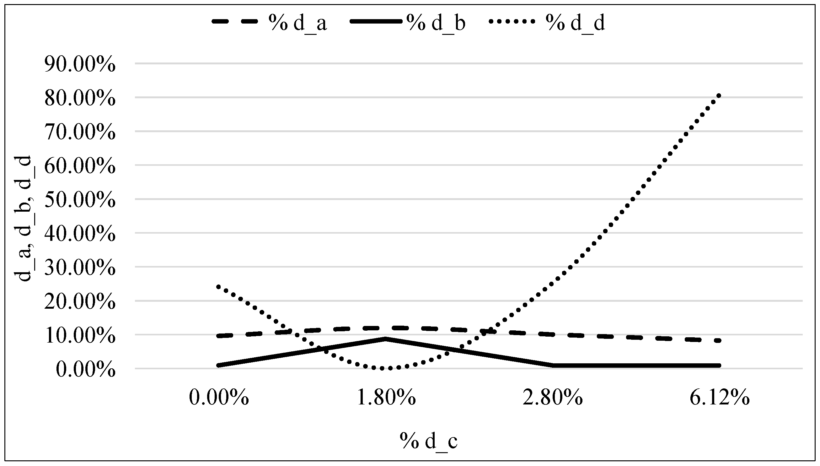
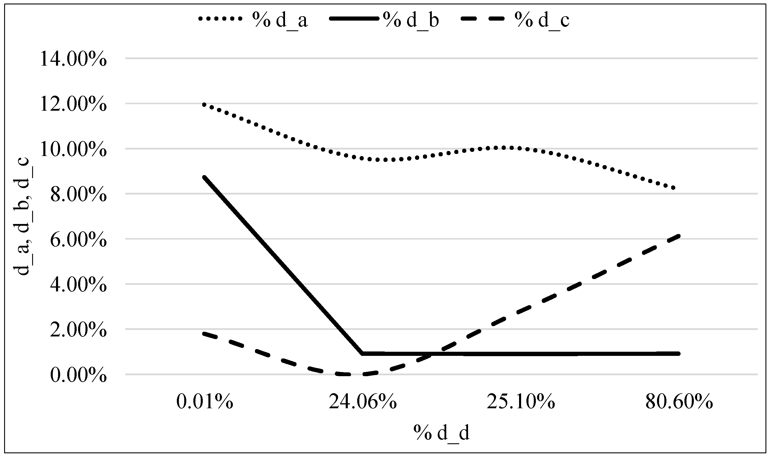
= $162,805.00), but other goals are highly deviated from their respective target values. This shows that an economical supply chain network cannot be a resilient and sustainable supply chain. Sensitivity analysis is also carried out to show the behavior of the proposed model. Figure 2 shows the percent increase in deviation of the total cost goal and its impact on the percent of deviation of the other three goals. If more importance is given to sustainability, then deviations of carbon emission and embodied carbon foot print goals tend to reduce, whereas this increases the deviation of the total cost goal ( = $189,725.40). Case II also reveals that an increment in the weightage of sustainability goals not only reduces their deviations, but also tends to reduce resilience goal deviation ( = $73,067.00). Sensitivity analysis (see Figure 3 and Figure 4) also reveals that the design of a sustainable and resilient supply chain network is less an economical network, but has the ability to achieve sustainability targets while coping with disruption risks. Case III and the sensitivity analysis in Figure 5 show that the percent of increase in the deviation of the resilience goal reduces the percent of deviation of the total cost goal. The analysis of the supply flow shows that products should be produced and transported in small quantities in high risk zones, which will reduce the impact of disruption, but increase the cost of production and transportation. This shows that an economical supply chain not only has poor sustainability, but also is highly vulnerable to disruption risks. The results of the case example reveal that firms can minimize the expected disruption cost with a small increment in the total supply chain cost. The proposed model gives many insights into the managing of sustainable supply chain networks under disruption risks, and the model provides a compromise solution by varying the supply flow between supplier, manufacturing, warehouse and customer zones, to meet different goals, as shown in Table 17., % and % with % .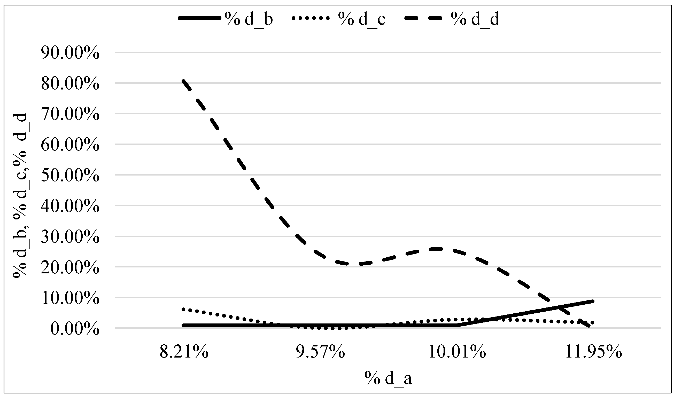 , % and % with % .
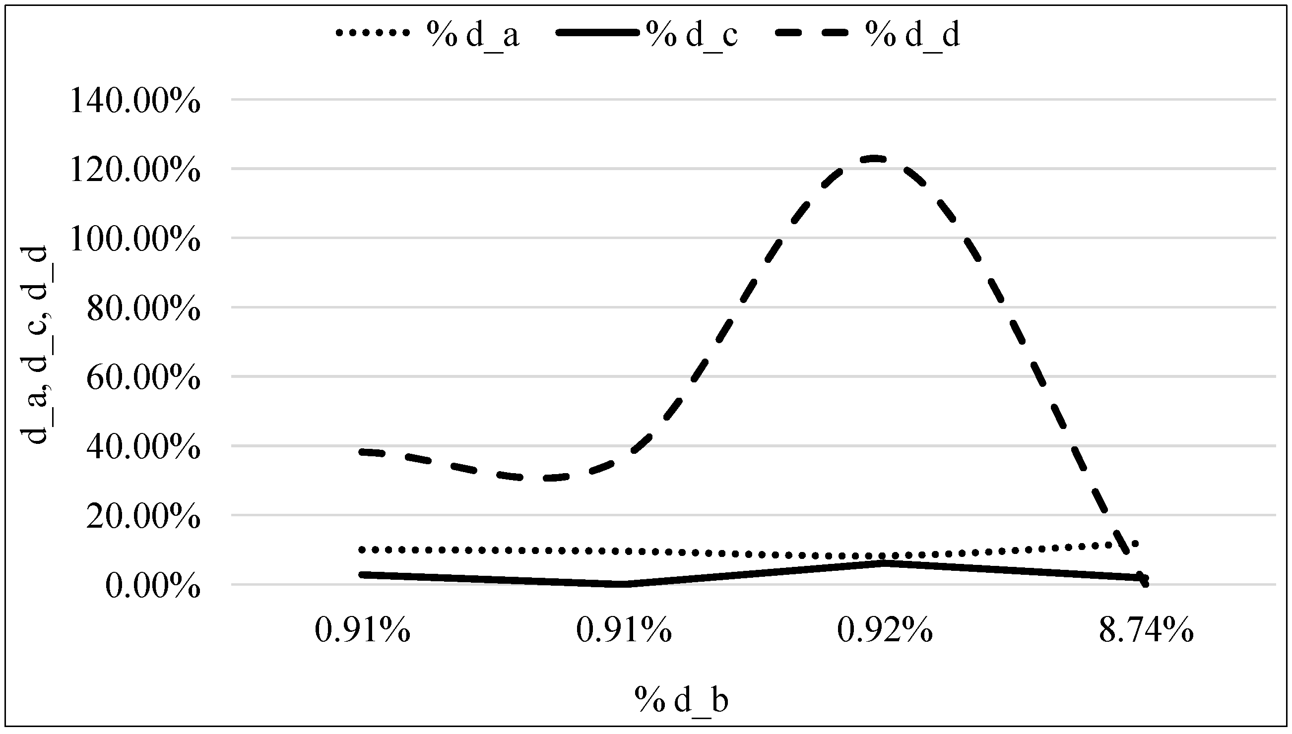 , % and % with % .
 , % and % with % .
4. Conclusions
Acknowledgments
Author Contributions
Conflicts of Interest
References
- Kumar Kundu, C. Analysis of Challenges in Existing Textile Retail Business for Implementing Sustainable Resilient Supply Chain; University of Borås: Borås, Sweden, 2010. [Google Scholar]
- Beske, P.; Seuring, S. Putting Sustainability into Supply Chain Management. Supply Chain Manag. 2014, 19, 322–331. [Google Scholar] [CrossRef]
- Elkington, J. Partnerships from cannibals with forks: The triple bottom line of 21st-century business. Environ. Q. Manag. 1998, 8, 37–51. [Google Scholar]
- Amindoust, A.; Ahmed, S.; Saghafinia, A.; Bahreininejad, A. Sustainable supplier selection: A ranking model based on fuzzy inference system. Appl. Soft Comput. 2012, 12, 1668–1677. [Google Scholar] [CrossRef]
- Choi, T.M. Optimal apparel supplier selection with forecast updates under carbon emission taxation scheme. Comput. Oper. Res. 2013, 40, 2646–2655. [Google Scholar] [CrossRef]
- Correia, F.; Howard, M.; Hawkins, B.; Pye, A.; Lamming, R. Low carbon procurement: An emerging agenda. J. Purch. Supply Manag. 2013, 19, 58–64. [Google Scholar] [CrossRef]
- Haake, H.; Seuring, S. Sustainable Procurement of Minor Items—Exploring Limits to Sustainability. Sustain. Dev. 2009, 17, 284–294. [Google Scholar] [CrossRef]
- Walker, H.; Brammer, S. Sustainable procurement in the United Kingdom public sector. Supply Chain Manag. 2009, 14, 128–137. [Google Scholar] [CrossRef]
- Nagurney, A.; Liu, Z.G.; Woolley, T. Sustainable Supply Chain and Transportation Networks. Int. J. Sustain. Transp. 2007, 1, 29–51. [Google Scholar] [CrossRef]
- Sanchez-Rodrigues, V.; Potter, A.; Naim, M.M. The impact of logistics uncertainty on sustainable transport operations. Int. J. Phys. Distr. Logist. 2010, 40, 61–83. [Google Scholar] [CrossRef]
- Tang, S.; Wang, W.; Cho, S. Reduction Carbon Emissions in Supply Chain Through Logistics Outsourcing. J. Syst. Manag. Sci. 2014, 4, 10–15. [Google Scholar]
- Sarkis, J.; Helms, M.M.; Hervani, A.A. Reverse Logistics and Social Sustainability. Corp. Soc. Responsib. Environ. Manag. 2010, 17, 337–354. [Google Scholar] [CrossRef]
- Linton, J.D.; Klassen, R.; Jayaraman, V. Sustainable supply chains: An introduction. J. Oper. Manag. 2007, 25, 1075–1082. [Google Scholar] [CrossRef]
- Paksoy, T. Optimizing a supply chain network with emission trading factor. Sci. Res. Essays 2010, 5, 2535–2546. [Google Scholar]
- Schaltegger, S.; Burritt, R.L. Measuring and Managing Sustainability Performance of Supply Chains Review and Sustainability Supply Chain Management Framework. Supply Chain Manag. An Int. J. 2014, 19, 232–241. [Google Scholar] [CrossRef]
- Shaw, K.; Shankar, R.; Yadav, S.S.; Thakur, L.S. Modeling a low-carbon garment supply chain. Prod. Plan. Control 2013, 24, 851–865. [Google Scholar] [CrossRef]
- Derissen, S.; Quaas, M.F.; Baumgärtner, S. The relationship between resilience and sustainability of ecological-economic systems. Ecol. Econ. 2011, 70, 1121–1128. [Google Scholar] [CrossRef]
- Rose, A. Resilience and sustainability in the face of disasters. Environ. Innov. Soc. Transit. 2011, 1, 96–100. [Google Scholar] [CrossRef]
- Turner, I. Vulnerability and resilience: Coalescing or paralleling approaches for sustainability science? Glob. Environ. Chang. 2010, 20, 570–576. [Google Scholar] [CrossRef]
- Lebel, L.; Anderies, J.M.; Campbell, B.; Folke, C.; Hatfield-Dodds, S.; Hughes, T.P.; Wilson, J. Governance and the capacity to manage resilience in regional social-ecological systems. Ecol. Econ. 2006, 11, 1–21. [Google Scholar]
- Perrings, C. Resilience and sustainable development. Environ. Dev. Econ. 2006, 11, 417–427. [Google Scholar] [CrossRef]
- Cutter, S.L. Building Disaster Resilience: Steps toward Sustainability. Chall. Sustain. 2013, 1, 72–79. [Google Scholar]
- De Rosa, V.; Gebhard, M.; Hartmann, E.; Wollenweber, J. Robust sustainable bi-directional logistics network design under uncertainty. Int. J. Prod. Econ. 2013, 145, 184–198. [Google Scholar] [CrossRef]
- Carvalho, H.; Azevedo, S. Trade-offs among lean, agile, resilient and green paradigms in supply chain management: A case study approach. In Proceedings of the Seventh International Conference on Management Science and Engineering Management; Springer: Berlin/Heidelberg, Germany, 2014; pp. 953–968. [Google Scholar]
- Btandon-Jones, E.; Squire, B.; Autry, C.; Petersen, K.J. A Contingent Resource-Based Perspective of Supply Chain Resilience and Robustness. J. Supply Chain Manag. 2014, 50, 55–73. [Google Scholar]
- Christopher, M.; Peck, H. Building the Resilient Supply Chain. Int. J. Logist. Manag. 2004, 15, 1–14. [Google Scholar] [CrossRef] [Green Version]
- Kristianto, Y.; Gunasekaran, A.; Helo, P.; Hao, Y. A model of resilient supply chain network design: A two-stage programming with fuzzy shortest path. Expert Syst. Appl. 2014, 41, 39–49. [Google Scholar] [CrossRef]
- Pettit, T.J. Supply Chain Resilience: Development of a Conceptual Framework, an Assessment Tool and an Implementation Process. Ph.D. Thesis, The Ohio State University, Columbus, OH, USA, 2008. [Google Scholar]
- Pettit, T.J.; Fiksel, J.; Croxton, K.L. Ensuring supply chain resilience: Development of a conceptual framework. J. Bus. Logist. 2010, 31, 1–21. [Google Scholar] [CrossRef]
- Sheffi, Y.; Closs, D.J.; Davidson, J.; French, D.; Gordon, B.; Martichenko, R.; Mentzer, J.T.; Norek, C.; Seiersen, N.; Stank, T. Supply Chain Resilience. Off. Mag. Logist. Inst. 2006, 12, 1–32. [Google Scholar]
- Shukla, A.; Lalit, V.A.; Venkatasubramanian, V. Optimizing efficiency-robustness trade-offs in supply chain design under uncertainty due to disruptions. Int. J. Phys. Distr. Logist. 2011, 41, 623–647. [Google Scholar] [CrossRef]
- Azevedo, S.G.; Govindan, K.; Carvalho, H.; Cruz-Machado, V. Ecosilient Index to assess the greenness and resilience of the upstream automotive supply chain. J. Clean. Prod. 2013, 56, 131–146. [Google Scholar] [CrossRef]
- Chang, C.T. Efficient structures of achievement functions for goal programming models. Asia Pac. J. Oper. Res. 2007, 24, 755–764. [Google Scholar] [CrossRef]
- Lim, M.K.; Bassamboo, A.; Chopra, S.; Daskin, M.S. Facility location decisions with random disruptions and imperfect estimation. Manuf. Serv. Oper. Manag. 2013, 15, 239–249. [Google Scholar]
- Chopra, S.; Sodhi, M.S. Reducing the Risk of Supply Chain Disruptions. MIT Sloan Manag. Rev. 2014, 55, 72–80. [Google Scholar]
- Klibi, W.; Martel, A.; Guitouni, A. The design of robust value-creating supply chain networks: A critical review. Eur. J. Oper. Res. 2010, 203, 283–293. [Google Scholar] [CrossRef]
© 2014 by the authors; licensee MDPI, Basel, Switzerland. This article is an open access article distributed under the terms and conditions of the Creative Commons Attribution license (http://creativecommons.org/licenses/by/4.0/).
Share and Cite
Mari, S.I.; Lee, Y.H.; Memon, M.S. Sustainable and Resilient Supply Chain Network Design under Disruption Risks. Sustainability 2014, 6, 6666-6686. https://doi.org/10.3390/su6106666
Mari SI, Lee YH, Memon MS. Sustainable and Resilient Supply Chain Network Design under Disruption Risks. Sustainability. 2014; 6(10):6666-6686. https://doi.org/10.3390/su6106666
Chicago/Turabian StyleMari, Sonia Irshad, Young Hae Lee, and Muhammad Saad Memon. 2014. "Sustainable and Resilient Supply Chain Network Design under Disruption Risks" Sustainability 6, no. 10: 6666-6686. https://doi.org/10.3390/su6106666