Inserting Ecological Detail into Economic Analysis: Agricultural Nutrient Loading of an Estuary Fishery

Abstract

Linked general equilibrium economic and ecological models are connected through agricultural runoff and the fisheries. They are applied to a North Carolina estuary in which agricultural runoff alters phytoplankton densities and the resulting hypoxia leads to diminished fisheries. The effects of hypoxia on multiple species across space are analyzed and the joint economic and ecosystem wide response to a policy of reduced runoff is quantified. The approach provides an assessment of changes in ecological welfare (in terms of species populations) and economic welfare (in terms of equivalent variations) following reductions in runoff.

1. Introduction

Much of economic modeling involves optimizing behavior by agents who interact in institutions with other optimizing agents to shape equilibrium outcomes. For example, economists postulate that consumers and producers are motivated by utility and profit, and they respond to incentives in the form of prices that are generated by their individual choices within market institutions. Of course, real people may be motivated by many factors; nevertheless, by focusing on utility and profit and assuming rational behavior economic models are useful in predicting the impact of policies on the prices, quantities, incomes and profits that follow from individual choices.

With some modification, this modeling framework applies equally well to plants and animals living in ecological systems. Individual plants and animals can be modeled as motivated by fitness. Theyrespond to incentives in the form of energy prices that are generated by their individual choices and the choices of other plants and animals within predator-prey and competitive relationships. And while plants and animals exhibit a bewildering array of strategies in the pursuit of fitness, by assuming consistent behavior, which may be less stringent than assuming rational behavior by humans, the economic modeling approach can be useful for predicting the impact of policies on plant and animal biomass demands and supplies, energy prices, and population dynamics that follow from individual choices.

Also like economies, ecosystems can be modeled in either a partial equilibrium or a general equilibrium framework. The former framework in economics requires isolating one or a few markets while fixing demands and supplies in other markets, and assuming that there are no feedback effects to those other markets from the markets under scrutiny. Similarly, in ecosystems partial equilibrium analysis requires isolating one or a few species while fixing the biomass demands and supplies of other species and assuming no feedback effects. Partial equilibrium is often adequate for understanding individual choices in isolated circumstances, although if there are important feedback effects, it can lead to seriously wrong conclusions about system wide outcomes [1,2]. Because feedbacks abound in both economies and ecosystems, there are many problems that are intrinsically general equilibrium in nature.

In this paper we take as given that integrating economics and ecology for better policy making is appropriate and desirable [3-6]. To this end, we draw upon the numerous similarities between economies and ecosystems to construct linked general equilibrium models of both systems. This approach avoids the tradition in economics of modeling ecosystems as a mere technical constraint on economic activity. The technical constraint usually is the logistic curve, and it is derived from an extreme partial-equilibrium version of an ecosystem. The curve depicts the growth of a single species while all other species are represented by a fixed carrying capacity. There is no underlying optimization by purposeful individuals, and there are no general equilibrium feedbacks. Such models miss the entire biological nature of nature.

Economic management policies derived from single species models inevitably will generate impacts on many other species in the ecosystem. These impacts move the ecosystem to a different equilibrium that may be an unintended consequence of the policy, thereby generating ecosystem externalities in the economy [7]. Moreover, people have demonstrated time and again that they have preferences about ecosystem externalities; that is, they are concerned not only with the policy goals but with the process that leads to the goals. “Because economic values depend on individuals' own assessments of their well-being, an understanding of the ways in which specific impairments of an ecosystem diminish their lives is essential.” [5] (p. 1388). Examples of such impairments are: the loss of cultural ecosystem services when bison that wander out of the Yellowstone Park on snowmobile trails are culled, the loss of marine ecosystem diversity when forage fish are harvested to feed hatchery salmon, and economic growth leading to the loss of charismatic birds and the cultural and supporting ecosystem services they provide [8]. Without a model that describes species interactions, one may miss different types of interactions between people and the ecosystem, because one cannot trace the ecosystem externalities that create the impairments.

Our linked general equilibrium approach describes the relationship between parallel, linked adaptive systems [9-11]. It is applied to a North Carolina estuary in which agricultural runoff altersphytoplankton densities and the resulting hypoxia leads to diminished fisheries. The general equilibrium economic model and the general equilibrium ecological model are connected through agricultural runoff and the fisheries, and important issues that are addressed include: (i) the choice of compatible spatial and temporal scales across the two systems; (ii) the role of dynamics; (iii) the boundaries of the systems and how entry and exit of firms and species occurs; and (iv) what outcomes from the systems are important and how they can be measured. The effects of hypoxia on multiple species across space are analyzed and the joint economic and ecosystem wide response to a policy of reduced runoff is quantified. The approach provides an assessment of changes in ecological welfare (in terms of species populations) and economic welfare (in terms of equivalent variations) following reductions in runoff. After developing the general equilibrium models, we highlight the advantages of a linked approach.

2. The General Equilibrium Ecosystem Model (GEEM)

GEEM combines two disparate ecological modeling approaches: optimum foraging models and dynamic population models. The former approach has been likened to consumer theory [12] and describes how individual predators search for, attack and handle prey to maximize net energy intake per unit time. The approach does not account for multiple species in complex food webs and it does not track species population changes. The latter approach tracks population changes by using a difference or differential equation for each species. The familiar logistic-growth model used extensively in the economics literature is the simplest example, although extensions include resource competition models, e.g., [13], and multi-species models, for example, [14-22]. However, the parameters in the dynamic equations represent species-level aggregate behavior: optimization by individual plants or animals or by the species is absent. Alternatively, GEEM employs optimization at the individual level as in foraging models, and uses the results of the optimization to develop difference equations that track population changes.

GEEM also differs from large simulation models, e.g., [23,24]. First, its basic unit is an individual organism and not a species, and decisions are made by the individual. Second, it recognizes that natural selection requires plants and animals to maximize their net energy flows; thus an optimization approach is used to capture efficient energy use by all individuals. Third, species' population update equations are derived from individual behavior and linked to individual energy efficiency. Estimates of lumped parameters in the update equations are not needed.

In sum, GEEM combines general equilibrium calculations, similar to those used in Computable General Equilibrium (CGE) economic models, with dynamic population updating used in ecology. By tracking multiple populations GEEM is a step toward ecosystem-based management in which the importance of non-target species is recognized and preserving biodiversity is a goal [25].

Applying GEEM is an exercise similar to applying a basic CGE model. CGE models translate an economy into a mathematical formulation. While there are numerous methods of approaching the problem, the most common method uses individual optimization problems of firms and consumers to derive demand and supply functions. These functions describe how these agents react to prices and perturbations in other variables, and they are used to construct the equilibrium conditions of the model. Thus the problem is converted to solving a square system of equations, where optimal individual behaviors are embedded in the system. The numerical solution finds values of endogenous variablesfor given values of exogenous parameters. Endogenous variables include outputs, prices, and demands, while exogenous parameters include preferences, technologies, and factor endowments.

The initial data for a CGE is usually represented by a rectangular matrix known as a social accounting matrix (SAM). A SAM basically broadens a traditional input-output table to encapsulate all monetary and real flows in an economy. SAMs present what is assumed to be an observed equilibrium for an economy, and provide a tabular description of the circular flows of commodities and money throughout an economy. They display all the consumer and firm receipts and expenditures, with the requirement that in equilibrium receipts and expenditures balance.

Before running a CGE model a validity test is conducted in which the CGE is required to replicate the SAM equilibrium. To find parameters that are not available in the initial data, the SAM benchmark endogenous variables are used to calibrate the model to the observed equilibrium. Following calibration the CGE is run using the parameters and it is validated if it replicates the SAM.

GEEM also uses individual optimization problems to derive demand and supply functions, although the individuals are plants and animals who are maximizing their net energy devoted to reproduction. Quantities are in biomass units and prices are in energy units: for example, a predator expends energy to capture and consume prey biomass. As with CGE, the numerical solution finds values of endogenous variables for given values of exogenous parameters. Endogenous variables include biomass demands and supplies and energy prices, while exogenous parameters include individuals' respiration and predation parameters, weights, embodied energies and species populations.

Initial data is needed for GEEM that may be labeled an ecological accounting matrix (EAM). EAMs provide what is assumed to be an observed equilibrium for an ecosystem, and provide a tabular description of the circular flows of biomass and energy throughout an ecosystem. They display all the plant and animal biomass receipts and energy expenditures, with the requirement that in equilibrium receipts and expenditures balance. Again as with CGE, a validity test is conducted wherein the EAM is assumed to be an observed equilibrium and GEEM is required to replicate this equilibrium.

Where GEEM departs from CGE is in tracking the species populations. That is, in CGE the numbers of consumers or firms are exogenous, but treating species populations as exogenous would miss what may be the most important characteristic of the ecosystem—how populations are changing over time. To determine population changes, after each general equilibrium calculation, the individuals' optimum net energies are used to update the populations. Therefore, populations are exogenous for each general equilibrium calculation but endogenous over time, and GEEM should be thought of as a series of general equilibrium calculations in which the numbers of individuals are changing between calculations. If the numbers of individuals cease to change, then a steady state is said to be attained.

2.1. The Structure of GEEM in the Neuse

The Food Web

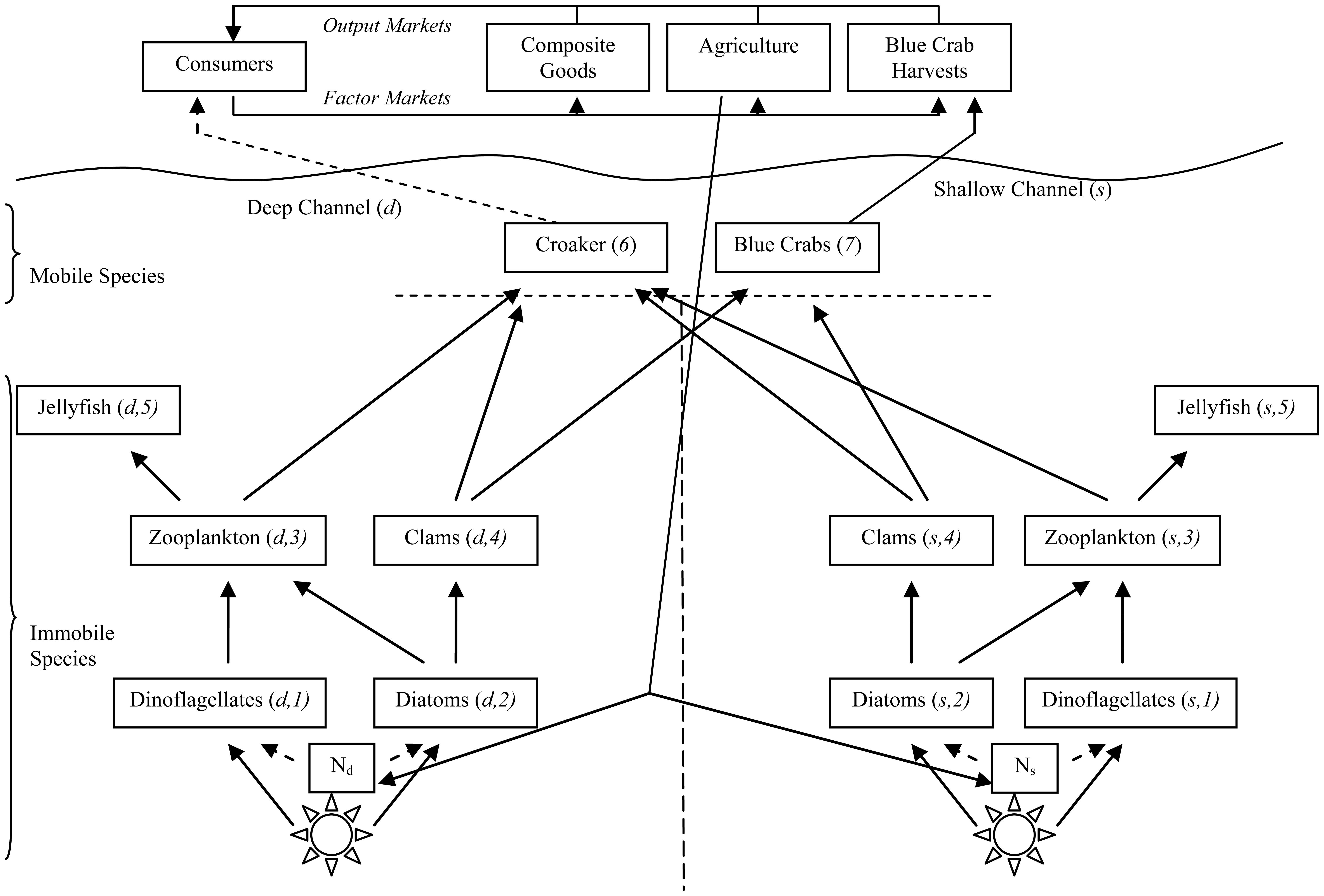
In the estuarine ecosystem divided into deep and shallow channels, all energy originates from the sun and it is turned into biomass through photosynthesis by various species of algae and phytoplankton that are aggregated into two species: diatoms and dinoflagellates. All individual animals depend either directly or indirectly on these phytoplankton. The simplified food web in Figure 1 loosely follows those presented in [26-29] although it is extended to include the spatialimportance of deep and shallow channels of hypoxia in the main channel. Species in Figure 1 are numbered 1–7.

In deep and shallow channels, individuals of lower species are immobile. Dinoflagellates are viewed as nuisance phytoplankton as they bloom with elevated N loading and eventually lead to hypoxic conditions. Dinoflagellates are able to out-compete the diatom phytoplankton for access to solar energy under elevated N levels. Dinoflagellates have lower energy content than the diatoms, ceteris paribus making them less desirable prey. Dinoflagellate blooms result in increased sediment oxygen demand (SOD) as bacteria consume dead dinoflagellates. In turn, increased SOD means decreased dissolved oxygen (DO) that is detrimental to marine animals.

The next trophic level of immobile individuals are aggregated zooplankton (copepods) and bivalve (clam) species (Macoma balthica, Macoma bitchelli, and Mulinia bateralis). Zooplankton prey on both dinoflagellates and diatoms, while clams only target diatoms. Jellyfish (Chrysoara quinquechirra and Mnemiopsis leidyi) round out the immobile species in both channels, and they only consume zooplankton.

Croaker (Micropogonias undulatus) and blue crabs (Callinectes sapidus) migrate between deep and shallow channels. Croaker prey on zooplankton and clams in both channels, while blue crabs target only clams in both channels.

GEEM Equations

There are three sets of equations in GEEM, the individual plant and animal objective functions, the demand/supply clearing conditions, one for each predator/prey relationship, and the population update equations, one for each species. The first two sets of equations comprise the general equilibrium calculations that are carried out for current species populations. The third set of equations employ the calculations to update the populations that are then used in next period's general equilibrium calculations.

Consider the blue crab objective function in the absence of anthropogenic intervention:

$$R_7=\mathit{[}{e}_4-e_{74}^d\mathit{]}{x}_{74}^d+\mathit{[}{e}_4-e_{74}^s\mathit{]}{x}_{74}^s-f_7\mathit{(}{x}_{74}^d,x_{74}^s\mathit{)}-{\beta }_7$$

(2.1)

R7 is net energy in power units (e.g., Watts) [30-34]. The numerical subscripts are species indices from Figure 1. The first two terms on the right side are the inflow of energies from deep (d) and shallow (s) clams. The choice variables, $x_{74}^w,w=d,s$, are the biomasses (milligrams year ⁻¹) transferred from clams in channel w to the blue crab, e₄ is the energy (joules mg⁻¹) embodied in clam biomass, and $e_{74}^w,w=d,s$, are the energies (J mg⁻¹) the blue crab expends to locate, capture and handle clam biomass. These latter energies are the energy prices and the blue crab's choice of prey will depend on relative energy prices. Blue crab individuals are assumed to be price takers because each is only one among many individuals in a predator species capturing one of many individuals in a prey species. However, within the ecosystem the prices are endogenous, being determined by demand and supply.

The third and fourth terms in Equation (2.1) represent respiration energy allocated to growth and maintenance, or to reproduction as explained in the dynamics. Following [13] respiration is divided into a variable part f₇(·) that depends on biomass intake, and a fixed part β₇ that is basal metabolism. We use a quadratic form for variable respiration that allows continuous substitution among prey species:

$$f_7\mathit{(}{x}_{74}^d,x_{74}^s\mathit{)}={\alpha }_4\mathit{(}{x}_{74}^d,x_{74}^s\mathit{)}+.5{\alpha }_4\mathit{(}{x}_{74}^d{x}_{74}^s+{x_{74}^d}^2+{x_{74}^s}^2\mathit{)}$$

(2.2)

where α4 is a parameter determined in calibration as explained below.

The objective function for an individual in a prey species has additional terms for predation. Consider a clam in the deep channel:

$$R_4=\mathit{[}{e}_2-e_{42}^d\mathit{]}{x}_{42}^d-f_7\mathit{(}{x}_{42}^d\mathit{)}-{\beta }_4-d_{46}{e}_4\mathit{(}1+t_{64}{e}_{64}\mathit{)}{x_{42}^d}^{1/2}-d_{47}{e}_4\mathit{(}1+t_{74}{e}_{74}\mathit{)}{x_{42}^d}^{1/2}$$

(2.3)

The first three terms are comparable to the blue crab Equation (2.1) except that the clam has diatoms as its sole prey. The last two terms are energies lost by the clam to croaker and blue crab predation. Looking at the fourth term, the more diatom biomass a clam captures the more it is exposed to predation and the more biomass it supplies to croakers. This tradeoff between foraging gains and losses is called predation risk [35], and it permits the biomass the clam supplies to croaker to be a function of clam demand for diatoms. This representation is similar to, but in reverse from, a firm whose supply of output determines its demand for inputs. The d₄₆ is a parameter obtained from calibration and e₄ is the embodied energy in a clam. The term in parentheses represents the predation risk. It is assumed to be a linear function of the energy the croaker use in capture attempts, e₆₄. The more energy croaker expend, the more energy the clam expends escaping. In a sense, t₆₄ is a tax on the clam because it loses energy above what it loses owing to being captured [36]. The functional form of the predation term is consistent with expected population movements [34].

Assuming second-order sufficient conditions for a maximum are satisfied [34], the first-order conditions from maximizing Equations (2.1) and (2.3) and comparable first-order conditions for croaker, and deep and shallow jellyfish, zooplankton, diatoms and dinoflegellates, can be solved for the x_ij as functions of the energy prices to yield biomass demand of an individual in species i for species j:

$$x_{ij}^w\mathit{(}\overline{e}\mathit{)}$$

(2.4)

and biomass supply of an individual in species i to species k using (2.3):

$$y_{ik}\mathit{(}{x}_{ij}^w\mathit{(}\overline{e}\mathit{)}\mathit{)}=d_{ik}{x_{ij}^w}^{1/2}$$

(2.5)

The ē is a vector of all energy prices, w = d, s, and the i, j and k are from the predator and prey indices in Figure 1.

The second set of equations used in the general equilibrium calculations is comparable to market clearing equations in CGE. To find a set of energy prices that equate demands and supplies, an equilibrium equation is needed for each price. Because each animal and plant is assumed to be a representative individual from its species, all organisms in each species are identical; therefore, the demand and supply sums are obtained by multiplying the representative individual's demands and supplies by the species populations. Letting n_i be the population of species i, the equilibrium conditions take the form:

$$n_i{x}_{ij}^k\mathit{(}\overline{e}\mathit{)}=n_j{y}_{ij}\mathit{(}{x}_{jk}^w\mathit{(}\overline{e}\mathit{)}\mathit{)}$$

(2.6)

There is one condition for each biomass transfer. The left side of Equation (2.6) is the total demand of species i for species j, and the right side is the total supply of species j to species i where species j preys on species k [37].

The third set of equations in GEEM update the populations. To be consistent with the CGE calculations, time in the ecosystem is divided into years and species reproduce each year. In reality, all species other than croaker reproduce in the estuary at least twice a year, lower level species many times per year. For simplicity, the following presentation of the update equations assume one year reproductive cycles, but in the calculations lifespans and weights used in the population adjustment equations below are modified to account for multiple cycles [38].

A representative plant or animal may have positive, zero or negative net energy in the general equilibrium calculations. Positive (zero, negative) net energy is associated with greater (constant, lesser) fitness and an increasing (constant, decreasing) population between periods. (The analogy in a competitive economy is the number of firms in an industry changes according to the sign of profits.) Net energies, therefore, are the source of dynamic adjustments. If the period-by-period adjustments drive the net energies to zero, the system attains a steady state. The predator/prey responses to changing energy prices tend to move the system to steady state.

Consider population changes for top predator species i. In steady-state it must be the case that births equals deaths. If s_i is the lifespan of the representative individual, then the total number of births and deaths must be n_i/s_i, with per capita steady-state birth and death rates of 1/s_i. The top predator's maximized net energy is given by R_i(x_ij; n^t) = R_i (·) which is obtained by substituting the optimum demands as functions of energy prices into (2.1). N^t is a vector of all species populations and it indicates that net energy in time period t depends on all populations in time period t. In the steady state, R_i(·) = 0. Reproduction requires energy and, by the definitions of the terms in Equation (2.1), some o that energy is contained in the variable respiration. Let v_i^ss be the steady-state variable respiration, and let ${\rho }_i{\nu }_i^{ss}$ be the proportion of this variable respiration devoted to reproduction. Thus, in steady state the energy given by ${\rho }_i{\nu }_i^{ss}$ over all members of the species yields the number of births that exactly offset deaths:

$$\text{births}=\text{deaths}==>n_i^{ss}{\rho }_i{\nu }_i^{ss}=n_i^{ss}(1/s_i)$$

The term ${\rho }_i=\left(1/{\nu }_i^{ss}{s}_i\right)$ found from this relationship converts reproductive energy into individuals.

Next, suppose the top predator is not in steady state and that R (·) ≠ 0 and variable respiration is v_i. Assuming that the proportion of R_i (·)that is available for reproduction is the same as the proportion of variable respiration available for reproduction, the energy now available for reproduction is ρ_i [R_i (·) + v_i]. Assuming that reproduction is linear in available energy, then it follows that if ${\rho }_i{\nu }_i^{ss}$ yields a per capita birth rate 1/s_i, then ρ_i [R_i (·) + v_i] yields a per capita birth rate of $\frac{1}{s_i{\nu }_i^{ss}}[R_i(.)+{\nu }_i]$.

The change in population is obtained by multiplying the population by the difference between the birth and death rates, where the latter rate is assumed independent of energy available for reproduction. Therefore the population adjustment equation is:

$$n_i^{t+1}=n_i^t+n_i^t\left[\frac{[R_i(.)+{\nu }_i]}{s_i{\nu }_i^{ss}}-\frac{1}{s_i}\right]$$

(2.7)

Expression (2.7) reduces to the steady state if R_i(·) = 0 (in which case ${\text{v}}_i={\text{v}}_i^{ss}$ and $n_i^{t+1}=n_i^t$). Because the biomass demands depend on the period t populations of all species, the population adjustment for species i depends on the populations of all other species. In addition, out of steady state R_i (·) and v_i change across periods. These changes distinguish the GEEM approach from most all ecological dynamic population models, because the latter rely on fixed parameters in the adjustment equations that do not respond to changing ecosystem conditions.

If the species is not a top predator but is prey for another species, then in steady state the births must equal the deaths plus any individuals lost to predation. From Equation (2.5), each individual loses $y_{ij}\mathit{(}{x}_{ij}^w\mathit{(}\overline{e}\mathit{)}\mathit{)}=d_{ij}{x_{ij}^w}^{1/2}$ of biomass to predator k. The summation of all individual losses to predation gives the total biomass lost, and dividing by weight of a representative individual provides the number of individuals lost to predation:

$$n_i^t{y}_{ij}\mathit{(}{x}_{jk}^w\mathit{(}\overline{e}\mathit{)}\mathit{)}/w_i$$

(2.8)

Thus, in steady state, the number of births from respiration energy, equals the sum of deaths from predation and deaths from natural mortality net of losses to predation:

$$n_i^{ss}{\rho }_i{\nu }_i^{ss}=n_i^{ss}\left[\frac{y_{ik}(x_{ij}^w(\overline{e}))}{w_i}\left(1-\left(1/s_i\right)\right)+\left(1/s_i\right)\right]$$

(2.9)

The parameter ρ_i can again be found from this relationship although now it includes predation and natural mortality:

$${\rho }_i=\left(\frac{\left(y_{ik}\left(x_{ij}^w(\overline{e})/w_i\right)(1-(1/s_i))+(1/s_i)\right)}{{\nu }_i^{ss}}\right)$$

(2.10)

Again, assuming that the proportion of R_i (·) available for reproduction is the same as the proportion of variable respiration available for reproduction, when the species is not in the steady state the population update function becomes:

$$n_i^{t+1}=n_i^t+n_i^t\left[\frac{y_{ik}\mathit{(}{x}_{ij}^w\mathit{(}\overline{e}\mathit{)}\mathit{)}}{w_i}\left(1-\frac{1}{s_i}\right)+\left(\frac{1}{s_i}\right)\right]\left[\frac{(R_i(.)+{\nu }_i)}{{\nu }_i^{ss}}-1\right]$$

(2.11)

In steady state R_i(·) = 0, v_i = v_i^ss and (2.11) reduces to $n_i^{t+1}=n_i^t$.

2.2. Nutrient Loading and Phytoplankton

Hypoxia

Tilman [39-41] developed the resource-ratio hypothesis that underscores the importance of limiting resources for explaining community structure. The importance of N flows into ecosystem health is admitted to GEEM through the phytoplankton maximization problems. We assume that when a plant is stressed by a shortage or surplus of N, the plant will require additional energy for any biomass it produces [42]. Thus, there is an optimum level of N for each plant and movements away from the optimum increase respiration energy losses. This is in contrast to introducing the influence of a resource into a lumped parameter population adjustment equation [43,44].

Write the objective function for a representative deep-channel dinoflagellate as:

$$R_1=\mathit{[}e-e_0^d\mathit{]}{a}_1{x}_{10}^d-f_1\mathit{(}{x}_{10}^d\mathit{)}-{\beta }_1-d_{13}{e}_1\mathit{(}1+t_{13}{e}_{31}\mathit{)}{x_{10}^d}^{1/2}$$

(2.12)

The first term is incoming energy, the second and third terms are variable and fixed respiration, and the last term is predation energy losses to zooplankton. There are differences between a plant and animal objective function that deserve mention. The choice variable x₁₀ is the plant's biomass (mg): other things equal, the greater the biomass the greater the exposure to light energy. The (J time cm) is the flow of both direct and indirect solar radiation arriving at the surface of the plant for each unit of area. The a_i (cm² mg⁻¹) is the plant s specific leaf area (SLA) or the area covered by a plant's biomass. SLA can vary by an order of magnitude across terrestrial species [45]. Here the a_i is species specific and assumed constant. While the specifics of the terminology may not be appropriate for aquatic plants, the general processes for aquatic plants are assumed to be consistent with those of terrestrial plants. The $e_0^d$ (J time⁻¹ mg⁻¹) is the deep channel congestion energy loss (CEL). Because of mutual shading, plants incur this loss in competing for access to light. The CEL is like an economic price that competing firms pay for an input: each plant takes CEL as a parameter in its optimization problem, and it is determined by a “market” clearing condition, see [37]. Both dinoflagellates and diatoms must “pay” this same CEL as they compete for the same space [46].

N enters in the variable respiration function from Equation (2.12):

$$f_1\mathit{(}{x}_{10},N\mathit{)}={\alpha }_1{x}_{10}^2\left({(N-N_1)}^2+1\right)$$

(2.13)

The parameter a₁ (J time⁻¹ mm⁻²) converts the plant s biomass to respiration and is determined in the calibration. The N₁ is dinoflagellate's ideal level of N, and when N = N₁ the plant's variable respiration is at a minimum for a given biomass. When N ≠ N_i, N differs from the ideal and the plant is stressed via increased respiration. Adding N to the plant maximization problem makes plant growth rates and steady-state sizes a function of a time-dependent environmental factor as in [47]. Dinoflagellates have a population update equations like Equation (2.11), and diatoms are treated similar to dinoflagellates.

Oxygen Depletion

To link N flows and phytoplankton perturbations with SOD, DO, and animal respiration, a multiple-step procedure is employed [48]. First, phytoplankton blooms are linked to SOD following [49]. The method calculates an elasticity of SOD to dinoflagellate biomass, ${\mathit{\varepsilon }}_{n_1}^{\mathit{\text{SOD}}}$, from the derivation of SOD provided in [50,51]. The value ${\mathit{\varepsilon }}_{n_1}^{\mathit{\text{SOD}}}=0.7071$ was calculated using Neuse data. DO is assumed to respond perfectly to changes in SOD so that the elasticity of DO to changes in dinoflagellate biomass is inferred to be ${\mathit{\varepsilon }}_{n_1}^{OD}=-0.7071$.

Second, DO changes are related to stress on animal species. Studies exist that show reduced DO lead to increased, non predatory mortality although a study specific to the Neuse only address clams and SOD [52]. Borsuk et al. [52] calculate mean survival probabilities for various reductions in SOD. Employing their results it is possible to estimate the elasticity of clam mortality with respect to SOD, ${\mathit{\varepsilon }}_{\mathit{\text{SOD}}}^M=0.7592$ [53].

Third, we assume that the stress from low DO implies that a clam will lose additional respiration energy for any biomass it demands. Moreover, because DO is the negative of SOD, SOD can be used directly in the respiration expression. Letting the change in dinoflagellate biomass be denoted ${\Delta }^{n_1}$ the variable clam respiration energy from Equation (2.3) is written as:

$$f_7(x_{42}^d)=\left(1+{\Delta }^{n_1}{\mathit{\varepsilon }}_{n_1}^{\mathit{\text{SOD}}}{\mathit{\varepsilon }}_{\mathit{\text{SOD}}}^M\right){\alpha }_4{x_{42}^d}^2$$

(2.14)

Basically, clam variable respiration is increased by the percentage change in mortality that follows from nutrient loading. In the absence of species specific mortality studies for croaker and blue crab, the value of ${\mathit{\varepsilon }}_{\mathit{\text{SOD}}}^M$ is assumed to be the same for them and

$${\Omega }^{\text{w}}=\left(1+{\Delta }^{n_1}{\mathit{\varepsilon }}_{n_1}^{\mathit{\text{SOD}}}{\mathit{\varepsilon }}_{\mathit{\text{SOD}}}^M\right)$$

(2.15)

is appended to the croaker and blue crab variable respiration functions. In Equation (2.15), w = d, s to indicate that the stress from depleted O₂ can be different in the two channels.

2.3. Spatial Migration between Channels

Croaker and blue crab mobility between channels follows from their prey choice and hypoxic stress, with no additional mobility costs other than those associated with predation and respiration. At any time, croaker and blue crab may inhabit both regions in varying degrees as they pursue prey and avoid hypoxia. (Mistiaen et al. [54] examine the link between the blue crab fishery and DO in the Chesapeake Bay.)

Consider the blue crab objective function Equations (2.1) with (2.2) and (2.15) substituted in:

$$R_7=[e_4-e_{74}^d]x_{74}^d+[e_4-e_{74}^s]x_{74}^s-{\alpha }_4({\Omega }^d{x}_{74}^d+{\Omega }^s{x}_{74}^s)-.5{\alpha }_4({\Omega }^d{x}_{74}^d{\Omega }^s{x}_{74}^s+{\Omega }^d{x_{74}^d}^2+{\Omega }^s{x_{74}^s}^2)-{\beta }_7$$

(2.16)

A blue crab chooses the proportions of clams to consume in both channels based on the relative energy prices, $x_{74}^w$, and on the hypoxic conditions, Ω^w. At the same time the clams are stressed by O₂ depletion and they prey on diatoms whose populations are diminished by N loading. The first order condition for the blue crab's deep channel consumption is:

$$\frac{\partial R_7}{\partial x_{74}^d}=[e_4-e_{74}^d]-{\alpha }_4({\Omega }^d{x}_{74}^d)-.5{\alpha }_4({\Omega }^d{\Omega }^s{x}_{74}^s+2{\Omega }^d{x}_{74}^d)=0$$

(2.17)

An increase in the deep channel energy price, $e_{74}^d$, owing to blue crab competition for clams, or smaller clam populations brought about by hypoxia, or population changes elsewhere in the food web, lowers the marginal benefits of predation in the deep channel, and the blue crab will prey more in the shallow channel. Similarly, reductions in O₂ levels in the deep channel raises the marginal respiration cost of preying there, and again the blue crab will prey more in the shallow channel. The “jointness” in the functional form of respiration results in a direct effect from O₂ depletion on marginal cost from predation in the deep channel, and an indirect effect on the marginal cost from predation in the shallow channel.

3. The Computable General Equilibrium Model (CGE)

The North Carolina economy is described by a closed CGE model of an economy with a fishery sector. The “closed economy” assumptions of all economic production and consumption taking place within North Carolina allows a focus on the impacts of the policy throughout the North Carolina and the Neuse ecosystem. But these assumptions have consequences on the results as they neglect any responses of the greater economic and ecological systems surrounding North Carolina and the Neuse.

Within the economy, all agents are assumed to be perfectly myopic, consistent with open access in blue crab harvesting, and all savings and investment behavior omitted such that factor stocks remain constant over time. Government is included in the model only through command and control N emissions practices.

The economy has three production sectors: the blue crab fishery B, agriculture A, and composite goods C. Profit-maximizing, price-taking firms employ harvests of blue crabs in the fishery, and capital and labor in all sectors, to produce their outputs in a continuous, nonreversible, and bounded process. Outputs from the fishery, agriculture, and composite goods are sold in closed regional marketsto regional households. Capital K and labor L are homogeneous and defined in service units per period. They are also perfectly mobile between sectors and between periods. Sector i factor employment levels are given by K_i and L_i (i = B, A, C).

In simulations, commodity prices, final demands, factor employments, factor rewards, consumer incomes, species populations and harvests are endogenously determined. Changes in these variables and welfare measures are observed as N loadings are reduced. The general methods employed in the CGE model follow [55-57]. Only unique features of the methods employed are presented in detail, standard features relegated to the Appendix. Unique components of the model are the treatment of the fishery sector and agricultural costs of a N reduction policy. The blue crab fishery adapts the bioeconomics of [15] to the CGE framework following [58].

Incorporating a fishery into a CGE framework raises issues that require modifications to the standard fishery models. First, where most of the fishery literature employs effort as the single human factor of production [59,60], capital and labor must be included in CGE so that the fishery interacts with other sectors. Second, the non fishery sectors hire capital and labor in service units per time period, in this case one year, but in the fishery factors may be employed considerably less than one year. Third, harvests are spatially distinct which requires further modifications to the fishery.

To include these modifications in the CGE framework we use a nesting structure. Aggregate (non-spatially explicit) industry behavior is summarized by expressions (3.1) and (3.2):

$$H_B=d_B{T}^{{\alpha }_B}{n}_7^{{\beta }_B}$$

(3.1)

$$\begin{array}{ll}\text{minimize}W{L}_B+R{K}_B\text{subject to}\hfill & T={\varphi }_B{\left[{\delta }_B{L_B}^{{\rho }_B}+\left(1-{\delta }_B\right){K_B}^{{\rho }_B}\right]}^{1/{\rho }_B}\hfill \end{array}$$

(3.2)

Equation (3.1) introduces aggregate harvests H_B as a function of fishing season length T, the aggregate (non-spatially differentiated) blue crab population n₇, and parameters d_B, a_B, and β_B. The season length is simply an aggregate measure of effort (given by capital and labor employed in the fishery) translated into the time (days) needed to land H_B given the blue crab stock. The industry is assumed to minimize the cost of harvesting according to Equation (3.2) by employing capital and labor to work time T, at wage W and rental rate of capital R subject to the constant returns to scale aggregation function. ϕ_B and δ_B are parameters and σ_B =1/(1 − ρ_B) is the elasticity of substitution between capital and labor in the fishery. The associated cost function is linearly homogenous in time, allowing the total costs of harvesting to be written as C(W, R)T.

Spatial targeting by harvesters is introduced by defining harvests as a function of spatially delineated stocks and seasons, that balance aggregate harvest and seasons, and exhaust all rents under open access. Space in the fishery is defined by the populations of blue crab (n^d₇ and n^s₇) in the deep and shallow channels, and season lengths (T^d and T^s) required to land harvests (H^d_B and H^s_B) in either channel. Harvests and time spent harvesting in each region are given by expressions (3.3).

$$\begin{array}{c}{H}_B^d=d_B{T}^{d^{{\alpha }_B}}{n}_7^{d^{{\beta }_B}}\text{and}{H}_B^s=d_B{T}^{s^{{\alpha }_B}}{n}_7^{s^{{\beta }_B}}\\ H_B=H_B^s+H_B^d\text{and}T=T^s+T^d\end{array}$$

(3.3)

Given aggregate harvests and season lengths, spatial targeting is defined by adjustments in channel specific seasons so that there are zero net returns at the aggregate (fishery) level.

Fishery rents are driven to zero in the long-run through entry and exit of firms (in this representation given by changes in the season length). Each firm minimizes costs and applying Shepard's Lemma yields factor demands. Industry equilibrium is given by rent exhaustion:

$${\pi }_B=P_B\left(H_B^d+H_B^s\right)-C(W,R)T=0$$

(3.4)

The total factor payments over the season equal the total revenue divided by the season length, or average revenue per time. Harvesters, therefore, hire capital and labor optimally but under conditions of open access will continue to harvest (i.e., spend time harvesting) until all rents are exhausted (there is not an optimization problem for T, it is determined by rent exhaustion). We do not consider what factors employed in the fishery do during the off-season as in [58].

Standard methods are employed for agriculture, composite goods production and households, documented in the Appendix. Only the treatment of consequences from N reduction on agriculture is mentioned here. While the direct consequences on agricultural production from policies of N reductions are complex and beyond the scope of this analysis, a brute force tact is followed herein, where N reduction policies serve to increase producers' costs. This simplistic restriction allows a menu of potential cost scenarios to be seamlessly compared without having to change the technological specification of the sector. The addition of agricultural cost “shifters” modifies the industry's cost function:

$$C_A={\left({\phi }_A^N\right)}^{-1}{Q}_A{\left[{\delta }_A^{{\sigma }_A}{W}_A^{1-{\sigma }_A}+{(1-{\delta }_A)}^{{\sigma }_A}{R}_A^{1-{\sigma }_A}\right]}^{1/(1-{\sigma }_A)}$$

(3.5)

N reduction policies increase agriculture's cost function through the specification of the parameter ${\left({\varphi }_A^N\right)}^{-1}={\Delta }^N{\left({\varphi }_A\right)}^{-1}$ where Δ^N is the percentage change in agricultural costs induced by the policy and ϕ_A is the sector's efficiency parameter in the absence of any cost impacts.

Regional households derive their income from sales of labor and capital endowments and consume regional agricultural goods, composite goods and blue crab harvests. Non-market linkages between households and the ecosystem are not considered herein but remain a focus of future work. Welfare impacts of alternative policies are evaluated in terms of modified Hicksian equivalent variational measures similar to those developed in [56]. Each policy change leads to changes across prices and income in relation to a reference/benchmark sequence of business as usual. Let the Hicksian expenditure function associated with consumption in period t be given by M_t(·). Vectors of prices in any period t of the reference scenario b or policy alternate a are given by P̄^b_t and P̄^a_t, with corresponding indirect utility functions $V_t^b$ and $V_t^a$ both a function of the croaker population in that period. In the results we employ annual equivalent variations $E{V}_t=M_t\left({\overline{P}}_t^b,V_t^a\right)-M_t\left({\overline{P}}_t^b,V_t^b\right)$ (see [61]) to calculate welfare changes for every period across policy scenarios. Cumulative aggregate welfare measures are found using discounted summations of EV_t which is possible as the measure is based upon a common baseline price vector. Also, given the exogenous time horizon a termination term is added to account for welfare impacts after the final period T. In this we assume that by T the economy is close to a steady state.

4. Application to the Neuse River Estuary—Parameterization

Time is defined in annual increments, and given the small share of the North Carolina economy comprised by Neuse agriculture and blue crab harvests (less than 0.1% of state gross product), capital and labor stocks are taken as constant over time. While lacking in detail, this format allows a representation of the relative importance to the North Carolina economy of those sectors and linkages with direct contact to the Neuse.

Human generated N flows in the deep and shallow channels are spatially differentiated, distributed randomly, and taken as exogenous to the ecological model. Changes in these inputs impact the resource competition between dinoflagellates and diatoms, with resulting energy transfer impacts up the food web. As described below, dinoflagellates are assumed to prosper at higher levels of N, while diatoms prosper at lower levels.

Ecological data for the Neuse estuary were obtained for plant and animal populations, benchmark plant biomasses and animal biomass demands, and parameters that include embodied energies, basal metabolisms, and plant and animal weights and lifespans and shown in

Table 1. Initial variables and parameters for the estuarine ecosystem.

	Dinoflagellates (1)	Benthic Diatoms (2)	Zooplankton (3)	Clams (4)	Jellyfish (5)	Croaker (6)	Blue Crabs (7)
Populations Ni a(units m−2)	199.6143 b unit = 1 × 1010 ind.	199.6143 c 1 unit = 1 × 1010 ind.	18861.3255 d 1 unit = 1 × 105 ind.	9.6341 e 1 unit = 1 ind.	3.2322 f 1 unit = 1 ind.	0.8437 g 1 unit = 1 ind.	0.0975 h 1 unit = 1 ind.
Biomass or Biomass Flow xij	43.5615 i mg unit−1 (y/2)−1	43.5615 j mg unit−1 (y/2)−1	2.2223 k (dino.) mg unit−1 (y/2)−1 1.2916 l (diat.)kg unit−1 (y/2)−1	1822.0059 m mg unit−1 (y/2)−1	1.3410 n mg unit−1 (y/2)−1	1159.3828 o (zoo.) mg unit−1 (y/2)−1 2314.2718 p (clams) mg unit−1 (y/2)−1	1874.5509 q mg unit−1 (y/2)−1
Embodied Energy ei	3.3 r J mg−1	4.4 r J mg−1	4.4 r J mg−1	4.4 r J mg−1	NA s	NAs	NAs
Resting Metabolic Rate βi	350.4187 t J unit−1 (y/2)−1	350.4187 t J unit−1 (y/2)−1	3.5139 u J unit−1 (y/2)−1	1822.0059 v J unit−1 (y/2)−1	1.3410 w J unit−1 (y/2)−1	4168.3855 x J unit−1 (y/2)−1	749.8204 y J unit−1 (y/2)−1
Weight w1	43.5615 z mg unit−1	43.5615 z mg unit−1	0.3757 aa mg unit−1	9200 ab mg unit−1	8.76 ac mg unit−1	16250 ad mg unit−1	105000 ae mg unit−1
Lifespan si	182.5 af	182.5 af	26.07 ag	5 ah	13.04 ai	2.5 aj	4 al

NA—not applicable or not needed;^aSelected individuals are aggregated into population units for numeric scaling purposes. Phytoplankton populations are divided by 1 × 10⁰, while zooplankton are divided by 1 × 10⁵. All populations are per meter square (m⁻²) and are adjusted from [26] and [27] by a factor of 17.6 to reconcile the data with the stock assessment in [64];^bDinoflagellates are assumed to comprise of (1/2) the population of phytoplankton from [26]. The population is found by dividing the biomass estimate of Baird et al. by the weight of an individual (see note ^z). Populations in individuals per square meter are an unmanageable number; thus, for phytoplankton populations are converted to population units;^cBenthic diatoms are assumed to comprise of (1/2) the population of phytoplankton from [26]. The population is found by dividing the biomass estimate of Baird et al. by the weight of an individual (see note ^z);^dZooplankton populations are found by dividing the biomass estimates of [26] by the weight of an individual (see note ^aa). Populations in individuals per square meter are an unmanageable number; thus, the zooplankton population is converted to population units;^eClams are an aggregate bivalve species following the “bivalues other than oyster” classification of [26], and [27]. The population is found by dividing the biomass estimate of Baird et al. by the weight of an individual (see note ^ab);^fJelly fish populations are found by dividing the biomass estimate of Baird et al. by the weight of an individual (see note ^ac);^gAtlantic Croaker populations are assumed to comprise the balance of the “demersal fish” classification of [26]. The population is found by dividing the biomass estimate by the weight of an individual (see note ^ad);^hBlue crab populations follow from the biomass estimates of [26], divided by the weight of an individual (see note ^ae);ⁱDinoflagellates are a plant, therefore their demand is just their biomass.A weighted average of phytoplankton species' body weights [65], Table 1), in mg per units of 1 × 10¹⁰;^jBenthic diatoms are a plant, therefore their demand is just their biomass, see note ⁱ;^kBiomass flows from phytoplankton to zooplankton [26] were divided by two to reflect our assumption of balanced initial populations of dinoflagellates and diatoms. Individual level demands by zooplankton for dinoflagellates were then found by dividing the species level biomass flow by the population of zooplankton (see note ^d);^lBiomass demand by zooplankton for diatoms was inferred from total biomass flows from phytoplankton to zooplankton and clams. If the flow from phytoplankton to clams is a and the flow from phytoplankton to zooplankton is b then the total flow T = a + b. We assume the total flows from dinoflagellates and diatoms to be equal, where dinoflagellates are only preyed upon by zooplankton and diatoms by both zooplankton and diatoms. If the flow from dinoflagellates to zooplankton is d and flows from diatoms to zooplankton and clams are c and a (where diatoms flow to clams is just the total phytoplankton flow to clams following our definition, see note ^m) then the total flows from both species of phytoplankton are T = a + c + d. Following our assumption of equality in total predation over the two species then a + c = d, so d = T/2. Following our definition that clams only prey on diatoms, so a is given (see note ^m), given d = T/2, c can be determined as c = T/2 − a. Thus as c = flow from diatoms to zooplankton we arrive at the given value;^mBiomass demand by clams for phytoplankton (diatoms) is found by dividing the species level biomass flow from phytoplankton to clams (bivalves other than oyster, Baird et al. 2004) by the weight of a clam (see note ^ab);ⁿJellyfish demand for zooplankton is taken from the daily biomass flow from [27] converted to a semi-annual flow and then divided by the weight of a jellyfish (see note ^ac);^oCroaker demand for zooplankton takes the semi-annualized biomass flow from zooplankton to demersal fish [26] and divides this by the weight of a Croaker (see note ^ad);^pCroaker demand for clams is from dividing the semi-annualized biomass flow from clams to demersal fish [26] by the weight of a Croaker (see note ^ad);^qBlue crab demand for clams is from the division of biomass flow from clams to blue crabs by the weight of a blue crab (see note ^ae);^rGiven a general estimate for the energy content of carbon flows of 4 KJ per gram C [66], or 4 J per mg C, we assume that this is what the individual predator receives during the biomass transfer. Following our definition of Equation (1.1), we assume that this is the net of the embodied energy from the prey species net the energy price paid by the predator. Assuming an arbitrary 10% excess of embodied energy over the net, then the embodied energies of all species apart from dinoflagellates are 4.4 J mg⁻¹. Dinoflagellates are assumed to have some lower energy content than diatoms, arbitrarily chosen to be 3.3 J mg⁻¹;^sNot needed because species are at the top of the food web;^tAn average of respiration as a % of body weight over multiple phytoplankton species yields 6%. ([65], Table 2). Using 6% of the (energy equivalent) species level gross primary production of phytoplankton (divided by 2 for each sub-species of phytoplankton) from [26], and dividing this by the population (see notes ^b and ^c) finds the values displayed;^uAn average of respiration as a % of body weight over multiple zooplankton species yields 25%. ([65], Table 2). Calculations are similar to ^t;^vSimilar to the estimate in ^u; clams are also assumed to respirate at about 25%;^wSimilar to the estimate in ^u; jellyfish are assumed to respirate at about 25%;^xCroaker are assumed to have an average respiration of 30%. Calculation similar to ^u;^yBlue crabs are assumed to have an average respiration of 25% in the absence of harvesting. Given the stress of harvesting, blue crabs are assumed to gather surplus energy for reproduction (surplus over that needed without harvesting). Thus the percentage of incoming energy is adjusted down to 10% and calculations are similar to ^u;^zPhytoplankton are plants; therefore their weight is given in notes ⁱ and ^j;^aaAverage of multiple zooplankton herbivore species ([65], Table 1), in mg per units of 1 × 10⁵;^abAn average weight of numerous bivalues collected on Carkeek Park Beach, King County, Washinton [67];^acInterpolated from the average weight of Aleutian urchins ([68], Table 2);^adAn average of the 4 fish caught per cage in [69];^aeFollowing the estimated relationship between blue crab length and weight in [70], taking an average of the weights found for given median lengths for 1997 and 1998;^afThe average life span of phytoplankton is 12 to 48 h [71]. Given annual reproductive periods of the model, and taking 2 days as the lifespan, then the annual adjusted lifespan is as shown;^agZooplankton live on average 14 days [72]. Given annual reproductive periods of the model, then the annual adjusted lifespan is as shown;^ahTypical lifespans for Mercenaria Mercenaria (hard clam, assumed representative of bivalves herein) are from 4 to 8 years, and may live as long as 40 years [73]. Taking a lower estimate within this range of 5 years, given annual reproductive periods of the model the lifespan is 5 reproductive periods;^aiFor jellyfish we extrapolate from Vallentinia Gabriellae (hitchhiking jellyfish) who typicically live 3 to 4 months [74] in Florida estuaries. We scale this down to 28 days for the relatively northern (colder) estuary of the Neuse, and then convert into lifespans on an annual reproductive basis;^ajCroaker larvae recruit into the estuary and juveniles remain there up to 15 months [69]. We assume a total duration of 2.5 years;^alBlue crabs typically live on average for 4 years [64];

. Species (1–5) are immobile and common to both deep and shallow channels; species (6) and (7) migrate between the two regions. Published network analyses of the estuary were used to glean the balance of the data [26,27].

We assume the average of the annual data is an approximation of a long-run equilibrium in the ecosystem, and we assume N levels are such that both dinoflagellates and diatoms coexist in both the deep and shallow channels. The equilibrium data provides a benchmark dataset that is employed in calibration to determine parameter estimates in the plant and animal respiration and supply functions [62]. Calibration consists of simultaneously solving for each individual the net energy expressions set to zero, first-order conditions or the derivatives of the net energy expressions set to zero, and the demand/supply clearing conditions. In the benchmark, there are several critical assumptions. The annual average is taken to be an approximation of an intervened (due to blue crab harvests) long-run ecosystem equilibrium in the absence of hypoxia. N levels are such that both dinoflagellates and diatoms coexist in both channels [63]. Blue crab harvests are assumed to be sustainable at an average of the 1994 through 2002 levels [64] and all other populations are not directly impacted by human contact (although indirectly impacted through the food web harvests).

In a fashion similar to the ecosystem modeling, the economic specification is based on a chosen benchmark year, and the data were used in calibrations to estimate parameters. The benchmark dataset constructed in the analysis is shown in

Table 2. Economy benchmark data.

Variable	QB	QA	QC	LB	LA	LC	KB	KA	KC
Million $	2.32	250.58	263137.1	1.71	80.95	126227.34	0.61	169.63	136909.76

where all values are in millions of dollars. In this version of the model all North Carolina economic activity is produced and consumed within the state (i.e., there are no imports or exports) and all levels of government are omitted from the model (other than the regulator governing the nitrogen policy). These “closed economy” assumptions allow a focus on the impacts of the policy throughout the specific economic and ecological systems affected, but has consequences on the results as it neglects the response of the greater economic system surrounding North Carolina, just as the ecosystem model neglects the response of the greater ecological system that surrounds the Neuse. Details of the economic data and calibration follow standard methods and are presented in the appendix.

5. Application to the Neuse River Estuary—Results

The linked models can be used to evaluate the welfare impacts of N reductions, although our main focus is on the advantages of using the linked approach as opposed to a standard bioeconomic model. The standard bioeconomic model we have in mind would formulate the problem from the perspective of an isolated fishery sector harvesting an isolated blue crab population. In the economic component of the analysis, all input and output prices would be assumed constant over time, with perfectly inelastic input supply and output demand (i.e., the fishery can hire all the factors of production they wish at a fixed cost per unit, and they can sell whatever they harvest at a fixed price). The ecology component would be a logistic growth curve of the blue crab population in which N loading would change the carrying capacity for the species. A functional relation between N loading and carrying capacity might be estimated from ecological data. The combined components would then determine the time paths of effort, harvests, and harvested stock for alternative N concentrations. Everything else in the economy and ecosystem would not be accounted for.

5.1. N Loading

The impacts of N loading are simulated using GAMS software. To account for the stochastic N flows, they are taken to be random variables distributed normally with known mean and standard deviation. Policies to reduce N flows serve to shift the mean. The assumptions made about the benchmark N levels, about N loading, and about policies to reduce loading are important. Benchmark N flows are assumed to be at levels preexisting the elevated levels of the 80's and 90's, with no hypoxic conditions and both diatoms and dinoflagellates coexisting. These preexisting levels are assumed to be at or close to natural conditions, without significant impacts from anthropogenic flows. Further, given the dependence and effectiveness of N flows on factors such as freshwater flows and temperature, several assumptions are made over the temporal and spatial characteristics of the loading process. First, for expositional purposes and to mesh with field observations, N loading problems are experienced only in the deep channel (an assumption easily relaxed). N conditions in the shallow channel are constant and equal to the ecological and economic benchmarks. Second, hypoxic conditions are assumed to take place at some point during each year, although there appears to be great variation in their severity and timing [75].

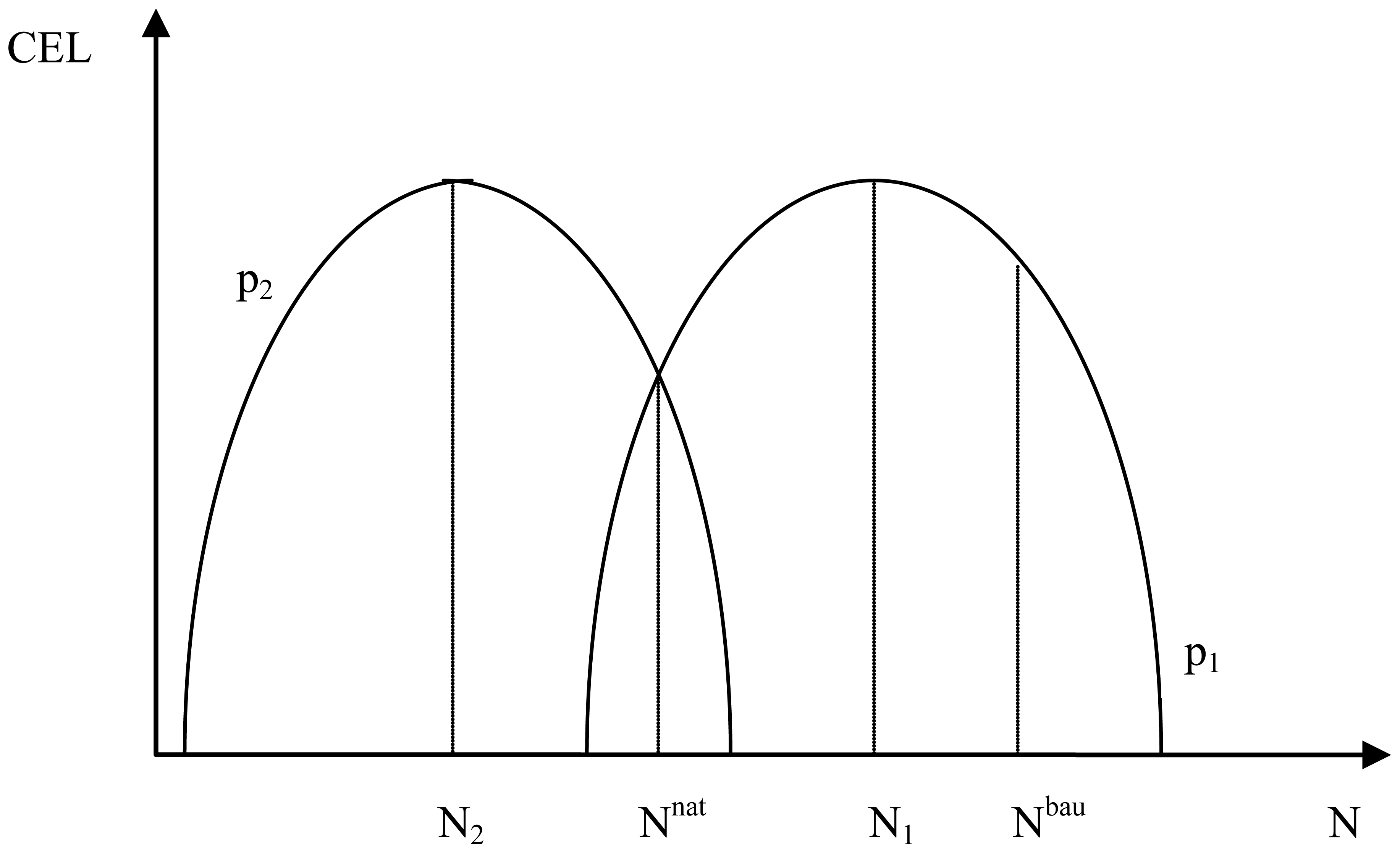
While the standard bioeconomic model would establish crab populations as a function of N levels, GEEM allows a far more detailed picture of how the levels work their way from the phytoplankton to the crabs. Beginning with the phytoplankton, their optimization problems and steady-state conditions yield parabolic relationships between N and the steady-state CEL for both dinoflagellates and diatoms [42]. The curves in Figure 2 show all the values of deep channel CEL and N for which a representative individual of diatoms (p₂) and dinoflagellates (p₁) earns zero net energy and its species' population is, therefore, in steady state. Points below (above) the curves imply low (high) CELs and positive (negative) net energies, and populations increase (decrease) until the CEL is driven up (down) to the curve. For a fixed N, the species with the highest curve would drive out its competitor species over time, because it can tolerate a higher CEL. However, with stochastic N flows, the species can coexist because they randomly take turns having the higher curve, with the dinoflagellate (diatom) populations increasing (decreasing) at higher (lower) flows.

The ideal N levels for dinoflagellates and diatoms, labelled N₁ and N₂, are where their variable respirations are lowest (see Equation (2.13)) and their parabolas at a maximum. If stochastic N levels were concentrated in a narrow range, diatoms would dominate at flows around N₂ and dinoflagellates would dominate at flows around N₁. Deviations of N from these ideal levels increases each phytoplankton's respiration for a given size; therefore, to maintain zero net energy CEL must be lower to offset the N stress. N^nat is the N level that allows the highest probability of coexistence for the two species. Elevated N flows such as those experienced over the 80's and 90's have a mean of 30% over N^nat [76], indicated in Figure 2 by N^bau. These elevated flows are termed here “business as usual” (BAU). A 100 year sequence of BAU is employed as the baseline to evaluate the consequences of N reductions.

The BAU N loads generate ecosystem externalities that can be understood using the linked general equilibrium models. Agriculture runoff causes changes in blue crab populations. These changes are a result of complex ecosystem interactions from phytoplankton, through other species, to blue crabs, as the ecosystem passes through different general equilibriums. Briefly, under BAU, the elevated N flows above N^nat lead to a phytoplankton community dominated by dinoflagellates in the deep channel. In turn this increases SOD, which causes DO in the deep channel to fall, with physiological impacts on deep channel clams, croakers and blue crabs. But, with the increased dinoflagellates, deep channel zooplankton also increase. Following diatoms, clams preying on diatoms decline substantially (and they are physiologically stressed by the lack of DO). Jellyfish mirror their zooplankton prey and increase. For mobile crab and croaker predators, both species migrate to the non-hypoxic shallows and in total their populations decline. Further, with the decline in clams and expansion of zooplankton in the deep channel, croaker substitute, or switch in ecological terminology, to a diet of more zooplankton. The effects of physiological and prey stresses in the deep channel are compounded by intense intra-species competition in the shallows, leading to the crab and croaker population declines.

The ecosystem externalities are experienced in the economy when total crab populations and harvests fall, while crab prices rise. Harvesters also switch to fishing the crab abundant shallows more intensely, with longer seasons and larger harvests in the shallows. Longer seasons in the fishery and higher fishery prices cause factors of production to flow into the fishery (although to catch fewer crabs). These factors are released by composite goods and agriculture, but as the fishery is laborintensive regional wages rise (slightly) and the regional rental rate of capital falls (slightly). Output of both sectors declines, but while agricultural prices fall as agriculture is highly capital intensive, composite prices rise given the sector's factor proportions and the higher relative increase in the wage.

5.2. Reduction in N from N^bau

To examine in detail how the ecosystem externality unfolds, the consequences of reducing N loading are investigated for a policy where the elevated levels are reduced from N^bau to N^nat in Figure 2. The reduction is initiated in period one, and then economic and ecological variables are tracked over 100 years. The changes in ecosystem variables that generate the ecosystem externalities stem from changes in predator-prey relationships, competitive advantages, physiological stresses, switching behaviors, functional responses and migration patterns, all of which are absent in the standard bioeconomic model.

Ecological Consequences

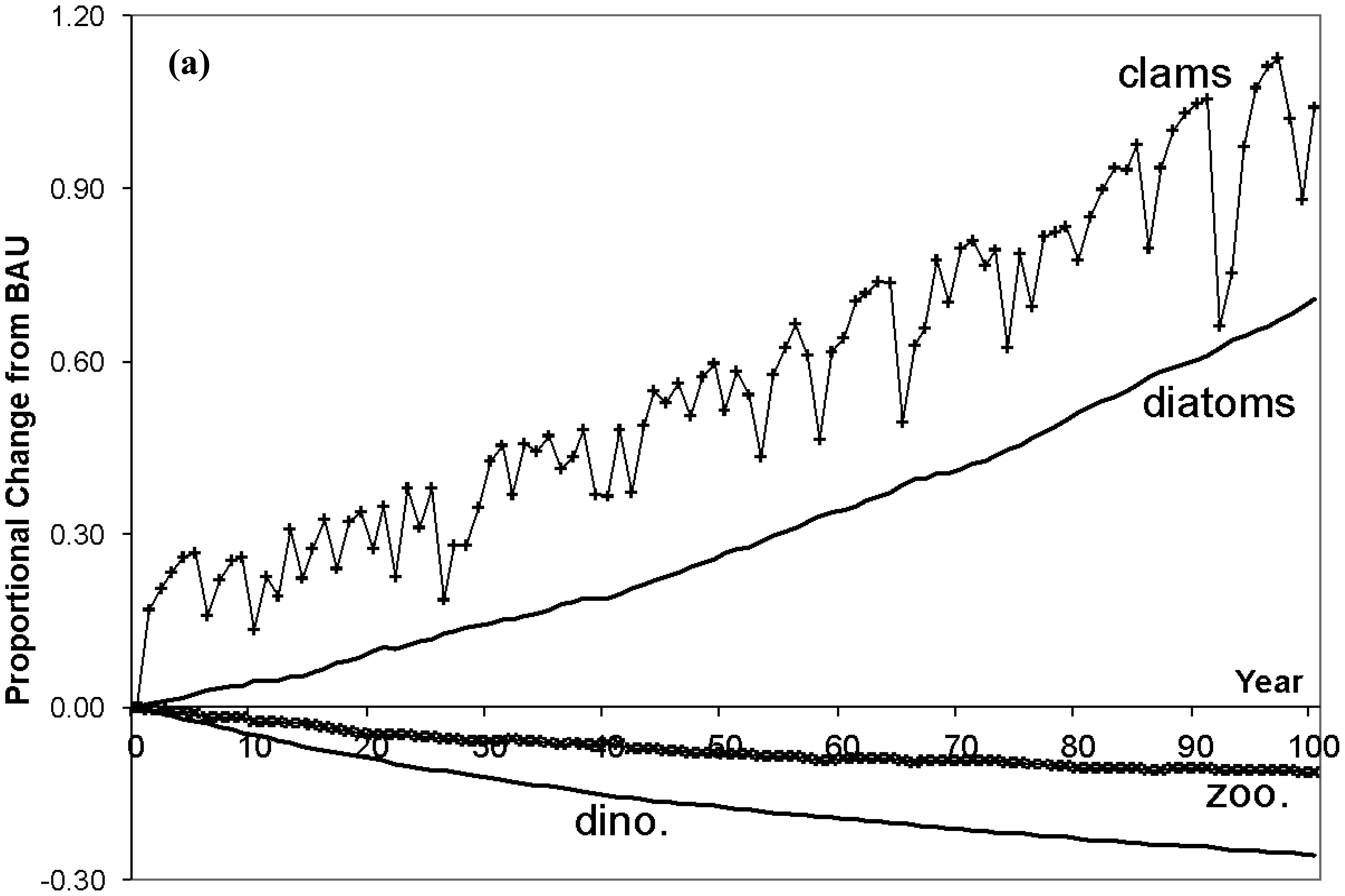
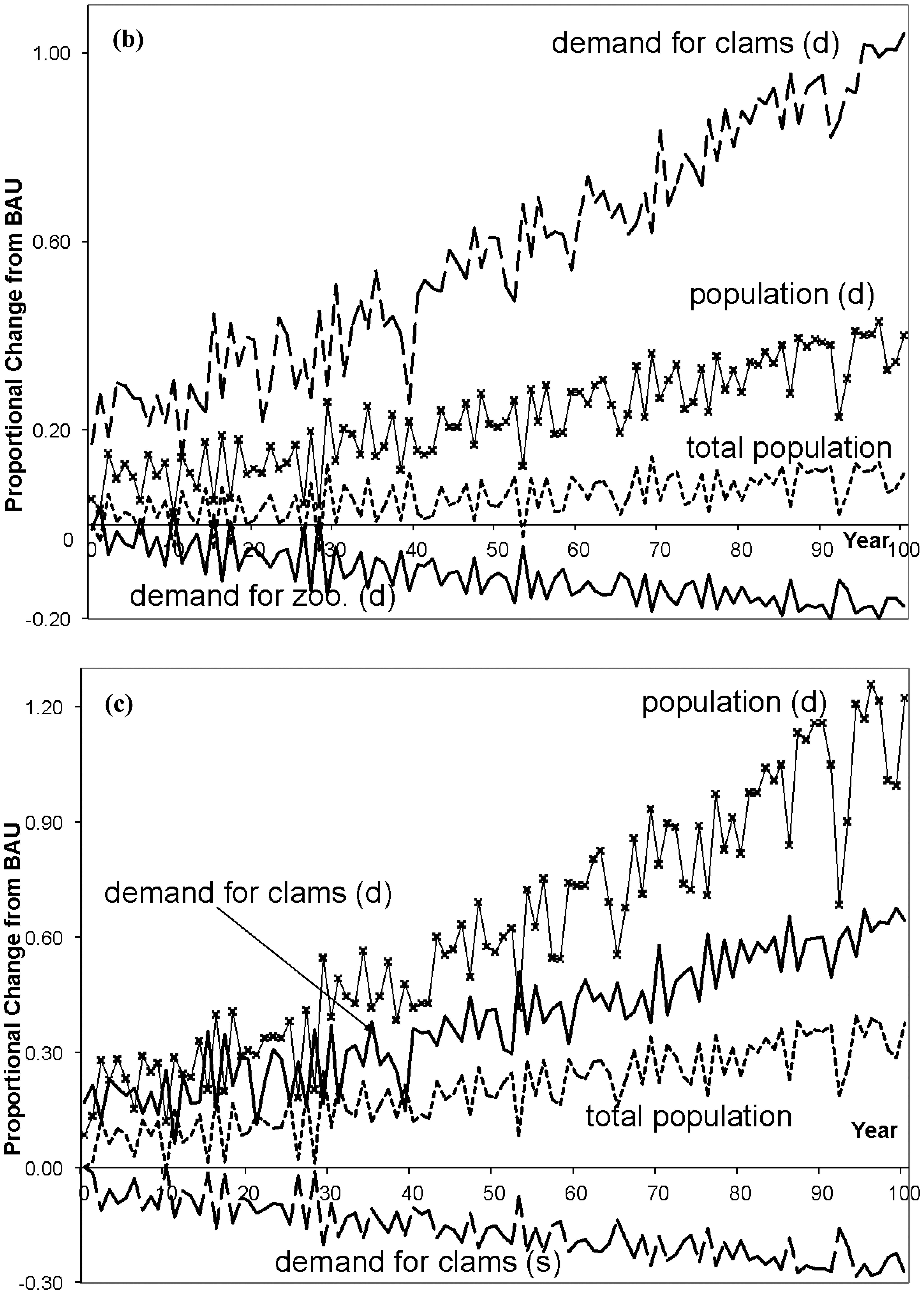
The trend lines in Figure 3 display proportional changes from BAU for selected ecosystem variables over 100 years, and

Table 3. Average seasonal percentage changes in ecosystem variables.

Scenario			No Increase in Agriculture Costs	1% Increase in Agriculture Costs	10% Increase in Agriculture Costs
Variable	Variable Type	Species	% Change From BAU	% Change From BAU	% Change From BAU
nd1	Deep populations	Dinoflagellates	−20.0800%	−20.0800%	−20.0800%
nd2		Diatoms	51.0257%	51.0257%	51.0257%
nd3		Zooplankton	−8.8283%	−8.8283%	−8.8283%
nd4,		Clams	82.2926%	82.2926%	82.2926%
nd5		Jellyfish	−6.9873%	−6.9873%	−6.9873%
n6	Populations (deep) (shallow)	Croaker	8.0706%	8.0706%	8.0706%
(nd6)			(30.1607%)	(30.1607%)	(30.1607%)
(ns6)			(−7.1604%)	(−7.1604%)	(−7.1604%)
n7,			27.4328%	27.4329%	27.4331%
(nd7,)		Blue crab	(91.3994%)	(91.3994%)	(91.3998%)
(ns7)			(−2.5262%)	(−2.5262%)	(−2.5260%)
xd63	Deep demands	Croaker for zoo.	−13.8000%	−13.8000%	−13.8000%
xd64		Croaker for clams	79.8497%	79.8497%	79.8497%
xd74		Blue crab for clams	51.5951%	51.5951%	51.5948%
ed63	Deep prices	Croaker for zoo.	28.3814%	4.0046%	28.3814%
ed64		Croaker for clams	9.7637%	6.1443%	9.7637%
ed74		Blue crab for clams	7.2958%	9.0322%	7.2959%
xs63	Shallow demands	Croaker for zoo.	−7.1934%	−7.1934%	−7.1934%
xs64		Croaker for clams	−7.1934%	−7.1934%	−7.1934%
xs74		Blue crab for clams	−20.5412%	−20.5412%	−20.5414%
es63	Shallow prices	Croaker for zoo.	4.0046%	4.0046%	4.0046%
es64		Croaker for clams	6.1443%	6.1443%	6.1443%
es74		Blue crab for clams	9.0322%	9.0322%	9.0324%

contains the average annual percentage changes in immobile deep channel and mobile species populations (shallow population changes are small and omitted from the table). The erratic patterns in the lines are due to the random N levels. First, inspect the consequences for immobile populations in the deep channel (top figure). As N loading is reduced diatoms are able to outcompete dinoflagellates for exposure to light, causing a substantial decrease in dinoflagellate biomass. In turn this reduces SOD, which causes DO in the deep channel to climb, with beneficial physiological impacts on clams, croakers and blue crabs. But, with the rapid rise of diatoms and decline of dinoflagellates, the zooplankton population falls. While there is an increase in one of zooplankton's prey populations (diatoms), this benefit is more than offset by both the decrease in their other prey (dinoflagellates), and by the rapid increase in clams (under less stress from O₂ depletion) that compete with zooplankton for diatoms. Following diatom populations, clams increase substantially as they prey only on diatoms and they are released from the physiological stress under BAU. Jellyfish (omitted from Figure 2) mirror their zooplankton prey population and decline.

Moving up the web to mobile predators, total blue crab populations rise fairly sharply (bottom Figure 3). Feeding on clams only, and given the rapid recovery of clams in the deep channel, blue crabs switch from shallow to deep clams by migrating. The migration results in a declining proportion of crabs in the shallow channel and increasing proportion in the deep channel. With the emigration from the shallows, crabs face less intra-species competition in the shallows where their population falls slightly to allow a net increase in their total population.

Given the economic underpinnings of GEEM, these population changes also can be explained in demand/price terms. Clam populations rise, increasing prey for blue crabs in the deep channel. With more abundant prey, ceteris paribus, the energy price blue crabs pay for clams would fall and each crab's demand would rise. Instead both price and demand rise. Demand rises because: (1) blue crabs are less stressed by the lack of DO, and for each unit of clam consumed a crab's respiration cost is lower making clams more attractive; and (2) the crab population increases which increases total demand. Thus the upward pressure on price from the net increase in demand by each blue crab along with the increased blue crab population, both creating more intra species competition, more than offsets the downward pressure on price from the increased clam prey. These demand/price changes mean higher optimum net energies for each crab that must precede any population increase.

Total croaker population rises over time but less dramatically than does the crab population (middle Figure 3). Croaker switching behavior is somewhat more involved than the crab's behavior as croaker have two prey species in both regions. With the reduction in N, deep channel clams recover while zooplankton decline. The prices croaker pay for both deep channel prey rise with more intense intra-specific competition, as there is rapid croaker immigration from the shallows following the reduction in respiration costs in the deep channel. The increased price for deep zooplankton leads to a fall in each croaker's demand for zooplankton. But the increased price for deep clams leads to an increase in each croaker's demand for clams. This is because the deep zooplankton price rises by relatively more than the deep clam price, such that croaker in the deep channel switch to a diet of fewer zooplankton.

While there is no change in N loading in the shallow channel by assumption, there are indirect effects due to the top predator population movements and changes. Population changes are small, but with the predator emigrations shallow zooplankton and clam populations actually decline due to the eventual increase in both top predator total populations. Simultaneously, the decrease in zooplankton and clams lowers predation pressure on diatoms and dinoflagellates. But, as clams decline by slightly more than zooplankton, the pressure on diatoms is reduced by a greater extent. This provides an advantage to diatoms in the competition for space, leading to a decline in dinoflagellates and a rise in diatoms in the shallows.

Economic Consequences

As opposed to standard fishery models, the general equilibrium framework shows how the fishery sector interacts with other sectors in the economy, and thereby provides a more complete understanding of the role renewable resources play in economic activity. The economic consequences depend crucially on how the N reductions impacts agricultural costs. Three cost scenarios are simulated: 0%, 1%, and 10% cost increases due to N reduction.

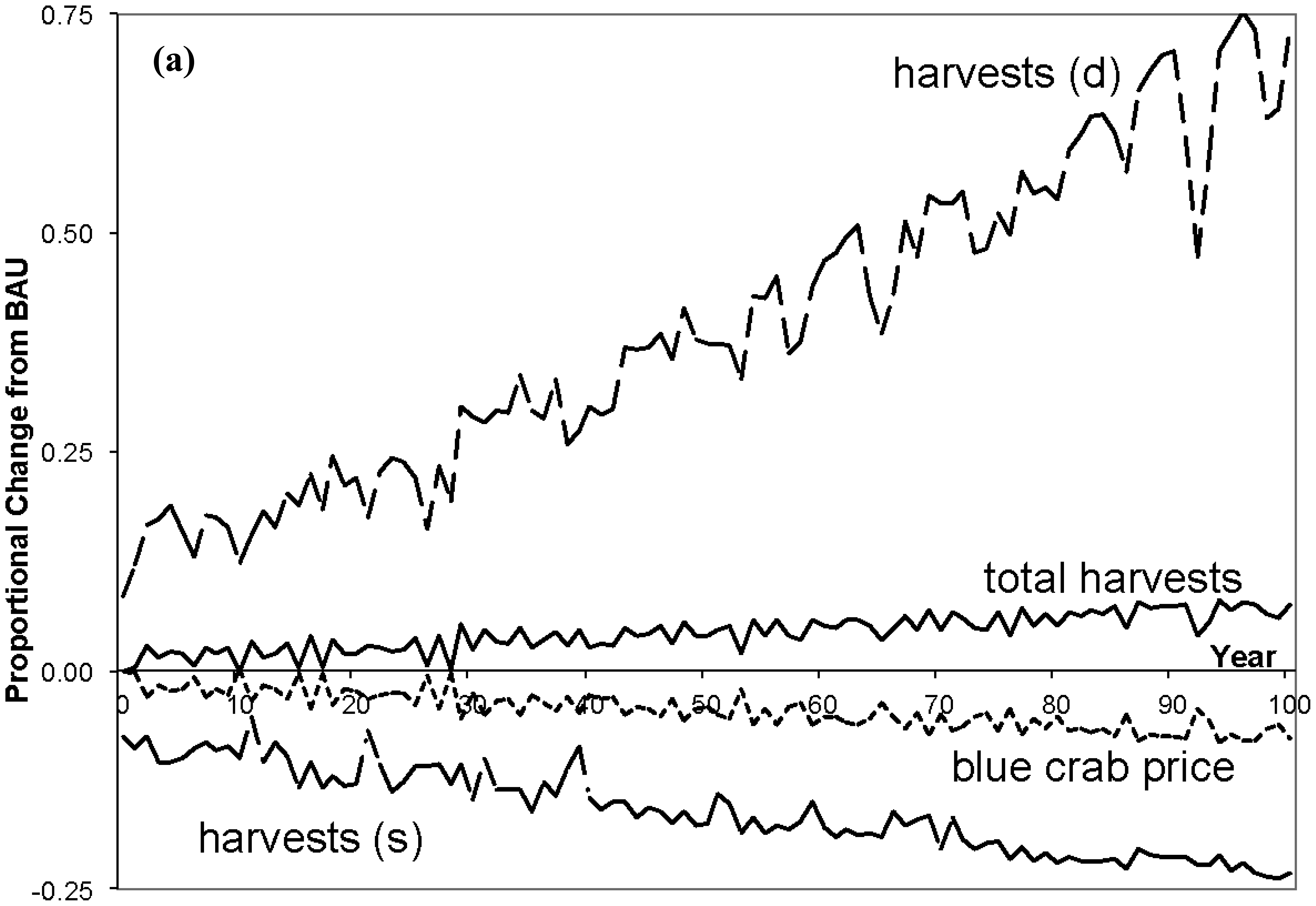
The third column in

Table 4. Average seasonal percentage changes in economic variables.

Scenario		No Increase in Agriculture Costs	1% Increase in Agriculture Costs	10% Increase in Agriculture Costs
Variable	Variable Type	% Change From BAU	% Change From BAU	% Change From BAU
I	Income	3.194E–6%	3.754E–5%	3.336E–4%
R	Capital price	6.137E–6%	7.213E–5%	6.409E–4%
PC	Composite price	3.193E–6%	3.753E–5%	3.335E–4%
PA	Agriculture price	4.155E–6%	1.0000%	10.0005%
PB	Crab price	−5.8380%	−5.8381%	−5.8381%
QC	Composite output	5.354E–6%	−0.0001%	−0.0009%
QA	Agriculture output	4.489E–6%	−0.8916%	−8.2212%
H	Crab harvest	5.6373%	5.6372%	5.6367%
(Hdeep)	(Deep)	56.5770%	56.5768%	56.5793%
(Hshallow)	(Shallow)	−18.6235%	−18.6235%	−18.6275%
T	Crab season	−0.6034%	−0.6035%	−0.6042%
(Tdeep)	(Deep)	46.6725%	46.6723%	46.6756%
(Tshallow)	(Shallow)	−23.2483%	−23.2483%	−23.2535%
KB	Crab capital	−0.6034%	−0.6035%	−0.6046%
LB	Crab labor	−0.6034%	−0.6035%	−0.6040%

presents average annual percentage changes in economic variables for the 0% case, and Figure 4 shows proportional changes over time for some of the variables. As loading is reduced, the direct impacts to the economy are largely on blue crab variables (neglecting any values associated with juvenile croaker). As total crab populations rise over time (see Figure 3), the total season length falls as there are more crabs, total harvests increase, and the prices for crabs fall. But as deep crab populations rise and shallow fall, harvesters switch from intensely fishing the shallows to a more even balance of effort over both channels, with the deep season length and harvests rising.

With larger crab populations fishery factors are more productive and require shorter seasons to harvest more crabs. The lower crab prices cause factors of production to be released from the fishery. These factors are reemployed in composite goods and agriculture (the percentage changes are very small and omitted from the table), but as the fishery is labor intensive there is a relative shortage of capital (labor is the numeraire) so that the regional rental rate of capital rises slightly. Regional incomes therefore rise. With no agricultural costs incurred by N reduction, as factor employment in agriculture increases so does its output, which is accompanied by a rise in price as agriculture is highly capital intensive. A similar response is observed in composite goods. Composite output rises along with factor employment, and its price slightly rises because of the close equality in composite factor proportions and the increase in the price of capital. Overall, output rises in each sector, prices fall for blue crab harvests, while they rise for composite and agricultural goods. Standard bioeconomic models would only capture rising harvests, and ignore all price, income, and quantity changes of other goods.

Table 5. Cumulative welfare measures for each policy and scenario from BAU.

Agricultural Cost Scenario	Cumulative Welfare (Million $) Discount Rate
	0	0.03
0	10.88	2.42
1%	−241.07	−78.90
10%	−2412.70	−779.81

presents discounted cumulative equivalent variations across each agriculture cost scenario over a 100 year time horizon, for both zero and 3% discount rates. In the absence of any agriculture cost impacts the N reductions yield a welfare improvement over BAU, with discounted welfare gains of $2.42 million. Increasing the agricultural costs from 0 to 1% finds a discounted welfare loss of $79 million, that rises to $780 million with 10% cost increase (at a discount rate of 3%).

Most of the welfare decline, when agricultural cost changes are positive, is concentrated in the agriculture sector which is much larger than the blue crab fishery. Nevertheless, there are small impacts on all ecological and economic variables that are revealed in the general equilibrium framework. As the agricultural costs are increased, agricultural prices rise by similar amounts (Table 4, columns four and five). This in turn causes agricultural demand and output to decline. But, withincreases in costs, each unit of agricultural production requires more capital and labor, leading to increased factor employment in the sector (by 0.1% for 1% agriculture cost and by 1% for 10% agricultural costs, omitted from the table). Factor price changes simultaneously cause composite goods to release factors, bringing a decline in composite output.

Impacts on blue crab harvests are more involved given the direct linkage to randomly fluctuating N flows. As agricultural costs rise, so does output price. While households reduce their agricultural consumption, their substitution is not perfect and they have to reduce both their blue crab and composite consumption. The reduction in crab demand reduces factor employment in the sector and released factors flow to agriculture. Thus the increase in harvests declines, allowing a slight increase in the blue crab population. But as the numeraire (labor) is relatively cheaper and the sector is labor intensive, the blue crab price actually falls in relation to the price spike in agricultural goods (although there are smaller harvests). With larger blue crab populations factors in the fishery become even more productive, which further shortens the fishing season and lowers fishery factor demands.

5.3. Policy Breakeven Croaker Valuations

One unique feature of incorporating multiple species is that multiple ecosystem services can be examined. Namely the blue crab harvests are directly consumed, but croaker are consumed in the future at a different stage of their life-cycle. While croaker harvests are not included in the model (although a component of future work), some inference of how they may change welfare estimates is possible.

We pose the question: “if N reductions lower welfare, what must an additional Neuse croaker recruited after N reductions be worth for reductions to be welfare neutral?” The question is pertinent for the two scenarios with positive increases in agricultural costs. We take the absolute value of each annual welfare change under increased agricultural costs (equivalent variation and losses in these cases) and divide it by that period's additional croaker (in relation to BAU). This gives the value that the additional croaker must provide for the N reductions to be welfare neutral.

Table 6. N policy breakeven Neuse croaker valuation.

Agricultural Cost Scenario	Annual Average Required Value ($) per Neuse Croaker
0	N/A
1%	0.46
10%	4.54

presents the annual average of these calculations over the three agricultural cost scenarios, for the 100 year horizon. If agricultural costs are assumed to increase by 1%, then on average each Neuse croaker must be worth at least 46 cents. This value increases to $4.54 if agricultural costs are increased by 10%.

The magnitudes depend on critical assumptions in the economic and ecological components of the model. Further, these inferred valuations are over juvenile croaker who may never survive to adulthood. But using data from [77] the average wholesale price per pound of Atlantic croaker between 1994 and 2000 was $0.35 (2002 dollars). Further, using data on recreational landings for Atlantic coast states [78] the average weight of a croaker was 0.91 pounds, yielding a price per average croaker of $0.32. Thus if it is assumed that each additional Neuse croaker reaches maturity and can be caught, then under the 1% increase in agricultural costs, the N reduction policy appears worthwhile (assuming constant croaker prices over time) if the retail markup for croaker is at least 44% (enough to raise the $0.32 to $0.46). For the 0% increase in agricultural costs, N reduction is worthwhile, and for the 10% increase the reduction is unlikely to be worthwhile.

6. Discussion

Although ecosystems provide myriad services to economies, only one service is considered in most economic renewable resource models. The more complete bioeconomic model introduced here makes clear that economic policies and activities influence myriad services. We demonstrate that N reduction in the Neuse has consequences throughout the ecosystem and economy owing to the joint determination of important variables. The reduction altered levels of all ecosystem populations, economic factor reallocation, changes in all regional prices, incomes, demands, outputs and both ecological welfare (in terms of species populations) and economic welfare (in terms of equivalent variations).

Inserting ecological detail into economic models is a promising new approach that raises numerous research issues. We will briefly discuss three issues that fall out of our linked Neuse models. First, the models reveal linked economic inefficiencies that suggest coordination in correcting the inefficiencies may be important. Agricultural runoff into the Neuse is a negative externality imposed on the blue crab industry, and the lack of property rights for blue crabs creates familiar open access harvesting problems. Finding an optimum level of runoff requires knowing its damage costs, and these will depend on the property rights regime in the fishery. Introducing mechanisms such as a transferable runoff permit system into agriculture and an individual transferable quota system in the fishery would work to establish property rights over the two externalities. To establish an efficient outcome requires linking the systems as any change in either property right has indirect consequences on the other.

The second issue that falls out of the analysis is how boundaries of the systems are defined. Whether to use partial or general equilibrium analysis is a common question in economics that carries over to ecosystems. In the Neuse the economics could be confined to the crab fishery, or broadened to include other estuary fisheries, or further to include agriculture, to include North Carolina, the Southeast region, and so on. Similarly, the ecosystem could be confined to crabs, or to include crabs and their prey in the estuary, to their competitor croakers in the estuary, to the croakers adult stage in the ocean and ocean going species, and so on. Regardless of where the boundaries are drawn around the systems there are going to be leakages to and from outside the systems, and this requires judicious selection of those variables that will significantly impact the results but not unduly complicate the model.

Thirdly, the linked approach incorporates the economic value of “non-economic” species. The linkages between most species and humans are not direct, but they are indirect through ecosystem services and food web linkages. The systems approach of the ecological and economic systems accounts for these indirect linkages by providing some interpretation of welfare changes owing to changes in non-economic species populations. For example, zooplankton are not directly linked to humans, but in the ecosystem they are an intermediate good in that they are prey for jellyfish and croakers. Since croakers have direct economic value to humans, a positive imputed value can be assigned to zooplankton. At the same time, overabundant jellyfish can hamper recreational activities such as swimming and boating implying that there may be a negative imputed value to zooplankton. Further, the disaggregated nature of the modeling approach provides a foundation easily adaptable to incorporate numerous other linkages through production processes and the specification of utility functions.

In sum, the CGE/GEEM linked modeling approach is flexible and can be applied to numerous other conflicts that arise when economic development and environmental conservation appear at odds. Three links between the Neuse economy and ecosystem were explored, but others could be added to the analysis. For example, including the croaker populations and their ecosystem outside the estuary would expand the economic model to include commercial and recreational croaker harvests. Additionally, existence values or other use values such as birding in the estuary are presumably significant (evidenced in the vast research dedicated towards the Neuse estuary), and incorporating them could result in different welfare impacts.

References and Notes

- Bradford [2] provides an illuminating example on the incidence of a tax.
- Bradford, D.F. Factor prices may be constant but factor returns are not. Econ. Lett. 1978, 1, 199–203. [Google Scholar]
- See [4] or [5] for supportive arguments and [6] for a summary.
- Arrow, K.; Daily, G.; Dasgupta, P.; Levin, S.; Maler, K.-G.; Maskin, E.; Starrett, D.; Sterner, T.; Tietenberg, T. Managing ecosystem resources. Environ. Sci. Technol. 2000, 34, 1401–1406. [Google Scholar]
- Bockstael, N.E.; Freeman, A.M., III; Kopp, R.J.; Portney, P.T.; Smith, V.K. On measuring economic values for nature. Environ. Sci. Technol. 2000, 34, 1384–1389. [Google Scholar]
- Tschirhart, J. Integrated ecological-economic models. Ann. Rev. Resour. Econ. 2009, 1, 381–409. [Google Scholar]
- Crocker, T.D.; Tschirhart, J. Ecosystems, externalities and economies. Environ. Resour. Econ. 1992, 2, 551–567. [Google Scholar]
- Strong, A.; Finnoff, D.; Tschirhart, J. Is economic growth for the birds? Ecol. Econ. 2011, 70, 1375–1380. [Google Scholar]
- In a series of papers Eichner and Pethig also link general equilibrium economic and ecological systems and like GEEM they ground the ecological system in individual optimization. [10] and [11] are examples.
- Eichner, T.; Pethig, R. Ecosystem and economy: An integrated dynamic general equilibrium approach. J. Econ. 2005, 85, 213–249. [Google Scholar]
- Eichner, T.; Pethig, R. Pricing the ecosystem and taxing ecosystem services: A general equilibrium approach. J. Econ. Theory 2009, 144, 1589–1616. [Google Scholar]
- Stephens, D.W.; Krebs, J.R. Foraging Theory; Princeton University Press: Princeton, NJ, USA, 1986. [Google Scholar]
- Gurney, W.S.C.; Nisbet, R.M. Ecological Dynamics; Oxford University Press: New York, NY, USA, 1998. [Google Scholar]
- Quirk, J.P.; Smith, V.L. Dynamic economic models of fishing. In H.R. MacMillan Lectures in Fisheries, Economics of Fisheries Management: A Symposium; Scott, A.D., Ed.; Institute of Animal Resource Ecology, University of British Columbia: Vancouver, Canada, 1970. [Google Scholar]
- Clark, C.W. Mathematical Bioeconomics: The Optimal Management of Renewable Resources, 2nd ed.; Wiley: New York, NY, USA, 1990. [Google Scholar]
- Hannesson, R. Optimal harvesting of ecologically interdependent fish species. J. Environ. Econ. Manag. 1983, 10, 329–345. [Google Scholar]
- Conrad, J.M.; Adu-Asamoah, R. Single and multispecies systems: The program of tuna in the Eastern Tropical Atlantic. J. Environ. Econ. Manag. 1986, 13, 50–68. [Google Scholar]
- Flaaten, O. Bioeconomics of sustainable harvest of competing species. J. Environ. Econ. Manag. 1991, 20, 163–180. [Google Scholar]
- Conrad, J.M.; Salas, R. Economic strategies for coevolution: Timber and butterflies in Mexico. Land Econ. 1993, 69, 404–415. [Google Scholar]
- Flaaten, O.; Stollery, K. The economic costs of biological predation. Environ. Resour. Econ. 1996, 8, 75–95. [Google Scholar]
- Stroebele, W.J.; Wacker, H. The economics of harvesting predator-prey systems. J. Econ. 1995, 61, 65–81. [Google Scholar]
- Wacker, H. Optimal harvesting of mutualistic ecological systems. Resour. Energy Econ. 1999, 21, 89–102. [Google Scholar]
- Baird, D.; Ulanowicz, R.E. The seasonal dynamics of the chesapeake bay ecosystem. Ecol. Monogr. 1989, 59, 329–364. [Google Scholar]
- Christensen, V.; Pauly, D. ECOPATH II—A software for balancing steady-state ecosystem models and calculating network characteristics. Ecol. Model. 1992, 6, 169–185. [Google Scholar]
- MRAG Americas Inc. A Review of Approaches To Fisheries Management Based on Ecosystem Considerations, with Particular Emphasis on Species Interactions; Alaska Fisheries Science Center: Seattle, WA, USA, 2000. [Google Scholar]
- Baird, D.; Christian, R.R.; Peterson, C.H.; Johnson, G.A. Consequences of hypoxia on estuarine food web and ecosystem function: Energy diversion from consumers to microbes. Ecol. Model. 2004, 14, 805–822. [Google Scholar]
- Christian, R.R.; Dmae, J.K.; Johnson, G.A.; Peterson, C.H.; Baird, D. Monitoring and Modeling of the Neuse River Estuary, Phase 2: Functional Assessment of Environmental Phenomena Through Network Analysis.; North Carolina State University Water Resources Research Institute Report #UNC-WRRI 2003-343-E; North Carolina State University: Raleigh, NC, USA, 2003. [Google Scholar]
- Smith, R.L. Ecology and Field Biology, 4th ed.; Harper Collins: New York, NY, USA, 1990. [Google Scholar]
- Copeland, B.J.; Tenore, K.R.; Horton, D.B. Oligohaline Regieme. In Coastal Ecosystems of the US; Odum, H.T., Copeland, B.J., McMahan, E.A., Eds.; Conservation Foundation: Washington, DC, USA, 1974; Volume 2, pp. 55–98. [Google Scholar]
- According to [31] energy is the most frequently chosen maximand in ecological maximization models, and energy per time maximization as adopted here originates with [32,33] and expanded to multiple species in [7] and to the individual level in [34]. Energy per time is also the individual's objective in the extensive optimum foraging literature, e.g., [12]. More net energy leads to larger populations. Thus the model could be interpreted as fitness maximization which is a widely accepted objective in the literature, although a fitness objective function is seldom specified.
- Herendeen, R. Do economic-like principles predict ecosystem behavior under changing resource constraints? In Theoretical Studies Ecosystems: The Network Perspective; Burns, T., Higashi, M., Eds.; Cambridge University Press: New York, NY, USA, 1991. [Google Scholar]
- Hannon, B. The structure of ecosystems. J. Theor. Biol. 1973, 41, 535–546. [Google Scholar]
- Hannon, B. Marginal product pricing in the ecosystem. J. Theor. Biol. 1976, 56, 253–267. [Google Scholar]
- Tschirhart, J. General equilibrium of an ecosystem. J. Theor. Biol. 2000, 203, 13–32. [Google Scholar]
- Lima, S.L.; Dik, L.M. Behavioral decisions made under the risk of predation: A review and prospectus. Can. J. Zool. 1990, 68, 619–640. [Google Scholar]
- A problem of interpretation arises in the maximization problem, because once an animal is successfully preyed upon, it is gone. To avoid this discrete, zero/one issue, the maximization problem is assumed to represent the ‘average’ member of the species. Thus, when the animal is captured it does not lose its entire biomass, but rather it loses biomass equal to the mean loss over all members of its species.
- Because plants ‘prey’ on the sun, their equilibrium conditions differ from (2.6). Each plant is part of a population that together with other plant populations occupies a fixed volume of water. Thus there is a limit on the amount of biomass that a water column contains. We assume the limit can be expressed in terms of water surface area, so if ni is the ith plant species population and there are p plant species, then this limit is expressed as . A is the maximum physical surface area (cm2). The phytoplankton are competing for light by building biomass, although it is space that is in limited supply and A can be thought of as the resource plants compete for.
- An unattached appendix provides more details.
- Tilman, D. Resources: A graphical-mechanistic approach to competition and predation. Am. Nat. 1980, 116, 362–393. [Google Scholar]
- Tilman, D. The resource-ratio hypothesis of plant succession. Am. Nat. 1985, 125, 827–852. [Google Scholar]
- Tilman, D. Plant Strategies and the Dynamics and Structure of Plant Communities; Princeton University Press: Princeton, NJ, USA, 1988. [Google Scholar]
- Finnoff, D.; Tschirhart, J. Identifying, preventing and controlling successful invasive plant species using their physiological traits. Ecol. Econ. 2005, 52, 397–416. [Google Scholar]
- Pacala, S.W.; Tilman, D. Limiting similarity in mechanistic and spatial models of plant competition in heterogeneous environments. Am. Nat. 1994, 143, 222–257. [Google Scholar]
- Tilman, D.; Polasky, S.; Lehman, C. Diversity, productivity and temporal stability in the economies of humans and nature. J. Environ. Econ. Manag. 2005, 49, 405–426. [Google Scholar]
- Asner, G.P.; Wessman, C.A. Scaling PAR absorption from the leaf to landscape level in spatially heterogeneous ecosystems. Ecol. Model. 1997, 103, 81–97. [Google Scholar]
- Tschirhart, J. Resource competition among plants: From optimizing individuals to community structure. Ecol. Model. 2002, 148, 191–212. [Google Scholar]
- Norberg, J.; Swaney, D.P.; Dushoff, J.; Lin, J.; Casagrandi, R.; Levin, S.A. Phenotypic diversity and ecosystem functioning in changing environments: A theoretical framework. Proc. Natl. Acad. Sci. 2001, 98, 11376–11381. [Google Scholar]
- We are indebted to conversations and helpful references provided by Marty Smith in developing this component of the model.
- Smith, M.D.; Crowder, L.B. Valuing ecosystem services with fishery rents: A lumped-parameter approach to hypoxia in the neuse river estuary. Sustainability.
- Borsuk, M.E.; Stow, C.A.; Higdon, D.; Reckhow, K.H. A Bayesian hierarchical model to predict benthic oxygen demand from organic matter loading in estuaries and coastal zones. Ecol. Model. 2001, 143, 165–181. [Google Scholar]
- Borsuk et al. [50 provide a functional form for where L is carbon loadings (herein taken to be nuisance phytoplankton biomass), h is depth, and a, b, and k are parameters. From this . The value calculated employed Borsuk's parameter estimates and average Neuse loadings and depth.
- Borsuk, M.E.; Powers, S.P.; Peterson, C.H. A survival-based model of the effects of bottom-water hypoxia on the density of an estuarine clam (Macoma balthica). Can. J. Fish. Aquat. Sci. 2002, 59, 1266–1274. [Google Scholar]
- The elasticity estimate was found by linear regression of log-transformed data. The adjusted R2 = 0.954 demonstrates a reasonable measure of fit, and while the slope coefficient's standard error of 0.116 is significant at the 10% level of significance the intercept was not significantly different than zero.
- Mistiaen, J.A.; Strand, I.E.; Lipton, D. Effects of environmental stress on blue crab (Callenectes sapidus) harvests in Chesapeake bay tributaries. Estuaries 2003, 26, 316–323. [Google Scholar]
- Shoven, J.B.; Whalley, J. Applying General Equilibrium; Cambridge University Press: Cambridge, UK, 1992. [Google Scholar]
- Ballard, C.L.; Fullerton, D.; Shoven, J.B.; Whalley, J. A General Equilibrium Model for Tax Policy Evaluation; The University of Chicago Press: Chicago, IL, USA, 1985. [Google Scholar]
- De Melo, J.; Tarr, D. A General Equilibrium Analysis of US Foreign Trade Policy; MIT Press: Cambridge, MA, USA, 1992. [Google Scholar]
- Finnoff, D.; Tschirhart, J. Linking dynamic economic and ecological general equilibrium models. Resour. Energy Econ. 2008, 30, 91–114. [Google Scholar]
- An exception is [60] who present an analysis that deliberately separates fixed and variable inputs in a partial equilibrium model of a fishery regulated through TAC's and a limited entry program.
- Weninger, Q.; McConnell, K.E. Buyback programs in commercial fisheries: Efficiency versus transfers. Can. J. Econ. 2000, 33, 394–412. [Google Scholar]
- Defined as the difference between initial expenditure and that expenditure necessary to achieve the post-policy level of satisfaction at initial prices.
- Finnoff, D.; Tschirhart, J. Protecting an endangered species while harvesting its prey in a general equilibrium ecosystem model. Land Econ. 2003, 79, 160–180. [Google Scholar]
- Given a focus on relative changes, a unitless measure of annual N flows is employed, with an arbitrary value of 2 in the benchmark. BAU is a 30% increase in this to 2.6. As N flows are assumed to be normally distributed, for each a standard deviation of 0.3 is employed in all simulations.
- Eggleston, D.B.; Johnson, E.G. Population Dynamics and Stock Assessment of the Blue Crab in North Carolina; Final Report for Contracts 99-FEG-10 and 00-FEG-11 to the North Carolina Fishery Resource Grant Program; North Carolina Sea Grant, and the North Carolina Department of Environmental Health and Natural Resources, Division of Marine Fisheries: Raleigh, NC, USA, 2004. [Google Scholar]
- Petipa, T.S.; Pavlova, E.V.; Mironov, G.N. The food web structure, utilization and transport of energy by trophic levels in the planktonic communitities. In Marine Food Chains; Steele, J.H., Ed.; Oliver & Boyd: Edinburgh, UK, 1970. [Google Scholar]
- Hall, R.O. Department of Zoology; University of Wyoming: Laramie, WY, USA, Personal communication.
- Puget Sound Information. King County: Washington, DC, USA, 2011. Available online: http://www.kingcounty.gov/environment/waterandland/puget-sound-marine/beaches/carkeek.aspx (accessed 20 September).
- Estes, J.A.; Duggins, D. O. Sea otters and kelp forests in Alaska: Generality and variation in a community ecological paradigm. Ecol. Monogr. 1995, 65, 75–100. [Google Scholar]
- Eby, L.A.; Crowder, L.B.; McClellan, C.M.; Peterson, C.H.; Powers, M.J. Impacts of habitat degradation from intermittent hypoxic disturbances on demersal estuarine fishes. Working paper. In Nicholas School of the Environment and Earth Sciences; Duke University: Marine Lab, Durham, NC, USA, 2004. [Google Scholar]
- Selberg, C.D.; Eby, L.A.; Crowder, L.B. Hypoxia in the Neuse River estuary: Responses of blue crabs and crabbers. North Am. J. Fish. Manag. 2001, 21, 358–366. [Google Scholar]
- NASA. The Dead Zone. The Earth Observatory: Washington, DC, U.S.A., 2011. Available online: http://earthobservatory.nasa.gov/Features/FloydFear/fear_3.php (accessed September 20).
- Jensen, T.C.; Verschoor, A.M. Effects of food quality on life history of the rotifer Brachionus calyciflorus Pallas. Freshw. Biol. 2004, 49, 1138–1151. [Google Scholar]
- Hill, K. Mercenaria Mercenaria. Smithsonian Marine Station at Fort Pierce: Fort Pierce, FL, USA. Available online: http://www.sms.si.edu/irlspec/mercen_mercen.htm (accessed 20 September 2011).
- Dineen, J. Vallentinia Gabriellae. Smithsonian Marine Station at Fort Pierce: Fort Pierce, FL, USA. Available online: http://www.sms.si.edu/irlspec/vallen_gabrie.htm (accessed 20 September 2011).
- Stow, C.A.; Borsuk, M.E.; Stanley, D.W. Long-term changes in watershed nutrient inputs and riverine exports in the Neuse River, North Carolina. Water Res. 2001, 35, 1489–1499. [Google Scholar]
- Paerl, H.; Pinckney, J.; Fear, J.; Peierls, B. Ecosystem responses to internal and watershed organic matter loading: Consequences for hypoxia in the eutrophying Neuse River Estuary, North Carolina, USA. Mar. Ecol. Prog. Ser. 1998, 166, 17–25. [Google Scholar]
- Burgess, C.C.; Bianchi, A.J. An Economic Profile Analysis of the Commercial Fishing Industry of North Carolina Including Profiles for State-Managed Species; NOAA Award No. NA16FW1543; North Carolina Department of Environment and Natural Resources: Morehead City, NC, USA, 2004. [Google Scholar]
- 2001 Review of the Fishery Management Plan for Atlantic Croaker (Micropogonias undulatus). Atlantic States Marine Fisheries Commission: Arlington, VA, USA, 2001. Available online: http://www.asmfc.org/ (accessed on 15 September).
© 2011 by the authors; licensee MDPI, Basel, Switzerland. This article is an open access article distributed under the terms and conditions of the Creative Commons Attribution license (http://creativecommons.org/licenses/by/3.0/).
Share and Cite
Finnoff, D.; Tschirhart, J. Inserting Ecological Detail into Economic Analysis: Agricultural Nutrient Loading of an Estuary Fishery. Sustainability 2011, 3, 1688-1722. https://doi.org/10.3390/su3101688
Finnoff D, Tschirhart J. Inserting Ecological Detail into Economic Analysis: Agricultural Nutrient Loading of an Estuary Fishery. Sustainability. 2011; 3(10):1688-1722. https://doi.org/10.3390/su3101688
Chicago/Turabian StyleFinnoff, David, and John Tschirhart. 2011. "Inserting Ecological Detail into Economic Analysis: Agricultural Nutrient Loading of an Estuary Fishery" Sustainability 3, no. 10: 1688-1722. https://doi.org/10.3390/su3101688