Groundwater Potential Mapping Using Data Mining Models of Big Data Analysis in Goyang-si, South Korea

Abstract

Recently, data mining analysis techniques have been developed, as large spatial datasets have accumulated in various fields. Such a data-driven analysis is necessary in areas of high uncertainty and complexity, such as estimating groundwater potential. Therefore, in this study, data mining of various spatial datasets, including those based on remote sensing data, was applied to estimate groundwater potential. For the sustainable development of groundwater resources, a plan for the systematic management of groundwater resources should be established based on a quantitative understanding of the development potential. The purpose of this study was to map and analyze the groundwater potential of Goyang-si in Gyeonggi-do province, South Korea and to evaluate the sensitivity of each factor by applying data mining models for big data analysis. A total of 876 surveyed groundwater pumping capacity data were used, 50% of which were randomly classified into training and test datasets to analyze groundwater potential. A total of 13 factors extracted from satellite-based topographical, land cover, soil, forest, geological, hydrogeological, and survey-based precipitation data were used. The frequency ratio (FR) and boosted classification tree (BCT) models were used to analyze the relationships between the groundwater pumping capacity and related factors. Groundwater potential maps were constructed and validated with the receiver operating characteristic (ROC) curve, with accuracy rates of 68.31% and 69.39% for the FR and BCT models, respectively. A sensitivity analysis for both models was performed to assess the influence of each factor. The results of this study are expected to be useful for establishing an effective groundwater management plan in the future.

1. Introduction

In recent years, spatial data collected from remote sensing platforms have accumulated in various fields, and the use of large spatial datasets has spread widely. As data is created and managed in a variety of ways, it becomes increasingly important to analyze the complexity of the data and to understand the relationships within the data. Complex and uncertain data objects require analysis; for such a data-driven analysis, data mining techniques have been developed that can enhance the usability of big data and could be applied in various fields [1,2]. Groundwater potential is one of the most difficult fields for estimation, as it is impossible to conduct direct measurements in all areas; the groundwater potential is the potential of an area to be an aquifer that could be used for groundwater development. Therefore, in this study, we analyzed the relationships between the groundwater potential and the remote sensing data based on various spatial data related to groundwater.

For an efficient groundwater quality management, areas with a high amount of developable groundwater resources should be investigated first. The accurate estimation and prediction of groundwater production characteristics are necessary for the efficient utilization and systematic management of groundwater resources. To obtain exact measurements, conventional exploration methods used for various groundwater-related factors must be considered, along with their complex interactions. This method requires considerable time, money, and manpower for field research. Additionally, the presence of groundwater in a particular area depends on factors catalogued in big data: topography, geological structures, lithology, fracture density, connectivity, slope, groundwater potential, and changes in these factors based on climatic conditions. Therefore, recently developed big data methods, particularly data mining models, should be applied to the analysis of groundwater potential. The regional groundwater potential could be easily assessed using data mining models prior to field-based hydrogeological resistivity surveys to simplify the interpretation of the relationships between the hydrogeological factors and the groundwater pumping capacity.

With regards to water management, water security is essential to actively deal with environmental threats due to economic changes or natural disasters [3]. In particular, changes in environmental conditions such as increased drought due to climate change, industrialization, urbanization, nuclear power plant accidents, and other disasters have underscored the importance of ensuring sustainable and high-quality water resources. Groundwater resources with high levels of safety against environmental threats are considered a key future resource [4]. To effectively preserve and manage groundwater resources in preparation for expected social and natural environmental changes, the developable amount of groundwater must first be evaluated.

Korea uses around 3.7 billion tons of groundwater per year, accounting for about 10% of its total water use, which is 35% of the developable amount of groundwater [5]; 50% is from the river water, and 40% is from the dam facility of the remaining 90% of the source. Developable groundwater, which is the groundwater development potential, refers to the amount of groundwater that can be pumped from the aquifer continuously within a range that does not destroy the water circulation system and does not cause groundwater disturbances [6]. Changes in the land use and demand for groundwater in response to industrialization and urbanization have led to regional biases in groundwater resources [7]. As a result of pollution caused by natural and anthropogenic pollutants due to industrial development and land use changes, the interest in maintaining and preserving high-quality groundwater in sufficient quantities has increased. The effects of climate change, such as drought, floods, and sea level rise, affect the supply of water underground [8]. Groundwater is not an infinite source of water, and once it is polluted, considerable amounts of time and money are required to clean and restore it. It is necessary to establish a plan for the efficient use and management of groundwater resources through an exploration of their current status and usage [9].

The increasing demand for water along with the expected changes in aquatic environments due to global climate change highlight the urgent need for a quantitative methodology that can represent groundwater production. A groundwater potential model based on changes in temperature and rainfall patterns was developed that evaluates the vulnerability of groundwater [10]. In addition, studies on the sustainability of domestic groundwater resources [11] and changes in agricultural water availability due to climate change [12] have been carried out at the regional level. However, due to the uncertainty and complexity of groundwater potential, a groundwater productivity assessment methodology has not yet been established. It is difficult for local government officials or policymakers to determine groundwater management priorities. Thus, the sustainable and efficient management of groundwater resources based on a data-driven analysis of groundwater potential is essential.

Numerous studies have used geographic information system (GIS) analysis methods to map the groundwater potential with thematic layers such as topography, soils, lithology, and drainage patterns [13,14,15,16]. Aquifer potential maps have been developed in New Zealand, a country with a very similar hydrogeological and meteorological landscapes to Korea [17]. Several countries have attempted to develop an aquifer potential map, but they are complex and require large efforts. Therefore, the data mining model is an effective way to estimate the groundwater potential.

Probabilistic models have also been applied to groundwater potential mapping using a multi-criteria decision analysis and weights-of-evidence modeling [18,19]. The weights of different factors were measured and assigned based on personal judgment and local information [20]. Other assessments using machine-learning models such as decision trees, fuzzy logic, and numerical modeling which provided more sophisticated results [21,22,23]. To derive additional thematic layers, the integration of remote sensing and geophysical surveys with GIS has been attempted [15,24,25]. A study based on remote sensing data was also conducted for groundwater potential mapping [9,15,25,26]. However, previous studies have been limited to the GIS analysis of groundwater potential rather than big data methods. Spatial correlations could be derived when a number of interspersed spatial layers indicate a relationship with a specific event such as the groundwater pumping capacity. In terms of being able to analyze basic statistical trends of the big data, the frequency ratio (FR) models were applied in various study areas [27,28,29,30]. Also, the FR model has been applied to assess the groundwater potential [18,19,31]. The FR model is a simple statistic method to analyze the correlation between the groundwater-related factors and groundwater potential. Additional data mining models such as the boosted classification tree (BCT) model and GIS-based approaches have not yet been used to describe the groundwater potential. The boosted tree model is one of the big data analysis techniques applied to various fields in recent years [32,33,34,35]. After the selection of the groundwater-related factors by FR model, a data mining model of BCT model could derive the additional quantitative analysis of the relationships between the groundwater-related factors and groundwater potential.

The purpose of this study was to map and analyze the groundwater potential in Goyang-si, South Korea using the FR and BCT data mining models. The satellite-based thematic layers such as topography, land cover, soil, and forest and the geological, hydrogeological, and precipitation characteristics were analyzed. Thematic maps generated from remote sensing data as source data were used; aerial photographs and satellite images including Kompsat-2 and Kompsat-3 were used to derive the topographical, land use, soil, forest, and geological maps used in this study. Using spatial analysis techniques, a correlation analysis was performed with the groundwater pumping capacity data, and the characteristics of groundwater potential were derived from the hydrogeological characteristics. Based on these results, the groundwater potential of Goyang-si was calculated and the groundwater pumping capacity data were used for comparative test. The FR model simplified the probabilistic relationships between the dependent and independent variables to quantify the relationships between the reclassified hydrological factors and groundwater capacity. The relationships calculated using the FR model enabled the easier interpretation of the groundwater potential indicated by the rating of each factor. Also, the factors used in this study are derived based on remote sensing data, and the use of remote sensing-based data could activate the application researches of remote sensing.

2. Study Area

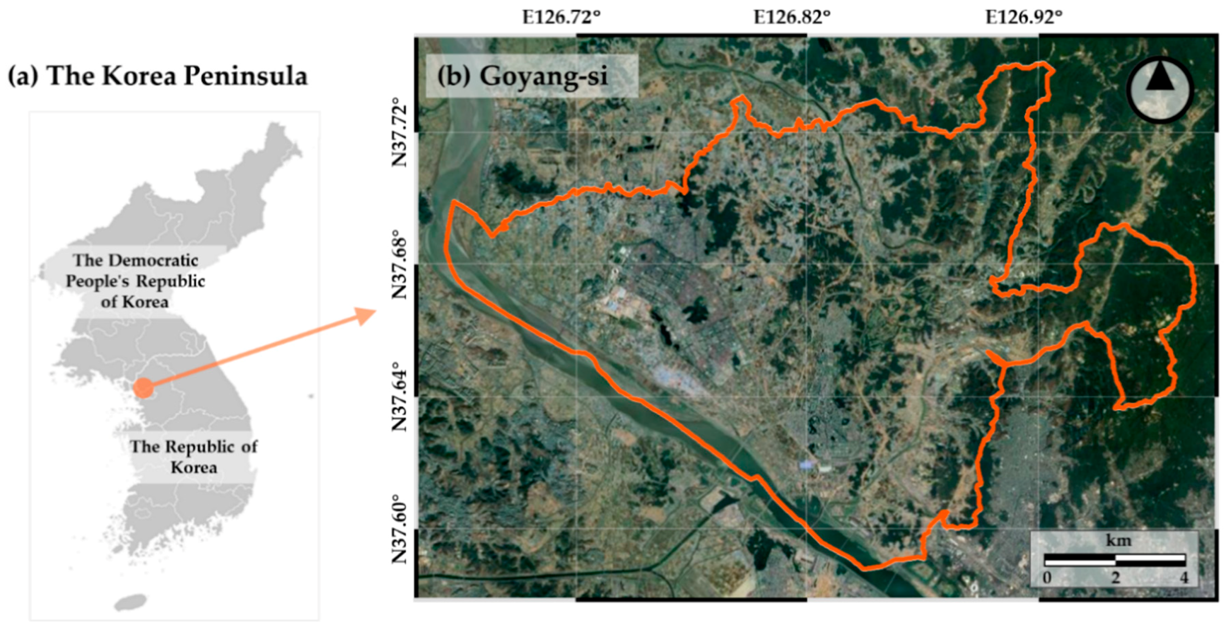
The study area is Goyang-si which is the administrative district under Gyeonggi-do near the Seoul metropolitan area (Figure 1). It is surrounded by Yangju-si to the northeast, Seoul metropolitan city to the southeast, Kimpo-si to the southwest, and the Han River and Paju-si to the north. It is located at 126°40′ E to 126°59′ E longitude, 37°34′ N to 37°44′ N latitude. Goyang-si covers an area of 267.36 km² and has a population of 102,456 as of 2015. This area experiences 350 mm of rainfall per month during the rainy season of July and August.

The geology of Goyang-si is composed of granite gneiss in the south and crystalline gneiss in the northeast. It is located in the lower Han River, and mostly consists of plains, but there is a steep mountainous area in the eastern portion with a high average elevation, which is a branch of the Gwangju mountain range, with the main mountain of Bukhansan (836 m). Thus, the study region is composed of high mountainous areas in the east and lowland hills and riverbed sediments in the west. The northeastern part of the study area contains low hills with mountainous forests in the middle area and relatively large sedimentary plains in the west along the Han River and Gokrung stream. This area includes diverse land uses, with urban and agricultural areas. However, currently, most of the study area is city area, and there is little water imported from the outside for agricultural purposes. The water supply system mainly services urban areas, whereas the outer city center and agricultural areas use a considerable amount of groundwater for household and agricultural purposes. The system supplies agricultural water through many wells and does not draw water from the outside of the city.

More than 9000 underground water exploitation facilities exist in Goyang-si. The rate of ground water use of the city is approximately 1007.49 m³ per year, indicating that groundwater resources have been actively developed and utilized [36]. The total amount of water resources in Goyang-si was 343,266 × 10³ m³ per year, of which 82,832 × 10³ m³ per year or 24.13% was lost due to evapotranspiration and 260.443 × 10³ m³ per year or 75.87% was outflow. Based on an analysis of the total outflow as the direct outflow, intermediate outflow, and base outflow, 176,811 × 10³ m³ per year, corresponding to 51.51% of the total water resources, was discharged directly or through intermediate leaching. The basin runoff corresponding to the amount of groundwater potential was calculated as 83,637 × 103 m³ per year, which is 24.36% of the total water resources. The groundwater potential depends on the distribution and reliability of the pumping capacity data as well as the changes in the factors evaluated or the addition of pumping capacity data [37]. Therefore, it is necessary to evaluate the groundwater potential to support the sustainable use of groundwater in the study area and to prepare groundwater management measures based on the quantitative results of this evaluation.

3. Spatial Datasets

To create a map of the groundwater potential in Goyang-si, a spatial database of the groundwater data and related influencing factors was constructed. Various remote sensing-based data including topographic, land cover, and forest maps were collected and utilized for data mining. Each dataset is derived from aerial photographs and satellite images, and these datasets are independently managed by various agencies. In this study, we created a spatial database integrating numerous data types provided by the governmental institutions.

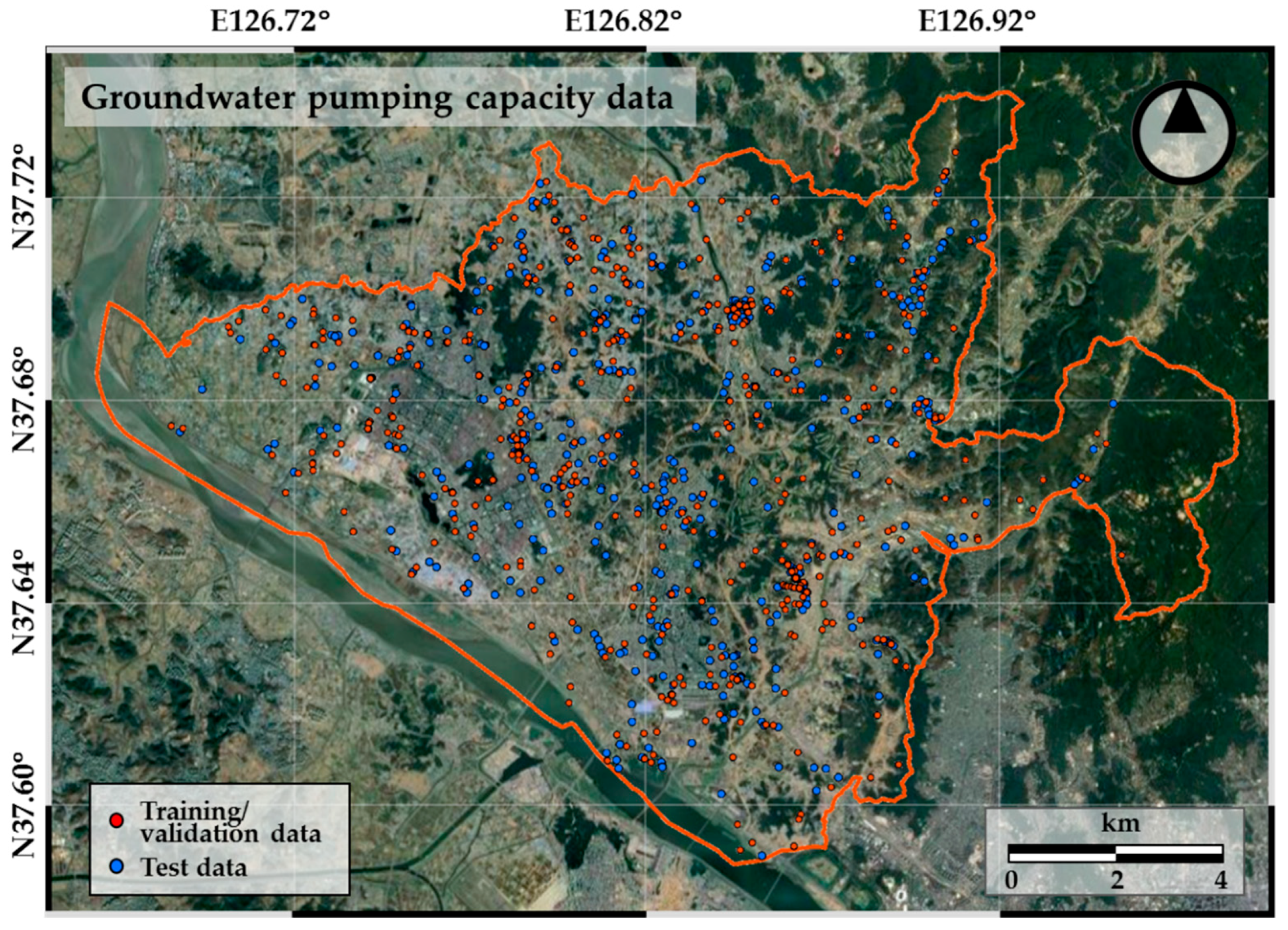
Groundwater pumping capacity data were collected, and a groundwater location map was generated from the basic groundwater survey report based on field observations of the Korea Rural Community Corporation (Figure 2). This data was acquired during 2006–2009 as a result of the pumping test, which is a test for observing changes in the head of aquifers in aquifers during a certain period of time. Approximately 8700 pumping test data of groundwater were assembled from the field observations, and among them, a total of 876 pumping capacity data were selected, accounting for the top 10% of total pumping capacity data. The selected data were then randomly classified into a training dataset of 438 (50%) aquifers, while the remaining 438 (50%) were used for test [33,38,39,40,41]. A total of 13 groundwater-related influencing factors were selected; these factors were extracted and calculated from satellite-based data including topographic, land cover, soil, forest, and hydrological maps, as well as Automatic Weather System (AWS) data obtained from the government and other organizations.

A pumping test is a field experiment to determine the permeability coefficient and the storage coefficient of an aquifer by interpreting the water-level response obtained from one or more observation wells. The hydrogeological map was produced for this study area; the hydraulic conductivity and storage coefficient were obtained based on the hydrogeological map from the basic groundwater survey report that was published by the Korea Rural community Corporation [6].

Table 1. The groundwater characteristics by hydrogeological unit [6].

Category	Division	Paragneiss	Unconsolidated Sediment
Permeability coefficient	Number of wells	50	6
	Maximum	32.69	770.50
	Minimum	0.04	4.43
	Mean	4.31	176.20
	Median	1.54	38.80
	Standard Deviation	8.05	299.95
Storage coefficient	Number of wells	41	-
	Maximum	0.2250	-
	Minimum	0.0004	-
	Mean	0.0420	-
	Median	0.0216	-
	Standard Deviation	0.0546	-

summarizes the permeability coefficient and storage coefficient of each hydrogeological map.

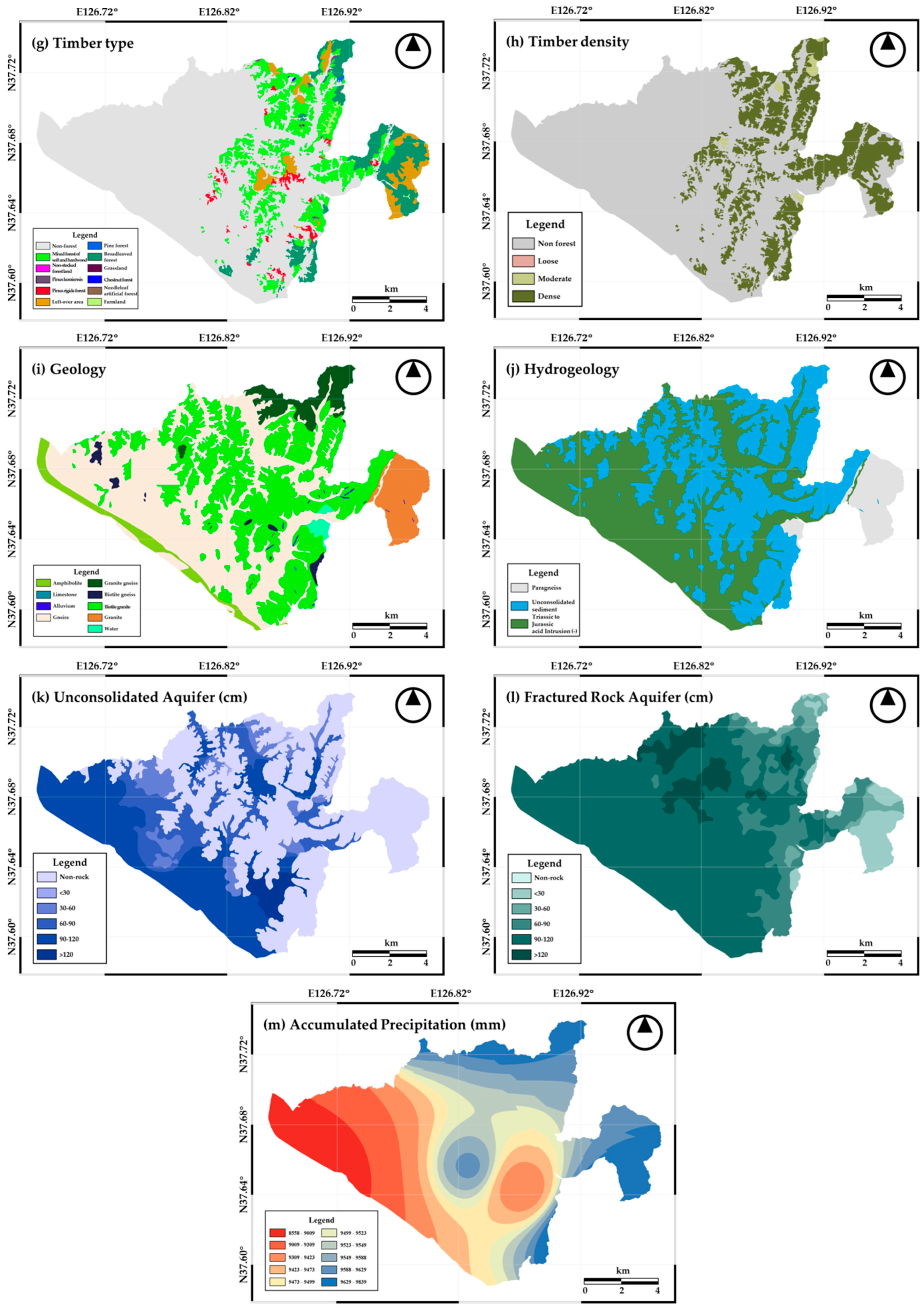
Various thematic maps derived from remote sensing data as source data were used in this study (

Table 2. The data layers describing the groundwater potential within the study region.

Category	Factors	Data Type	Scale (Year)	Source Data
Underground water pumping capacity data a	Training Test	Point	-	Field survey
Topographic map b	DEM (m) Slope (°)	GRID	1:5000 (2006–2016)	Aerial photograph
Land cover map c	Land Cover	Polygon	1:5000 (2012)	Aerial photograph, Kompsat-2 and -3
Soil map d	Soil Drainage Soil Texture Soil Depth	Polygon	1:5000 (1998~2006)	Aerial photograph, Field survey
Forest map e	Timber type Timber density	Polygon	1:25,000 (2004–2006)	Aerial photograph, Field survey
Geological map f	Geology	Polygon	1:50,000 (2004)	Aerial photograph, Field survey
Hydrogeological map g	Hydrogeology Unconsolidated Aquifer Fractured Rock Aquifer	Polygon	1:50,000 (2009)	Field survey
Precipitation h	Accumulated Precipitation	Point	-	AWS

^a The training and test data from the basic groundwater survey report from field observations by the Korea Rural Community Corporation. ^b The topographical factors were extracted from a digital topographic map by the National Geographic Information Institute (NGII; http://www.ngii.go.kr). ^c The land cover map released by the Ministry of Environment of Korea. ^d The detailed soil map produced by the Rural Development Administration (RDA; http://www.rda.go.kr). ^e The forest map produced by the Korea Forest Service (KFS; http://www.forest.go.kr). ^f The geological map produced by the Korea Institute of Geoscience and Mineral Resources (KIGAM; http://www.kigam.re.kr). ^g The hydrogeological map produced by K-water (K-water; www.kwater.or.kr). ^h The accumulated precipitation of 2008–2014 from 14 Automatic Weather System (AWS) observatories.

). For the topographical map, the geographical data is acquired by numerical mapping using an analytical plotter from the aerial photographs taken from 2006; additional corrections were performed and updated by a field survey with the enlarged image for the areas not readable in aerial photographs. For the land use map, aerial photographs with 0.25 m of spatial resolution taken in 2012 were classified into 22 medium classification level categories by using an automatic image classification method. In addition, the classification accuracy was evaluated, and the quality was examined by using Kompsat-2 with 1 m of spatial resolution and Kompsat-3 with 0.7 m of spatial resolution of spatial resolution image data and digital topographical map. Soil maps are produced by conducting field surveys based on the basic map which is made by interpreting aerial photographs using stereoscopic images, such as the color or texture. The forest map is also produced by aerial photograph interpretation and with field investigations. The geological and hydrogeological maps are generated through field surveys and office investigation focusing on the fundamental map generated from aerial photographs.

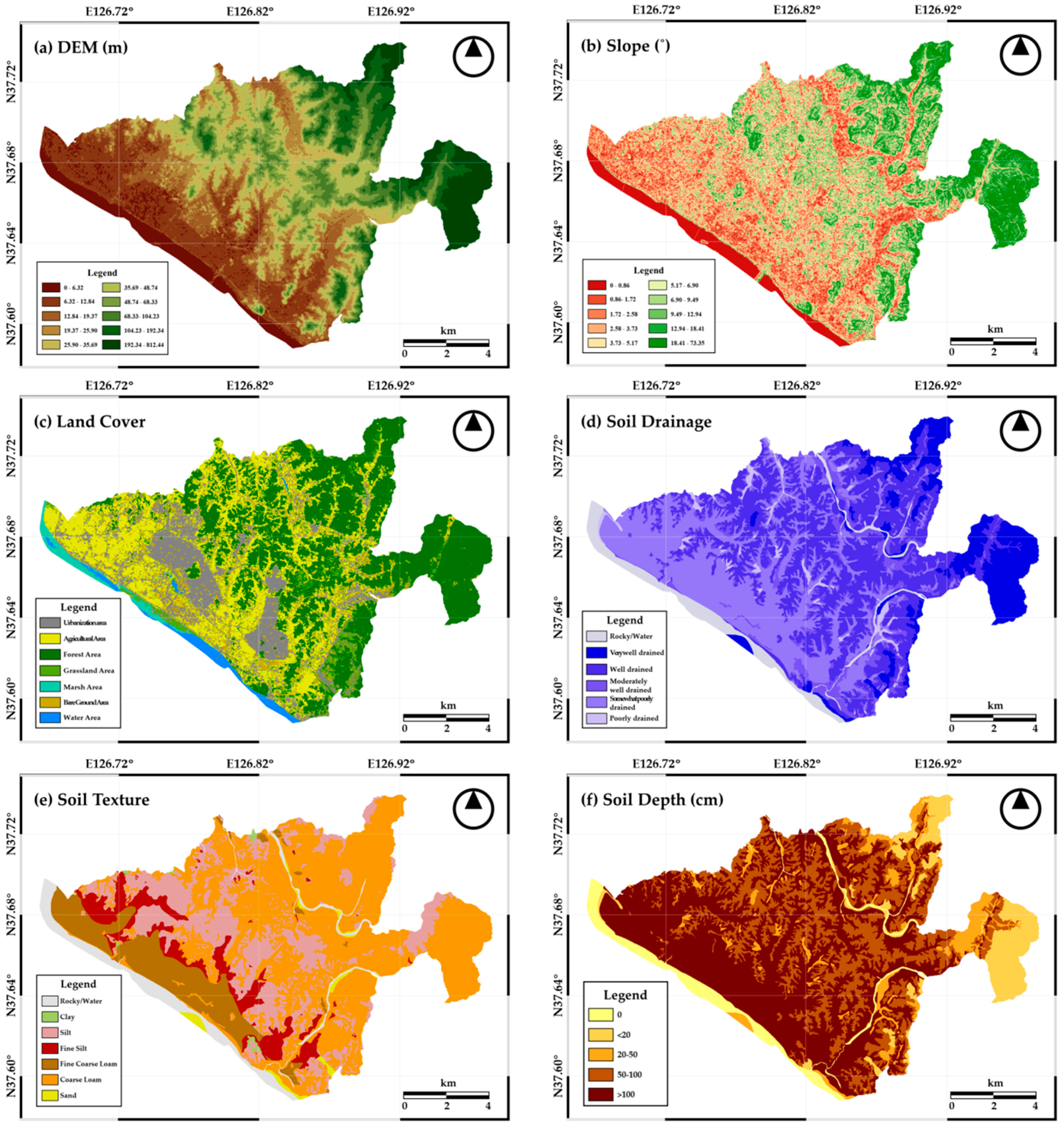
The elevation and slope of the topographical factors were extracted from the digital elevation model (DEM) using a 1:5000 digital topographic map from the National Geographic Information Institute (NGII), which was produced from aerial photographs acquired in 2015. Topography is affected by erosion and sedimentation; thus, it is an important factor influencing many physical and chemical environmental variables because it affects the composition and migration of groundwater, soil, and surface water [42]. The land cover data were extracted from the 1:50,000 land cover map issued by the Ministry of Environment. The land cover maps were generated from aerial photographs with Kompsat-2 and -3 satellite images and classified into 22 medium classification level categories. Due to the size of the study area, it is difficult to show the medium level of classification categories so that it is reclassified into seven categories: urbanized area, agricultural area, forest area, grassland area, marsh area, bare ground area, and water area.

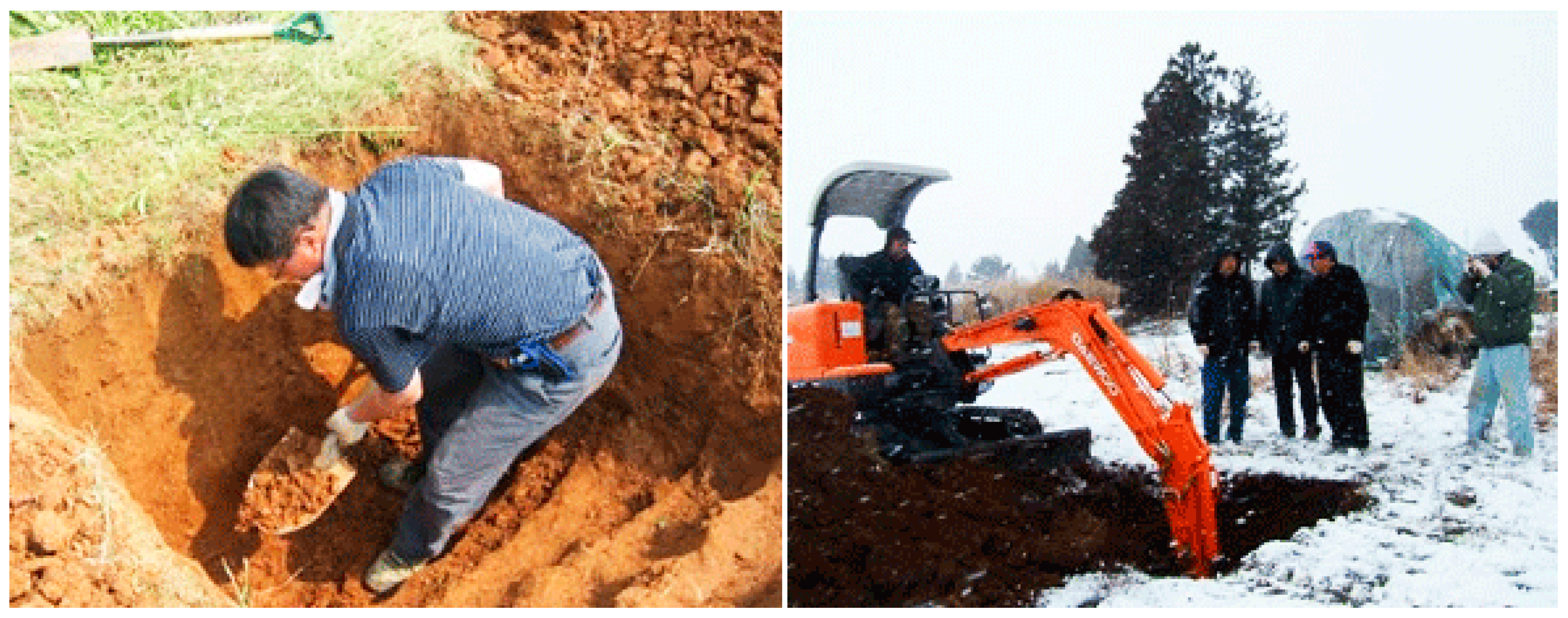
Drainage density is a factor related to permeability and surface runoff that indirectly affects the groundwater potential of the study area. The higher the density of the drainage area, the lower the permeability and the more surface runoff is produced [26]. Therefore, soil drainage, soil texture, and soil depth factors were extracted from a detailed 1:25,000 soil map issued by the Rural Development Administration (RDA). The soil data were produced by constructing cross-sectional data through digging and layering by the RDA in Figure 3. Soil drainage is divided into five grades from very well drained to poorly drained, and soil texture is divided into six classes: clay, silt, fine silt, fine coarse loam, coarse loam, and sand. Soil depth was divided into four grades ranging from very shallow (less than 20 cm) to very deep (more than 150 cm). The timber type and timber density factors were also used for this study. Timber type affects the soil moisture since the different characteristics of the roots determine the soil strength and moisture content, affecting the evapotranspiration. Also, the forest soil is affected by the timber density since the intensity of radiation and the soil moisture is related to the forest density [43]. The timber type and timber density were determined based on the 1:25,000 forest map produced by the Korea Forest Service (KFS). Based on previous digital forest mapping data generated since 1996, this map was updated and supplemented with a database of forest aerial photographs built from 2004 to 2006. Specifically, the map was modified based on the criteria of forest classification, which was confirmed through local verification if necessary.

This study considered lithology as a geological factor, which was extracted from 1:50,000 digital geological maps created in 2004 by the Korea Institute of Geoscience and Mineral Resources (KIGAM). Considering the types of lithology present, the lithology in the study area was divided into 11 groups including limestone, dyke, alluvium, and gneiss. In addition, the geologic age was considered for hydrological geology, and thus, the factors of paragneiss, unconsolidated sediment, and Triassic to Jurassic acid intrusion were extracted. Alluvial and fractured rock aquifers were also extracted from the hydrogeological map in a basic groundwater survey report that was published by the Korea Rural community Corporation [6].

The precipitation data in millimeter units were calculated from the average precipitation in 2008–2014 based on 14 AWS stations. AWS is a system to observe the weather elements such as precipitation in real time at certain areas; the precipitation data from 14 AWS stations were used in this study from the Korea Meteorological Administration and Gyeonggi-do Provincial Government: Gangseo (9450), Mapo (9645.3), Eunpyung (10,079.5), Gimpo (8499 and 9003), Goyang (9606.5 and 9869), Paju (7985.5, 10,000.5, and 9303.5), Geumgok (9712.5), Geumchon (9346), Dorasan (9746.5), and Juksung (8846). The 14-point precipitation averages for the 7 years before and after the construction of thematic maps for the spatial database were rasterized using an inverse distance weighting (IDW) interpolation.

The DEM, slope, and accumulated precipitation were reclassified into 10 classes each, and the remaining categorical factors were used as described above. The groundwater characteristics and influencing factors used in this study were constructed as a spatial database with a spatial resolution of 5 m using ArcGIS 10.3. The spatial database to which the FR and BCT models were applied is shown in Figure 4.

4. Methodology

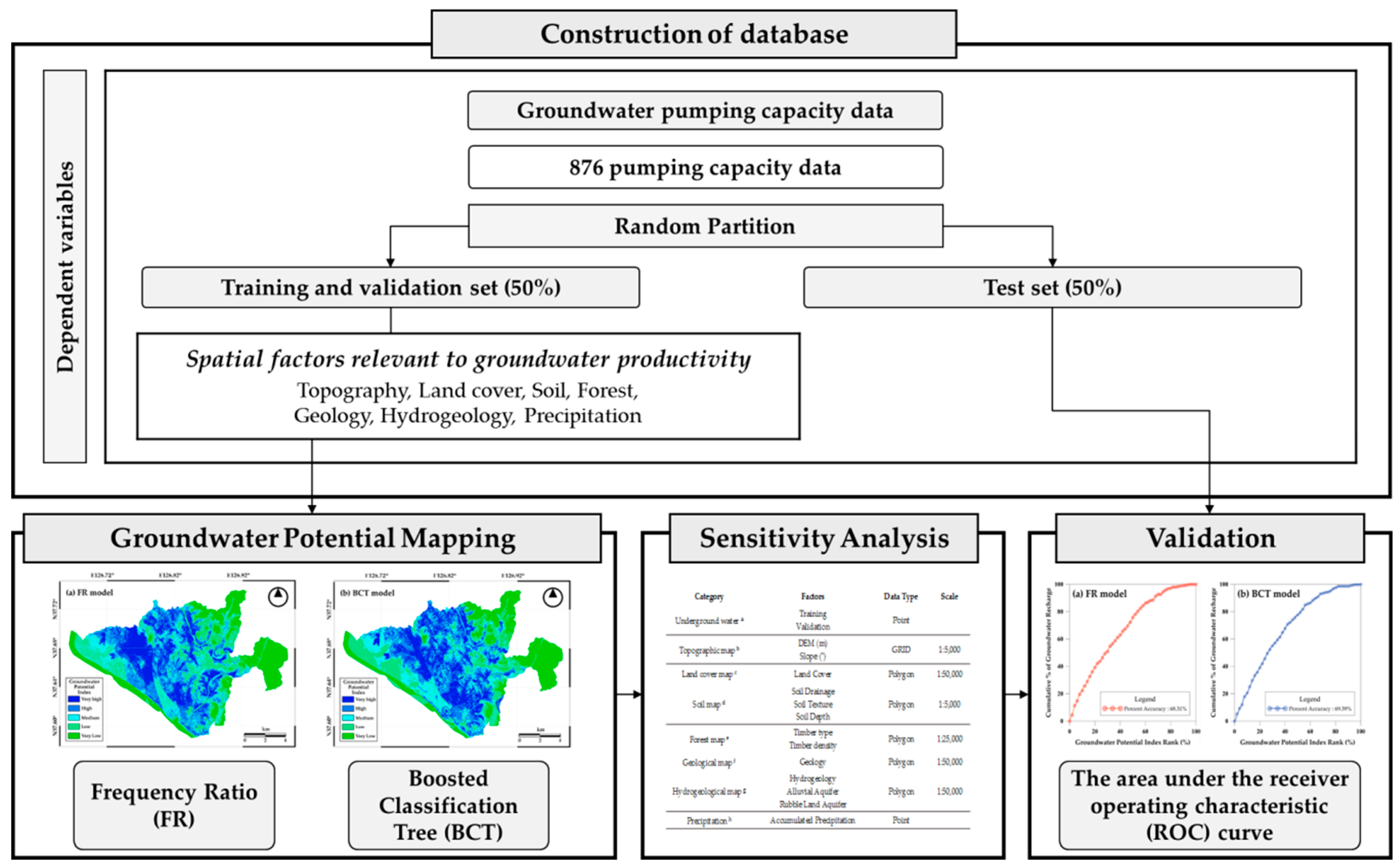
The estimation of the groundwater potential was performed using a big data analysis based on increasingly complex data related to accumulated groundwater. Specifically, among various big data analysis methodologies, the data mining techniques of FR and BCT were applied to the geospatial dataset constructed in this study; also, a sensitivity analysis was performed. The pumping test data were limited due to the economic and regional situation of the study area. Therefore, in this study, an estimation of the values in regions without data was performed through the use of a probabilistic model based on hydrogeological factors. The methodology of this study is outlined in Figure 5.

FR is a standard statistical model used for basic correlation analyses between data. The FR model was used to calculate probabilities from the groundwater pumping capacity data in each class of each factor. The BCT model is a classification tree model that uses an ensemble learning method to connect several weak classifiers and to adjust their weighting to enhance the prediction ability. The advantage of BCT is that it easily measures the relative importance of each factor. The BCT model was applied to quantify the factors of groundwater potential and their relationships with each hydrogeological factor in this study. Therefore, for the data-based analysis, the precedence correlation analysis was performed through the statistical analysis method of FR first, and the BCT was applied based on the selected groundwater related factors.

The groundwater pumping capacity data described above were used as dependent variables, whereas the groundwater-related influencing factors were considered independent variables. Groundwater pumping capacity data derived from the pumping test were gathered, and all data except the top 10% were removed. Only the values representing a pumped water quantity over 54 (m³/day) were extracted based on the upper 10% criterion so that an amount of groundwater is considered to be sufficient. To apply the data mining models FR and BCT, the top 10% of groundwater pumping capacity data were assigned a value of 1, whereas the other data were represented by 0. The groundwater pumping capacity data were randomly extracted with their statistical properties and divided into training and test datasets with 438 points, half of the well points that met the upper 10% criterion, in each dataset. For the training step, a 3-fold cross-validation methodology was used. Three random samples were generated from the training samples, and two of the three sample sets were used to model the classification tree. The remaining one sample set was used for the validation to provide accuracy for the prediction and to adjust the BCT, and this process was repeated. The models used in this study are described in detail below.

4.1. FR Model

The FR model, a bivariate statistical method, was used as a geospatial evaluation tool to determine the probabilistic relationships between dependent and explanatory variables [45]. The FR model is defined as the probability ratio of nonoccurrence to occurrence of a given element [46]. In this study, the FR model was defined as the ratio of the area where groundwater wells with an amount of water above a certain reference level were located to the total study area. The FR model was based on the correlation between the distribution of groundwater locations and groundwater-related factors and the observed relationship. To apply the FR model, groundwater-related influencing factors were classified into ten classes using the quantile classification technique. The FR values for each grade of groundwater-related influencing factors are described by Equation (1) [47].

$$FR=\frac{R_{trn}}{R_{total}},$$

(1)

where $R_{trn}$ is the ratio of the number of wells in the class of each factor to the total number of wells above the reference value and $R_{total}$ is the ratio of the number of pixels in the class of each factor to the number of pixels in the entire study area.

The FR value was calculated according to Equation (1) by dividing the ratio of each factor by the ratio of the class of the factor to the total area. An FR value of 1 represents the mean, and values higher than 1 indicate that the correlation between groundwater and groundwater-related factors is stronger than average, whereas smaller values represent lower correlations [48]. The final FR value of the groundwater potential was calculated by merging all the FR values of groundwater-related factors using the overlay function in the ArcGIS software.

4.2. BCT Model

Boosting is an ensemble learning methodology that creates strong learners through the use of multiple weak learners and is a binary response classification algorithm [49]. It combines the predictions from a set of weak classifiers, and eventually their average predictions form a strong classifier. A single-split classification tree is a weak classifier used in the AdaBoost algorithm, which forms a sequence of trees using updated data with new weighting. Each data case is classified in the current tree sequence, and the weights are determined from this classification to create the next tree. A misclassified case is assigned a higher weight than a correctly classified case, resulting in the largest weight being given to cases where classification is difficult. This process increases the probability of correct classification based on weights. The final classification step is determined by the importance of that classification across the tree sequence. AdaBoost can be examined from a statistical point of view, which clarifies the boosting process and allows it to become a function in approximation-based or additive models [50]. In addition, gradient boosting is similar to AdaBoost but with the addition of a classifier to compensate for errors. However, gradient boosting is a method used for training a new model to reduce the residual error in the pre-learning phase rather than for updating the weight of the data sample at each learning step. A boosted tree constructed using gradient boosting was found to be a very accurate predictor with a complex dataset, and therefore, the BCT model in the STATISTICA 10.3 software was applied for groundwater potential mapping.

The BCT is performed as follows. After generating a coded variable for each class with a value of 1 or 0, a different boosting tree is fitted to each category or class of categorical dependent variables to determine whether the observations show an appropriate result. The residual for the subsequent boosting step is calculated through logistic transformation. Finally, logistic transformation is applied to the prediction for each value of 1 and 0 to calculate the associated classification probability [51]. For the BCT model in STATISTICA 10.3, the learning rate was set to 0.01. The tree complexity was set to 5, and the bag fraction was set to 0.5. Given the training set, BCT calculates the prediction probability through Equation (2).

$$P\left(y=1|x\right)=\frac{1}{1+\exp (-{{\displaystyle \sum }}_{m=1}^M{h}_m\left(x\right))},$$

(2)

where $h_m\left(x\right)$ represents a single decision tree and M is the number of iterations with an input dataset of $\mathrm{Z}=\left\{\left(X_1,Y_1\right),\dots ,\left(X_n, Y_n\right)\right\}$.

$$f_0\left(x\right)=\log \frac{p_1}{1- p_1},$$

(3)

where $f_0\left(x\right)$ is the initial approximation and $p_1$ is an object in the first class used for optimal initial approximation of the sigmoid function. The gradient of L is calculated iteratively.

$$g_i= \frac{dL\left(y_i, f_m\left(x_i\right)\right)}{d f_m\left(x_i\right)},$$

(4)

where $g_i$ is the target, i.e., the groundwater pumping capacity data in this study. To calculate the maximum of Equation (4), the gradients of all objects in the dataset are calculated, moving in the direction of the gradient. A new decision tree $h_m\left(x\right)$ is created and added to the ensemble so that the composition maximizes likelihood.

5. Result

5.1. Relationships between Groundwater Potential Area and Related Factors

Table 3. The frequency ratios of the groundwater potential and related factors.

Factor	Class	No. of GP	% of GP	No. of Pixels in Domain	% of Pixels in Domain	Frequency Ratio
DEM (m)	0–6.32	6	1.37	738,934	6.93	0.2
	6.32–12.84	62	14.16	1,750,252	16.42	0.86
	12.84–19.37	73	16.67	1,268,615	11.91	1.4
	19.37–25.90	67	15.3	1,020,539	9.58	1.6
	25.90–35.69	73	16.67	1,156,821	10.86	1.54
	35.69–48.74	74	16.89	1,142,494	10.72	1.58
	48.74–68.33	44	10.05	1,052,033	9.87	1.02
	68.33–104.23	26	5.94	900,333	8.45	0.7
	104.23–192.34	12	2.74	828,311	7.77	0.35
	192.34–812.44	1	0.23	797,734	7.49	0.03
Slope (˚)	0–0.86	33	7.53	937,309	8.8	0.86
	0.8–1.72	45	10.27	799,379	7.5	1.37
	1.72–2.58	62	14.16	1,274,518	11.96	1.18
	2.58–3.73	56	12.79	1,334,139	12.52	1.02
	3.73–5.17	76	17.35	1,260,977	11.83	1.47
	5.17–6.90	59	13.47	1,019,036	9.56	1.41
	6.90–9.49	42	9.59	1,100,972	10.33	0.93
	9.49–12.94	28	6.39	990,821	9.3	0.69
	12.94–18.41	31	7.08	987,761	9.27	0.76
	18.41–73.35	6	1.37	951,155	8.93	0.15
Land Cover	Urbanization area	99	22.6	1,869,095	17.54	1.29
	Agricultural Area	145	33.11	3,032,552	28.46	1.16
	Forest Area	119	27.17	3,940,217	36.98	0.73
	Grassland Area	36	8.22	783,324	7.35	1.12
	Marsh Area	1	0.23	204,700	1.92	0.12
	Bare Ground Area	37	8.45	623,063	5.85	1.44
	Water Area	1	0.23	203,116	1.91	0.12
Soil Drainage	Very Well-Drained	11	2.51	1,385,869	13.01	0.19
	Well-Drained	188	42.92	4,019,512	37.72	1.14
	Moderately Well-Drained	62	14.16	1,209,355	11.35	1.25
	Somewhat poorly drained	155	35.39	3,230,237	30.31	1.17
	Poorly drained	11	2.51	226,266	2.12	1.18
	Rocky/Water	11	2.51	584,828	5.49	0.46
Soil Texture	Clay	0	0	33,538	0.31	0
	Silt	123	28.08	2,434,625	22.85	1.23
	Fine Silt	37	8.45	831,562	7.8	1.08
	Fine Coarse Loam	34	7.76	1,215,505	11.41	0.68
	Coarse Loam	228	52.05	5,444,552	51.09	1.02
	Sand	5	1.14	111,457	1.05	1.09
	Rocky/Water	11	2.51	584,828	5.49	0.46
Soil Depth	<20	7	1.6	925,332	8.68	0.18
	20–50	23	5.25	752,235	7.06	0.74
	50–100	140	31.96	3,126,839	29.34	1.09
	>100	257	58.68	5,266,833	49.43	1.19
	Rocky/Water	11	2.51	584,828	5.49	0.46
Timber type	Mixed forest of soft and hardwood	48	10.96	1,560,969	14.65	0.75
	Non-stocked forest land	0	0	644	0.01	0
	Pinus koraiensis	1	0.23	11,616	0.11	2.09
	Pinus rigida forest	7	1.6	137,954	1.29	1.23
	Leftover area	2	0.46	429,236	4.03	0.11
	Pine forest	0	0	5,841	0.05	0
	Broadleaved forest	8	1.83	867,186	8.14	0.22
	Grassland	0	0	877	0.01	0
	Chestnut forest	0	0	2474	0.02	0
	Needleleaf artificial forest	0	0	450	0	0
	Farmland	1	0.23	43,431	0.41	0.56
	Non-forest	371	84.7	7,595,389	71.28	1.19
Timber density	Loose	0	0	450	0	0
	Moderate	1	0.23	90,263	0.85	0.27
	Dense	63	14.38	2,491,760	23.38	0.62
	Non-forest	374	85.39	8,073,594	75.77	1.13
Geology	Amphibolite	1	0.23	819	0.01	29.71
	Quartzite	0	0	802	0.01	0
	Quartz porphyry	0	0	1690	0.02	0
	Limestone	0	0	1196	0.01	0
	Dyke	0	0	18,984	0.18	0
	Alluvium	244	55.71	4,908,462	46.06	1.21
	Gneiss	5	1.14	542,931	5.1	0.22
	Granite gneiss	10	2.28	104,290	0.98	2.33
	Biotite gneiss	173	39.5	3,928,106	36.86	1.07
	Biotite granite	3	0.68	668,298	6.27	0.11
	Granite	1	0.23	90,001	0.84	0.27
	Water	1	0.23	390,488	3.66	0.06
Hydrogeology	Paragneiss	192	43.84	4,610,939	43.27	1.01
	Unconsolidated sediment	241	55.02	5,298,742	49.73	1.11
	Triassic to Jurassic acid Intrusion (−)	5	1.14	746,386	7	0.16
Unconsolidated Aquifer	<30	0	0	21,078	0.2	0
	30–60	43	9.82	738,562	6.93	1.42
	60–90	79	18.04	1,406,735	13.2	1.37
	90–120	110	25.11	2,880,996	27.04	0.93
	>120	15	3.42	284,918	2.67	1.28
	Non-alluvium	191	43.61	5,323,778	49.96	0.87
Fractured Rock Aquifer	<30	1	0.23	679,504	6.38	0.04
	30–60	5	1.14	408,955	3.84	0.3
	60–90	46	10.5	1,695,695	15.91	0.66
	90–120	337	76.94	7,113,573	66.76	1.15
	>120	49	11.19	758,077	7.11	1.57
	Non-rubble land	0	0	263	0	0
Accumulated Precipitation	8558–9009	21	4.79	1,068,593	10.03	0.48
	9009–9309	50	11.42	1,066,356	10.01	1.14
	9309–9423	78	17.81	1,063,003	9.98	1.79
	9423–9473	26	5.94	1,095,211	10.28	0.58
	9473–9499	62	14.16	1,050,592	9.86	1.44
	9499–9523	48	10.96	1,055,219	9.9	1.11
	9523–9549	64	14.61	1,068,927	10.03	1.46
	9549–9588	40	9.13	1,080,629	10.14	0.9
	9588–9629	36	8.22	1,056,204	9.91	0.83
	9629–9839	13	2.97	1,051,333	9.87	0.3

shows the correlations between groundwater pumping capacity data and groundwater-related influencing factors calculated using the FR model. The FR value is a statistical proportional representation of the position of the well with a capacity above a certain level. Factors driving the spatial location of high FR values are a priority for groundwater management, since it has a high portion of groundwater use from the well. In the case of topographical factors, the value of FR was highest at 1.6 when the elevation was higher than 25 m and less than 35 m, and this factor highly correlated with the potential for groundwater. Similarly, for elevation, the correlation slope was 1.41 in the class of 5.17–6.90°.

Land cover showed the highest value and a strong correlation with groundwater potential of 1.44 in bare ground areas. The soil drainage factor had a value of 1.25 in the moderately well-drained class. For soil texture, silt (1.23) had the highest FR value. The underground depth potential and FR value were highest at 100 cm and above (1.19). Among the forest-related factors, Pinus koraiensis (2.09) exhibited a high correlation, and a trend of a higher timber density associated with a higher FR value was observed, reaching 0.62 in the dense class excluding non-forest areas.

Among the geological factors, with amphibolite (29.71) excluded due to its small area, the value was highest for granite gneiss (2.33). An analysis related to the geological factors was performed based on the geological map produced by the research institute KIGAM. The type of geological data was analyzed according to the geological type classified by KIGAM [45,52,53,54]. Among the hydrogeological factors, a value of 1.11 was calculated in unconsolidated sediment. Unconsolidated and fractured rock aquifers had almost no pumping capacity at values of 30 or less. Unconsolidated aquifer FR was 1.42 between 30 and 60 at the highest, whereas fractured rock aquifer reached 1.57 at values over 120. Lastly, the cumulative rainfall precipitation had an FR of 1.79 when the accumulated precipitation was in the class of 9309–9423 mm.

The results of the correlation analysis between the groundwater pumping capacity data and groundwater-related influencing factors using the BCT model are shown in

Table 4. The predictor importance values for the boosted classification tree (BCT) analysis.

Category	Predictor Importance Value
Geology	1.000
Timber type	0.522
Timber density	0.295
DEM (m)	0.257
Accumulated Precipitation	0.237
Soil Drainage	0.185
Unconsolidated Aquifer	0.141
Hydrogeology	0.120
Fractured Rock Aquifer	0.107
Slope (°)	0.098
Soil Texture	0.096
Soil Depth	0.083
Land Cover	0.074

. The geology (lithology) factor had the relatively highest predictor importance value of 1.0. All predictor importance values are scaled to a maximum of 1.0. The second most important factor, timber type, had a value over 0.5, whereas the timber density, elevation, and accumulated precipitation showed predictor importance values above 0.2. The relative slope, soil texture, soil depth, and land cover exhibited the lowest predictor importance values of less than 0.1.

5.2. Groundwater Potential Mapping and Its Test

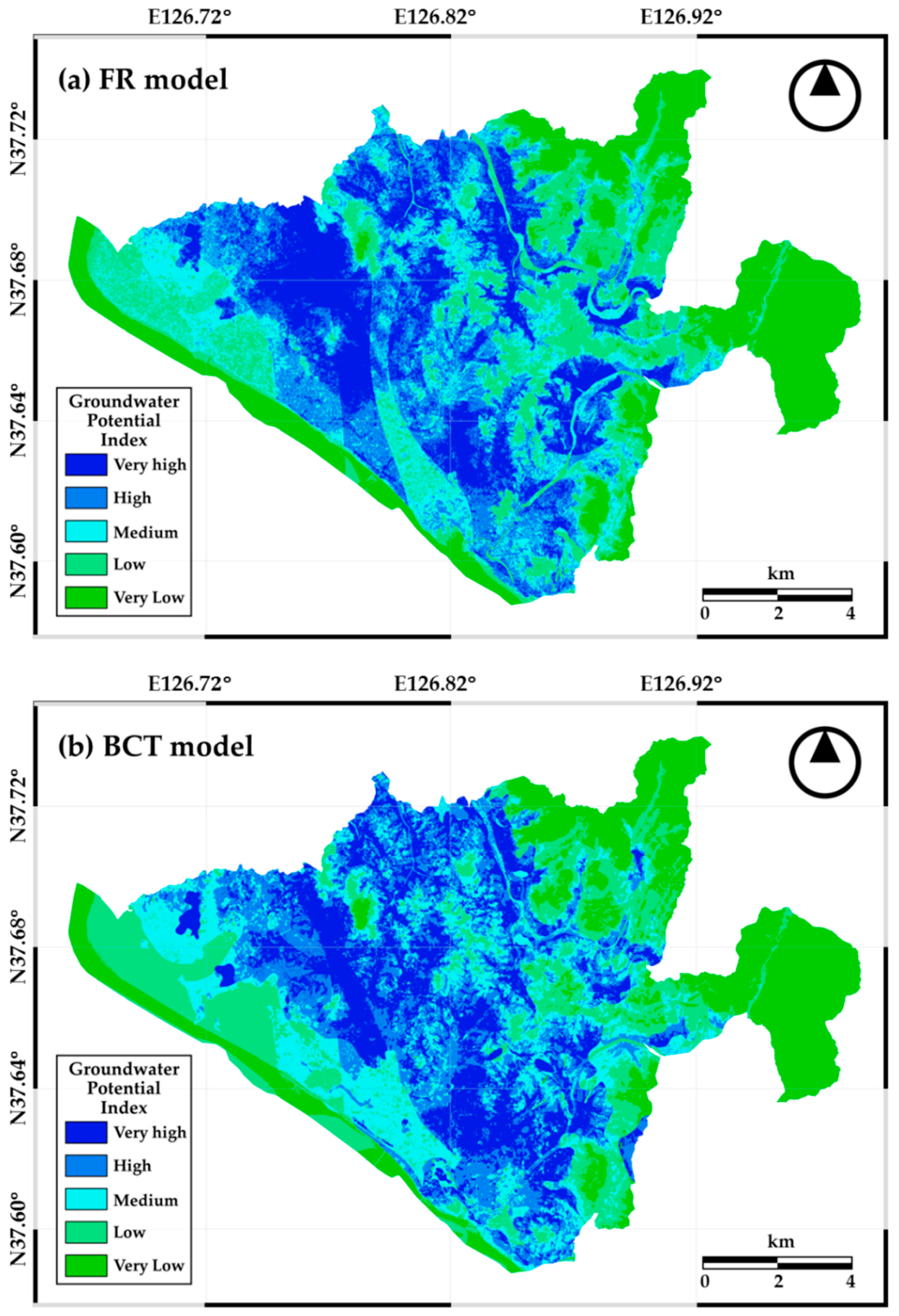
Based on the results presented in Table 3, a groundwater potential map was created by substituting and adding the FR values calculated for each class of groundwater influencing factor (Figure 6a). The groundwater potential data on maps generated through the FR model were sorted into 5 classes from very low to very high using the quantile classification technique. In terms of the areal distribution of each classification class, the very high class covered 52.72 km², accounting for 19.79% of the total area. Likewise, based on BCT results, the entire study area was classified into five groups using the quantile classification method (Figure 6b). On the BCT-derived groundwater potential map, the area with a very high potential for groundwater was 53.16 km² (19.95%), slightly larger than that on the groundwater potential map created using FR (Table 4). Also, the groundwater potential maps from both models spatially shows similar patterns with the factor of the unconsolidated aquifer. The influence of each factor can be estimated through the similarity of the spatial pattern.

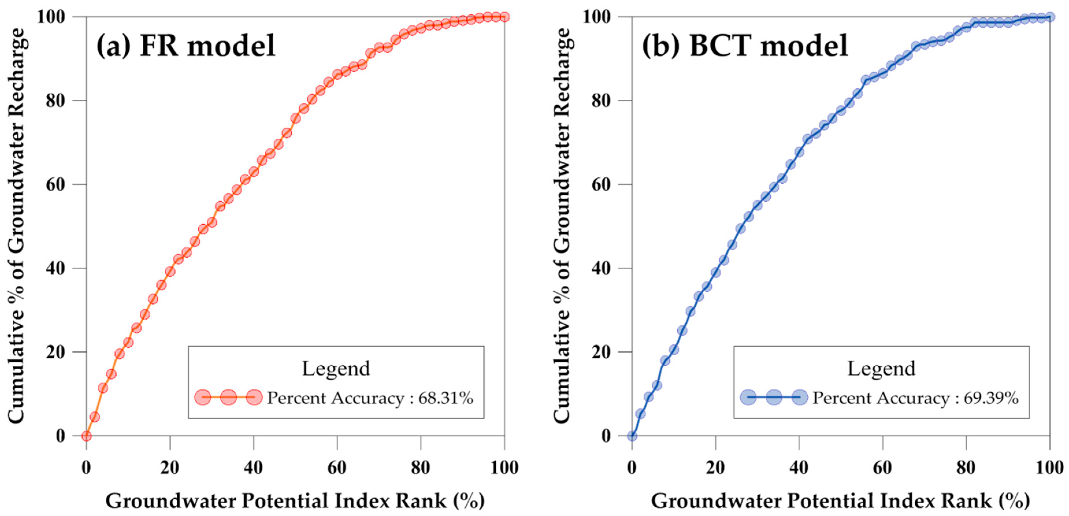
The maps resulting from groundwater potential mapping using the FR and BCT models were compared and tested using receiver operating characteristic (ROC) curves. The ROC curve is a widely used method of graphical plot that shows the capabilities of data mining models with certain thresholds [55,56]. The ROC curve is a method used to evaluate the performance of a classification model that has two categories, with a sensitivity on the x-axis and 1 − specificity on the y-axis. In this study, the categories were divided into data classes, indicating a pumping capacity above a certain level and other classes. The ROC curve method includes a success rate curve and a prediction rate curve. The success rate curve is created using the training data and indicates how well the model reflects the location of groundwater pumping capacity data used in the study. The prediction rate curve is generated using the test data and shows how well the model predicts the potential for groundwater pumping capacity [31]. The performance of the model was evaluated by calculating the area under the ROC curve (AUC), which is classified as excellent when the AUC value is 0.9–1.0, good when 0.8–0.90, and worthless when 0.7–0.8 [57]. Thus, higher values of AUC indicate a higher accuracy. The groundwater potential map prepared using FR had an accuracy of 0.6831 and that of the map prepared using the BCT model was 0.6939 (Figure 7).

5.3. Sensitivity Analysis

A sensitivity analysis was performed to assess the difference in the effect of each factor on the groundwater potential. The suitability of the test results in the previous step was assessed through the analysis. For FR and BCT models, each factor of the 13 related factors were removed from the input dataset, respectively. The degree of accuracy reduction allowed us to determine the degree of influence of each factor. As a result of the FR model, it showed about 0.46% of increase when the soil depth factor was removed from the spatial dataset (

Table 5. The predictor importance values for the boosted classification tree (BCT) analysis.

Category		Percent Accuracy of Each Model
	FR Model	Variation	BCT Model	Variation
All factors	68.31		69.39
DEM (m)	67.24	−1.07	68.69	−0.70
Slope (°)	68.24	−0.07	69.32	−0.07
Land Cover	67.99	−0.32	68.32	−1.07
Soil Drainage	68.44	0.13	69.14	−0.25
Soil Texture	68.07	−0.24	68.90	−0.49
Soil Depth	68.77	0.46	69.39	0
Timber type	68.51	0.20	69.45	0.06
Timber density	68.67	0.36	69.39	0
Geology	68.06	−0.25	69.20	−0.19
Hydrogeology	68.27	−0.04	69.39	0
Unconsolidated Aquifer	67.73	−0.58	69.12	−0.27
Fractured Rock Aquifer	68.19	−0.12	68.24	−1.15
Accumulated Precipitation	67.33	−0.98	68.86	−0.53

). Also, the test rate decreased when topographic, geology, and other factors were removed, including DEM (−1.07) accumulated precipitation (−0.98), unconsolidated aquifer (−0.58), land cover (−0.32), geology (−0.25), soil texture (−0.24), fractured rock aquifer (−0.12), slope (−0.07), and hydrogeology (−0.04); these results indicate that these factors have low influences in the FR model. For the BCT model, when the timber type factor was removed, the test rate showed a 69.45% accuracy, which is a 0.06% increase. On the other hand, there was no difference when the soil depth, timber density, and hydrogeology factors were removed. For the other factors, it showed a reduced accuracy while fractured rock aquifer and land cover showed over 1% of reduction. The sensitivity analysis showed that there was no significant change even if each input data was removed. In other words, the accuracy result of this study was considered to be the best result of applying the data mining technique in this study area.

6. Discussion and Conclusions

In this study, the groundwater potential was predicted using data mining and big data methodologies based on remote sensing data products.

A spatial database was first constructed, containing groundwater pumping capacity data and groundwater-related influencing factors. The data for each factor were produced from remote sensing products including aerial photographs and satellite images. The groundwater potential distribution for Goyang-si was generated using FR and BCT data mining models, and the results from the two models were compared. For groundwater pumping capacity data, a total of 876 data were used, of which 438 (50%) were employed as training data and 438 (50%) as test data. A total of 13 groundwater-related influencing factors were obtained and calculated from thematic maps distributed by governments and other organizations, including DEM, slope, land cover, soil drainage, soil texture, soil depth, timber type, timber density, geology, hydrogeology, unconsolidated aquifer, fractured rock aquifer, and accumulated precipitation.

An FR analysis showed how each factor correlated with the groundwater pumping capacity. The class with the strongest correlation in each factor could be used to prioritize the sites for groundwater management. In addition, the BCT model reduced the spatial uncertainty and identified the predictor importance of various factors, indicating the priority of groundwater-related factors. Therefore, through a spatial comparison of the BCT and FR results, the accuracy of groundwater potential estimation could be improved in areas with high potentials, and such areas could be managed as high priority sites.

For the BCT model, geology, timber type, timber density, DEM, and accumulated precipitation showed high predictor importance, in descending order. FR also had a strong correlation with Pinus koraiensis (2.09) in the timber type factor and was highly related to a dense forest cover. The DEM showed a possibility of high groundwater potential within approximately 10–50 m with FR values of 1.4 or higher. The accumulated precipitation showed its highest correlation at 9309–9423 mm.

Among the other factors, the FR analysis showed a high tendency of 1 or more with slopes of around 1–7 degrees in the topographical factor. In particular, DEM showed a strong relationship from 19 to 25 m, with an FR value of 1.6. For the land cover factor, the highest value was 1.44 for bare ground, providing a good indication of groundwater location characteristics. For very well-drained soil, the groundwater potential rate showed a small correlation. The groundwater potential was also correlated with increasing soil depth. The geological and hydrological influences included strong correlations with granite gneiss (2.33) and unconsolidated sediment (1.11). Unconsolidated aquifer and fractured rock aquifer had the highest correlations at 30–60 and over 120, with values of 1.42 and 1.57, respectively.

The groundwater potential map generated in this study was tested using the ROC curve and the predicted curve. The AUC value of the resulting map was around 70% for both models; the BCT model had a slightly higher accuracy rate than the FR model. The FR model is a simple and easy method for analyzing groundwater potential. Although the BCT model is more difficult to apply than the FR model, it allows the quantitative analysis of the relationships between the groundwater pumping capacity and groundwater-related influencing factors by predicting the degree of uncertainty. In addition, a sensitivity analysis was performed to show that there is little change even if each data is removed from input dataset.

The groundwater potential map created in this study could be used to survey the groundwater resources in Goyang-si in a more effective and economical way. It could also be used to establish a groundwater management plan for the sustainable use of groundwater resources. The accuracy of the groundwater potential map can be improved by examining additional factors in the study area in the future, such as hydrometeorological characteristics and groundwater usage. In addition, natural environmental data related to groundwater contamination and visualization information can be quantitatively analyzed in this geospatial data format.

Nevertheless, this study has some limitations. First, there is a lack of the groundwater level data, the amount of groundwater data, and the groundwater quality data available for research purposes. The information about the groundwater observation data in the present study area was collected from governmental organizations based on regular water quality inspection data for groundwaters included in the private groundwater survey. Ongoing research and the evaluation of the current infrastructure based on the results of groundwater potentials are essential and should be reflected in policymaking to overcome these limitations.

The relationships between the class of each groundwater-related factor and the groundwater potential should be generalized and combined in future studies. This approach could be used as a guideline to determine the thresholds for Korean groundwater management. Additionally, it is possible to collectively assess the groundwater potential in other areas in Korea, and information from this study could be used to select groundwater monitoring sites and to plan future groundwater use. With the big data methodologies, the cumulative management of groundwater pumping test data will enable groundwater potential mapping across national units with larger scale.

References

- Lytras, M.; Visvizi, A. Who uses smart city services and what to make of it: Toward interdisciplinary smart cities research. Sustainability 2018, 10, 1998. [Google Scholar] [CrossRef]
- Lytras, M.D.; Raghavan, V.; Damiani, E. Big data and data analytics research: From metaphors to value space for collective wisdom in human decision making and smart machines. Int. J. Semant. Web Inf. Syst. 2017, 13, 1–10. [Google Scholar] [CrossRef]
- Vörösmarty, C.J.; McIntyre, P.B.; Gessner, M.O.; Dudgeon, D.; Prusevich, A.; Green, P.; Glidden, S.; Bunn, S.E.; Sullivan, C.A.; Liermann, C.R.; et al. Global threats to human water security and river biodiversity. Nature 2010, 467, 555. [Google Scholar] [CrossRef] [PubMed]
- Oki, T.; Kanae, S.J. Global hydrological cycles and world water resources. Science 2006, 313, 1068–1072. [Google Scholar] [CrossRef]
- Lee, J.W.; Jung, C.G.; Kim, D.R.; Kim, S.J. Assessment of future climate change impact on groundwater level behavior in Geum river basin using SWAT. J. Korea Water Resour. Assoc. 2018, 51, 247–261. [Google Scholar]
- Korea Institute of Civil Engineering and Building Technology. Groundwater Management Basic Plan; Korea Institute of Civil Engineering and Building Technology: Gyeonggi-do, Korea, 2007. [Google Scholar]
- Graniel, C.; Morris, L.; Carrillo-Rivera, J.J. Effects of urbanization on groundwater resources of Merida, Yucatan, Mexico. Environ. Geol. 1999, 37, 303–312. [Google Scholar] [CrossRef]
- Kløve, B.; Ala-Aho, P.; Bertrand, G.; Gurdak, J.J.; Kupfersberger, H.; Kværner, J.; Muotka, T.; Mykrä, H.; Preda, E.; Rossi, P.; et al. Climate change impacts on groundwater and dependent ecosystems. J. Hydrol. 2014, 518, 250–266. [Google Scholar] [CrossRef] [Green Version]
- Bera, K.; Bandyopadhyay, J. Ground water potential mapping in Dulung watershed using remote sensing & GIS techniques, West Bengal, India. Int. J. Sci. Res. Publ. 2012, 2, 1–7. [Google Scholar]
- Lee, M.-J.; Lee, J.-H. Coupled model development between groundwater recharge quantity and climate change using GIS. J. Korean Assoc. Geogr. Inf. Stud. 2011, 14, 36–51. [Google Scholar] [CrossRef]
- Woo, N.C. Climate change and groundwater sustainability in Korea for next decade. J. Soil Groundw. Environ. 2013, 18, 1–5. [Google Scholar] [CrossRef]
- Song, S.-H.; Choi, K.-J. An appropriate utilization of agricultural water resources of Jeju island with climate change (I). J. Soil Groundw. Environ. 2012, 17, 62–70. [Google Scholar] [CrossRef]
- Mokadem, N.; Boughariou, E.; Mudarra, M.; Brahim, F.B.; Andreo, B.; Hamed, Y.; Bouri, S. Mapping potential zones for groundwater recharge and its evaluation in arid environments using a GIS approach: Case study of North Gafsa Basin (Central Tunisia). J. Afr. Earth Sci. 2018, 141, 107–117. [Google Scholar] [CrossRef]
- Nayak, P.; Rai, A.K.; Tripathy, S. Evaluating groundwater prospects using GIS techniques. Sustain. Water Resour. Manag. 2017, 3, 129–139. [Google Scholar] [CrossRef]
- Pinto, D.; Shrestha, S.; Babel, M.S.; Ninsawat, S. Delineation of groundwater potential zones in the Comoro watershed, Timor Leste using GIS, remote sensing and analytic hierarchy process (AHP) technique. Appl. Water Sci. 2017, 7, 503–519. [Google Scholar] [CrossRef]
- Şener, E.; Şener, Ş.; Davraz, A. Groundwater potential mapping by combining fuzzy-analytic hierarchy process and GIS in Beyşehir Lake Basin, Turkey. Arab. J. Geosci. 2018, 11, 1–21. [Google Scholar] [CrossRef]
- Tschritter, C.; Rawlinson, Z.; Westerhoff, R.; White, P. Aquifer classification and mapping at the national scale—Phase 1: Identification of hydrogeological units. GNS Sci. Rep. 2017, 23, 51–52. [Google Scholar]
- Mousavi, S.M.; Golkarian, A.; Naghibi, S.A.; Kalantar, B.; Pradhan, B. GIS-based groundwater spring potential mapping using data mining boosted regression tree and probabilistic frequency ratio models in Iran. AIMS Geosci. 2017, 3, 91–115. [Google Scholar]
- Sahoo, S.; Munusamy, S.B.; Dhar, A.; Kar, A.; Ram, P. Appraising the accuracy of multi-class frequency ratio and weights of evidence method for delineation of regional groundwater potential zones in canal command system. Water Resour. Manag. 2017, 31, 4399–4413. [Google Scholar] [CrossRef]
- Navane, V.S.; Sahoo, S.N. A Review of Integrated RS and GIS Technique in Groundwater Potential Zone Mapping. In Proceedings of the 22nd International Conference on Hydraulics, Water Resources and Coastal Engineering (HYDRO), Ahmedabad, Gujarat, India, 21–23 December 2017. [Google Scholar]
- Barzegar, R.; Moghaddam, A.A.; Deo, R.; Fijani, E.; Tziritis, E. Mapping groundwater contamination risk of multiple aquifers using multi-model ensemble of machine learning algorithms. Sci. Total Environ. 2018, 621, 697–712. [Google Scholar] [CrossRef]
- Golkarian, A.; Naghibi, S.A.; Kalantar, B.; Pradhan, B. Groundwater potential mapping using C5.0, random forest, and multivariate adaptive regression spline models in GIS. Environ. Monit. Assess. 2018, 190, 149. [Google Scholar] [CrossRef]
- Kordestani, M.D.; Naghibi, S.A.; Hashemi, H.; Ahmadi, K.; Kalantar, B.; Pradhan, B. Groundwater potential mapping using a novel data-mining ensemble model. Hydrogeol. J. 2018, 27, 1–14. [Google Scholar] [CrossRef]
- Luís, A.M. Development of Regional Exploration Techniques for Groundwater Resources in Semiarid Areas Through Integration of Remote Sensing and Geophysical Survey. Ph.D. Thesis, Kyoto University, Kyoto, Japan, March 2018. [Google Scholar]
- Magaia, L.A.; Goto, T.-N.; Masoud, A.A.; Koike, K. identifying groundwater potential in crystalline basement rocks using remote sensing and electromagnetic sounding techniques in Central Western Mozambique. Nat. Resour. Res. 2018, 27, 275–298. [Google Scholar] [CrossRef]
- Pradhan, B. Groundwater potential zonation for basaltic watersheds using satellite remote sensing data and GIS techniques. Open Geosci. 2009, 1, 120–129. [Google Scholar] [CrossRef] [Green Version]
- Ding, Q.; Chen, W.; Hong, H. Application of frequency ratio, weights of evidence and evidential belief function models in landslide susceptibility mapping. Geocarto Int. 2017, 32, 619–639. [Google Scholar] [CrossRef]
- Hong, H.; Chen, W.; Xu, C.; Youssef, A.M.; Pradhan, B.; Tien Bui, D. Rainfall-induced landslide susceptibility assessment at the Chongren area (China) using frequency ratio, certainty factor, and index of entropy. Geocarto Int. 2017, 32, 139–154. [Google Scholar] [CrossRef]
- Lee, S.; Lee, M.-J.; Lee, S. Spatial prediction of urban landslide susceptibility based on topographic factors using boosted trees. Environ. Earth Sci. 2018, 77, 656. [Google Scholar] [CrossRef]
- Siahkamari, S.; Haghizadeh, A.; Zeinivand, H.; Tahmasebipour, N.; Rahmati, O. Spatial prediction of flood-susceptible areas using frequency ratio and maximum entropy models. Geocarto Int. 2018, 33, 927–941. [Google Scholar] [CrossRef]
- Al-Abadi, A.M. Modeling of groundwater productivity in northeastern Wasit Governorate, Iraq using frequency ratio and Shannon’s entropy models. Appl. Water Sci. 2017, 7, 699–716. [Google Scholar] [CrossRef]
- Ke, G.; Meng, Q.; Finley, T.; Wang, T.; Chen, W.; Ma, W.; Ye, Q.; Liu, T.-Y. Lightgbm: A highly efficient gradient boosting decision tree. In Proceedings of the Advances in Neural Information Processing Systems (NIPS 2017), Long Beach, CA, USA, 4–9 December 2017; pp. 3146–3154. [Google Scholar]
- Kim, J.-C.; Lee, S.; Jung, H.-S.; Lee, S. Landslide susceptibility mapping using random forest and boosted tree models in Pyeong-Chang, Korea. Geocarto Int. 2018, 33, 1000–1015. [Google Scholar] [CrossRef]
- Lee, S.; Kim, J.-C.; Jung, H.-S.; Lee, M.J.; Lee, S. Spatial prediction of flood susceptibility using random-forest and boosted-tree models in Seoul metropolitan city, Korea. Geomat. Nat. Hazards Risk 2017, 8, 1185–1203. [Google Scholar] [CrossRef]
- Nieto, P.J.G.; García-Gonzalo, E.; Lasheras, F.S.; Fernández, J.R.A.; Muñiz, C.D.; de Cos Juez, F.J. Cyanotoxin level prediction in a reservoir using gradient boosted regression trees: A case study. Environ. Sci. Pollut. Res. 2018, 25, 1–14. [Google Scholar]
- Shin, H. Report of Research Trends Transportation Technology Evaluation Planning; Korea Institute of Construction, Ministry of Land-Transport and Maritime Affairs: Sejong City, Korea, 2008.
- Park, S.Y.; Kim, J.S. A GIS-based comparative study of frequency ratio and dempster-shafer theory for groundwater potential mapping in Busan metropolitan city. J. Korean Soc. Geosp. Inf. Sci. 2018, 26, 49–59. [Google Scholar]
- Lee, S.; Hong, S.-M.; Jung, H.-S. A support vector machine for landslide susceptibility mapping in Gangwon Province, Korea. Sustainability 2017, 9, 48. [Google Scholar] [CrossRef]
- Oh, H.-J.; Kadavi, P.R.; Lee, C.-W.; Lee, S. Evaluation of landslide susceptibility mapping by evidential belief function, logistic regression and support vector machine models. Geomat. Nat. Hazards Risk 2018, 9, 1053–1070. [Google Scholar] [CrossRef]
- Ortiz, J.A.V.; Martínez-Graña, A.M. A neural network model applied to landslide susceptibility analysis (Capitanejo, Colombia). Geomat. Nat. Hazards Risk 2018, 9, 1106–1128. [Google Scholar] [CrossRef]
- Park, S.-J.; Lee, C.-W.; Lee, S.; Lee, M.-J. Landslide susceptibility mapping and comparison using decision tree models: A Case Study of Jumunjin Area, Korea. Remote Sens. 2018, 10, 1545. [Google Scholar] [CrossRef]
- Oh, H. Landslide susceptibility analysis and validation using Weight-of-Evidence model. J. Geol. Soc. Korea 2010, 46, 157–170. [Google Scholar]
- Van Lent, J.; Hergoualc’h, K.; Verchot, L.; Oenema, O.; van Groenigen, J.W. Greenhouse gas emissions along a peat swamp forest degradation gradient in the Peruvian Amazon: soil moisture and palm roots effects. Mitig. Adapt. Strateg. Glob. Chang. 2018, 1–19. [Google Scholar] [CrossRef] [Green Version]
- Rural Development Administration. Soil Profile Description. Available online: http://soil.rda.go.kr/soil/soilact/agriCulture.jsp (accessed on 5 December 2018).
- Oh, H.-J.; Kim, Y.-S.; Choi, J.-K.; Park, E.; Lee, S. GIS mapping of regional probabilistic groundwater potential in the area of Pohang City, Korea. J. Hydrol. 2011, 399, 158–172. [Google Scholar] [CrossRef]
- Bonham-Carter, G.F. Geographic Information Systems for Geoscientists: Modelling with GIS; Elsevier: Amsterdam, The Netherlands, 2014; Volume 13. [Google Scholar]
- Razandi, Y.; Pourghasemi, H.R.; Neisani, N.S.; Rahmati, O. Application of analytical hierarchy process, frequency ratio, and certainty factor models for groundwater potential mapping using GIS. Earth Sci. Inf. 2015, 8, 867–883. [Google Scholar] [CrossRef]
- Lee, S.; Kim, Y.; Min, K. Development of spatial landslide information system and application of spatial landslide information. GIS Assoc Korea 2000, 8, 141–153. [Google Scholar]
- Freund, Y.; Schapire, R.E. Experiments with a new boosting algorithm. Proceedings of Thirteenth International Conference on International Conference on Machine Learning ICML, Bari, Italy, 3–6 July 1996; pp. 148–156. [Google Scholar]
- Friedman, J.; Hastie, T.; Tibshirani, R. The Elements of Statistical Learning; Springer: New York, NY, USA, 2001; Volume 1. [Google Scholar]
- Friedman, J.H. Stochastic gradient boosting. Comput. Stat. Data Anal. 2002, 38, 367–378. [Google Scholar] [CrossRef] [Green Version]
- Lee, S.; Hong, S.-M.; Jung, H.-S. GIS-based groundwater potential mapping using artificial neural network and support vector machine models: The case of Boryeong city in Korea. Geocarto Int. 2018, 33, 847–861. [Google Scholar] [CrossRef]
- Lee, S.; Lee, C.-W. Application of decision-tree model to groundwater productivity-potential mapping. Sustainability 2015, 7, 13416–13432. [Google Scholar] [CrossRef]
- Park, I.; Kim, Y.; Lee, S. Groundwater productivity potential mapping using evidential belief function. Groundwater 2014, 52, 201–207. [Google Scholar] [CrossRef]
- Althuwaynee, O.F.; Pradhan, B.; Lee, S. A novel integrated model for assessing landslide susceptibility mapping using CHAID and AHP pair-wise comparison. Int. J. Remote Sens. 2016, 37, 1190–1209. [Google Scholar] [CrossRef]
- Tahmassebipoor, N.; Rahmati, O.; Noormohamadi, F.; Lee, S. Spatial analysis of groundwater potential using weights-of-evidence and evidential belief function models and remote sensing. Arabian J. Geosci. 2016, 9, 79. [Google Scholar] [CrossRef]
- Zhu, W.; Zeng, N.; Wang, N. Sensitivity, specificity, accuracy, associated confidence interval and ROC analysis with practical SAS implementations. NESUG Proc. Health Care Life Sci. Baltim. Md 2010, 19, 67. [Google Scholar]
Figure 1.
The study area in this study: (a) The Korean Peninsula and (b) Goyang-si.
Figure 2.
The groundwater pumping capacity data used for training and the test.
Figure 3.
The cross-sectional data construction through digging and layering by the RDA [44].
Figure 4.
The spatial database constructed for the groundwater potential analysis: (a) DEM; (b) Slope; (c) Land cover; (d) Soil drainage;(e) Soil texture; (f) Soil depth; (g) Timber type; (h) Timber density; (i) Geology; (j) Hydrogeology; (k) Unconsolidated Aquifer; (l) Fractured Rock Aquifer and (m) Accumulated Precipitation.
Figure 5.
A flow chart outlining the study methodology.
Figure 6.
The groundwater potential maps: (a) Frequency ratio and (b) boosted classification tree.
Figure 7.
The cumulative frequency diagram showing groundwater potential index rank (x-axis) as a cumulative percentage of groundwater potential (y-axis): (a) Frequency ratio and (b) boosted classification tree.